- 1School of Mathematics, China University of Mining and Technology, Xuzhou, China
- 2School of Science, North University of China, Taiyuan, China
In this article, an
1 Introduction
Coronaviruses are a group of enveloped viruses with a positive-sense, single-stranded RNA and viral particles resembling a crown from which the name derives. They belong to the order of Nidovirales, family of Coronaviridae, and subfamily of Orthocoronavirinae. A recent coronavirus outbreak has started since December 2019. So far, the new virus has infected more than 25 million people and killed at least 842,000 of them [1–3].
In order to better study the spread and control of infectious diseases, several classical mathematical models have been discussed to understand the transmission mechanism and dynamics of the disease, such as the SI model, SIR model, SEIR model, and SEIRS model [4, 5]. Different factors are considered in different models, and the purpose of these models is finding the transmission mechanism and dynamics of the diseases for controlling the diseases. This process needs a contact between them. It is found that the best pattern of contact is contact in the networks [6–11], and study epidemic model on networks has been a hot field in mathematical biology [6–20,35].
To find the transmission mechanism, we have to know who is the infector [27]. An infector is an individual who carries the virus and can export the virus. Sometimes, an individual with the infected state may not show any symptoms of disease, and the state can be defined as asymptomatically infected. An individual with the infected state who shows symptoms of disease can be defined as symptomatically infected. Exposed state and asymptomatically infected state are more dangerous than symptomatically infected state. When a susceptible individual contacts a symptomatic one, he(she) will usually do something possible to prevent the disease spreading.
In the disease spreading process, a symptomatic infector will be restricted by individual behavior or public behavior, but a symptomatic one has a higher efficiency than an asymptomatic one. A class of works studied the role of symptomatic infectors and asymptomatic infectors in diseases infections, such as dengue virus [21, 22], malaria [23], and Norovirus [24–27]. The results of these works all show that the asymptomatic cases cannot be neglected. Recently, several mathematic models within asymptomatic infection have been studied, such as
In this article, we consider an
2 The Model
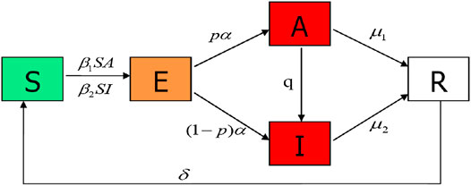
In the spread process, each node has five states: susceptible (S); exposed (E); asymptomatically infected (A), those who are infectious but have no symptoms; symptomatically infected (I), those who are infectious but have symptoms; and removed (R). The disease transmission flow is depicted in Figure 1. A susceptible individual can be infected by contact at rate
In this article, we consider an
Following [6],
For the practice, the initial condition for model (2.1) satisfies the following:
3 Dynamical Behaviors of the Model
In this section, we study the stability of disease-free equilibrium of model (2.1). First, we derive the basic reproduction number of the model.
3.1 Equilibria and Basic Reproduction Number
Lemma 3.1. Suppose that
is a positive invariant for model (2.1).The proof of this lemma is similar to that in [31]. We ignore it here. The stability analysis and numerical simulations are investigated in the positive invariant
and
In addition,
and
so,
Let
Remark 3.1.Let
Remark 3.2.If we do not consider the asymptomatic infected state, that is
Lemma 3.2.If and only if
Proof.We consider the right side of the model (2.1) to be equal to zero. Then, we obtain
Following the above equation, using
According to the condition
Substituting
and
Thus,
3.2 Stability of Disease-free and Endemic Equilibrium
Theorem 3.1.If
Proof.From the results of Lemma 3.1, Lemma 3.2, and the basic reproduction number, we only need to prove the case of
The Jacobian matrix of model (3.4) at disease-free equilibrium is given by
with
The characteristic equation of the disease-free equilibrium is
where
when
Then, we obtain
where the eigenvalues of J are all negative except zero eigenvalue when
4 Quarantine Strategies
Quarantine is helpful in controlling diseases. In this section, we will discuss three different quarantine strategies for COVID-19 disease model on networks.
4.1 Proportional Quarantine
In this case, for fixed spreading rates
Using the same method in Section 3, we obtain a self-consistency equation as follows:
By arguments similar to those in Section 3, the epidemic threshold
therefore, it can be shown that
that is,
Note that in (4.3), when
4.2 Targeted Quarantine
While proportional quarantine schemes are effective, there may be more efficient schemes due to the heterogeneous nature of scale-free networks. We introduce an upper threshold κ such that all nodes with connectivity
where
This leads to
Therefore, the epidemic threshold
Note that
If we set
which means the targeted quarantine scheme is more efficient than the uniform quarantine scheme for the same average quarantine rate.
4.3 High-Risk Quarantine
If a neighbor of a susceptible individual is infected, vaccinating this susceptible individual is called high-risk immunity [37]. We introduce the parameter σ, that is, the probability that a node is quarantined per unit time, and
This leads to
And the epidemic threshold
This means that the implementation of high-risk quarantine is effective, and the longer the period of
5 Numerical Simulations
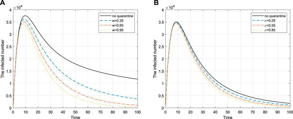
In this section, we present numerical simulations of model (2.1), (4.1) and (4.6) to illustrate the results in Section 3 and 4. Without loss of generality, we consider the dynamical process on scale-free networks with
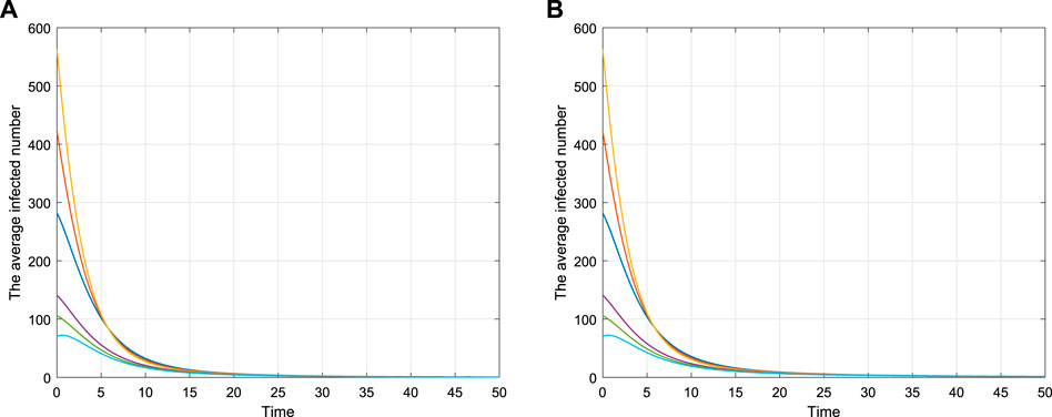
Figure 2 shows the asymptotical stability of model (2.1) with different values, and the parameter values are shown in Table 1. Figures 2A,B show the time series of the average infected number I(t) with different initial values, which is in accord with the asymptotical stability of the disease-free equilibrium.

TABLE 1. Parameters of Figure 2

TABLE 2. Parameters of Figure 4
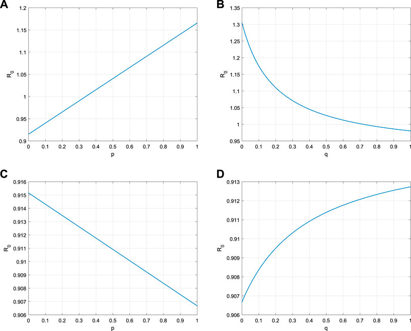
The sensitivity analysis of the basic reproduction number R0 can be performed by model parameters. It is easy to obtain that
Equation (5.1) shows
6 Conclusion and Discussion
In this article, we have generalized a traditional homogeneous epidemic model with asymptomatic infectors to a network case to study the spread of COVID-19. As one can see, homogeneous epidemic models can be considered as a special case of network epidemic models, and network epidemic models are more realistic and refined description of disease propagation in population. Considering two cases of infected state (show symptoms and show no symptoms), we investigated an
The SEAIRS model is an extension of the SEAIRS model, and it is a case of the
At the same time, we have also discussed proportional, targeted quarantine and high-risk quarantine schemes for network models. The result of Leung et al. [27] by illustration is suitable for Norovirus and measles. Different from their work, the formulaic result seems to be unsuitable for any kind of disease, for none of the parameters in the model is assigned to a specific value. In fact, for different disease, the parameters in the model may present special values. COVID-19 is now spreading faster abroad. Susceptible people will also be infected by asymptomatic patients. If not controlled, the epidemic will spread more widely and the number of infected people will be more difficult to control. The epidemic situation in China was obviously well controlled after the implementation of the strategy of lockdown, and other quarantine strategies. Therefore, the model and quarantine strategy in this article can also be applied to other countries. And, we hope that the results will be helpful to study and control the spread of COVID-19 disease.
Data Availability Statement
The original contributions presented in the study are included in the article/Supplementary Material; further inquiries can be directed to the corresponding author.
Author Contributions
ML and YS designed the study, and WL and ML carried out the analysis and contributed to writing the article. XF and YS performed numerical simulations.
Funding
Research Project Supported by Fund for Shanxi 1331KIRT and the outstanding youth fund of North University of China.
Conflict of Interest
The authors declare that the research was conducted in the absence of any commercial or financial relationships that could be construed as a potential conflict of interest.
References
1.Report on novel coronavirus pneumonia epidemic in real time. (2020) https://voice.baidu.com/act/newpneumonia/newpneumonia/.
2. Tang B, Wang X, Li Q, Bragazzi NL, Tang SY, Xiao YN, et al. Estimation of the transmission risk of the 2019-nCoV and its implication for public health interventions. J Comput Math (2020) 9:462. doi:10.3390/jcm9020462
3. Tang B, Bragazzi NL, Li Q, Tang S, Xiao Y, Wu J. An updated estimation of the risk of transmission of the novel coronavirus (2019-nCov). Infect Dis Model (2020) 5:248–55. doi:10.1016/j.idm.2020.02.001
5. Li MY, Muldowney JS, van den Driessche P. Global stability of SEIRS models in epidemiology. Can Appl Math Q (1999) 7:409–25.
6. Pastor-Satorras R, Vespignani A. Epidemic spreading in scale-free networks. Phys Rev Lett (2001) 86:3200–3. doi:10.1103/PhysRevLett.86.3200
7. Butts CT. Revisiting the foundations of network analysis. Science (2009) 325(5939):414–6. doi:10.1126/science.1171022
9. Vespignani A. Predicting the behavior of techno-social systems. Science (2009) 325(5939):425–8. doi:10.1126/science.1171990
10. Vespignani A. Modeling dynamical processes in complex socio-technical systems. Nat Phys (2012) 8:32–9. doi:10.1038/nphys2160
11. Pastor-Satorras R, Castellano C, Van Mieghem P, Vespignani A. Epidemic processes in complex networks. Rev Mod Phys (2015) 87:925–79. doi:10.1017/cbo9780511791383.010
12. Wang B, Han Y, Tanaka G. Interplay between epidemic spread and information propagation on metapopulation networks. J Theor Biol (2017) 420:18–25. doi:10.1016/j.jtbi.2017.02.020
13. Liu G, Liu Z, Jin Z. Dynamics analysis of epidemic and information spreading in overlay networks. J Theor Biol (2018) 444:28–37. doi:10.1016/j.jtbi.2018.02.010
14. Zhang X, Shan C, Jin Z, Zhu H. Complex dynamics of epidemic models on adaptive networks. J Differ Equ (2019) 266(1):803–32. doi:10.1016/j.jde.2018.07.054
15. Massad E, Ma S, Chen M, Struchiner C, Stollenwerk N, Mara A. Scale-free network of a dengue epidemic. Appl Math Comput (2008) 195:376–81. doi:10.1016/j.amc.2007.04.102
16. Mishra BK, Pandey SK. Dynamic model of worms with vertical transmission in computer network. Appl Math Comput (2011) 217:8438–46. doi:10.1016/j.amc.2011.03.041
17. Zhang JP, Jin Z. The analysis of an epidemic model on networks. Appl Math Comput (2011) 217:7053–64. doi:10.1007/978-3-662-47824-0_3
18. Nian F, Yao S. The epidemic spreading on the multi-relationships network. Appl Math Comput (2018) 339:866–73. doi:10.1016/j.amc.2018.07.030
19. Wang ZS, Guo QT, Sun SW, Xia CY. The impact of awareness diffusion on SIR-like epidemics in multiplex networks. Appl Math Comput (2019) 349:134–47. doi:10.1016/j.chaos.2019.109425
20. Wang ZS, Xia CY, Chen ZQ, Chen GR. Epidemic propagation with positive and negative preventive information in multiplex networks. IEEE Trans Cybern (2020) doi:10.1109/TCYB.2019.2960605
21. Grunnill M. An exploration of the role of asymptomatic infections in the epidemiology of dengue viruses through susceptible, asymptomatic, infected and recovered (SAIR) models. J Theor Biol (2018) 439:195–204. doi:10.1016/j.jtbi.2017.12.009
22. Mishra A, Gakkhar S. Modeling of Dengue with impact of asymptomatic infection and ADE factor. Differ Equ Dyn Syst (2018) 19:1–17. doi:10.1007/s12591-018-0436-4
23. Beretta E, Capasso V, Garao DG. A mathematical model for malaria transmission with asymptomatic carriers and two age groups in the human population. Math Biosci (2018) 300:87–101. doi:10.1016/j.mbs.2018.03.024
24. Gallimore CI, Cubitt D, du Plessis N, Gray JJ. Asymptomatic and symptomatic excretion of noroviruses during a hospital outbreak of gastroenteritis. J Clin Microbiol (2004) 42:2271–4. doi:10.1128/jcm.42.5.2271-2274.2004
25. García C, DuPont HL, Long KZ, Santos JI, Ko G. Asymptomatic norovirus infection in Mexican children. J Clin Microbiol (2006) 44:2997–3000. doi:10.1128/JCM.00065-06
26. Bucardo F, Nordgren J, Carlsson B, Kindberg E, Paniagua M, Möllby R, et al. Svensson L. Asymptomatic norovirus infections in Nicaraguan children and its association with viral properties and histo-blood group antigens. Pediatr Infect Dis J (2010) 29:934–9. doi:10.1097/INF.0b013e3181ed9f2f
27. Leung KY, Trapman P, Britton T. Who is the infector? Epidemic models with symptomatic and asymptomatic cases. Math Biosci (2018) 301:190–8. doi:10.1016/j.mbs.2018.04.002
28. Chisholm RH, Campbell PT, Wu Y, Tong SYC, McVernon J, Geard N Implications of asymptomatic carriers for infectious disease transmission and control. R Soc Open Sci (2018) 5:172341. doi:10.1098/rsos.172341
29. De la Sen M, Alonso-Quesada S, Ibeas A, Nistal R. On an SEIADR epidemic model with vaccination, treatment and dead-infectious copses removal controls. Math Comput Simul (2019) 163:47–79. doi:10.3390/ijerph16152689
30. Ma Y, Liu M, Hou Q, Zhao J. Modelling seasonal HFMD with the recessive infection in Shandong, China. Math Biosci Eng (2013) 10:1159–71. doi:10.3934/mbe.2013.10.1159
31. Cao J, Wang Y, Alofi A, Mazrooei AA, Elaiw A. Global stability of an epidemic model with carrier state in heterogeneous networks. IMA J Appl Math (2015) 80:1025. doi:10.1093/imamat/hxu040
32. van den Driessche P, Watmough J. Reproduction numbers and sub-threshold endemic equilibria for compartmental models of disease transmission. Math Biosci (2002) 180:29–48. doi:10.1016/s0025-5564(02)00108-6
33. Liu J, Zhang T. Epidemic spreading of an SEIRS model in scale-free networks. Commun Nonlinear Sci Numer Simulat (2011) 16:3375–84. doi:10.1063/1.5001176
34. Zhao XQ, Jing ZJ. Global asymptotic behavior in some cooperative systems of functional differential equations. Can Appl Math Q (1996) 4:421–44.
35. Barthélemy M, Barrat A, Pastor-Satorras R, Vespignani A. Velocity and hierarchical spread of epidemic outbreaks in scale-free networks. Phys Rev Lett (2004) 92:178701. doi:10.1103/PhysRevLett.92.178701
36. Yorke JA, London WP. Recurrent outbreaks of measles, chickenpox and mumps. II. Systematic differences in contact rates and stochastic effects. Am J Epidemiol (1973) 98:469–82. doi:10.1093/oxfordjournals.aje.a121575
Keywords: COVID-19 epidemic, networks, asymptomatic, the basic reproduction number, quarantine
Citation: Li W, Fu X, Sun Y and Liu M (2021) Dynamical Analysis of a Mathematical Model of COVID-19 Spreading on Networks. Front. Phys. 8:601459. doi: 10.3389/fphy.2020.601459
Received: 01 September 2020; Accepted: 25 November 2020;
Published: 18 January 2021.
Edited by:
Chengyi Xia, Tianjin University of Technology, ChinaReviewed by:
Chuansheng Shen, Anqing Normal University, ChinaWeigang Sun, Hangzhou Dianzi University, China
Copyright © 2021 Li, Fu, Sun and Liu. This is an open-access article distributed under the terms of the Creative Commons Attribution License (CC BY). The use, distribution or reproduction in other forums is permitted, provided the original author(s) and the copyright owner(s) are credited and that the original publication in this journal is cited, in accordance with accepted academic practice. No use, distribution or reproduction is permitted which does not comply with these terms.
*Correspondence: Maoxing Liu, bGl1bWFveGluZ0AxMjYuY29t
 Wang Li1
 Xinjie Fu
 Maoxing Liu


