Confined Brownian Motion Tracked With Motion Blur: Estimating Diffusion Coefficient and Size of Confining Space

Mesoscopic environments and particles diffusing in them are often studied by tracking such particles individually while their Brownian motion explores their environment. Environments may be, e.g., a domain in a cell membrane, an interior compartment of a cell, or an engineered nanopit. Particle trajectories are typically determined from time-lapse recorded movies. These are recorded with sufficient exposure time per frame to be able to detect and localize particles in each frame. Since particles move during this exposure time, particles image with motion blur. This motion blur can compromise estimates of diffusion coefficients and the size of the confining domain if not accounted for correctly. We do that here. We give explicit and exact expressions for the variance of measured positions and the mean-squared displacement of a Brownian particle confined in, respectively, a 1D box, a 2D box, a 2D circular disc, and a 3D sphere. Our expressions are valid for all exposure times, irrespective of the size of the confining space and the value of the diffusion coefficient. They apply also in the common case where the exposure time is smaller than the time-lapse due, e.g., to “dead time” caused by the readout process in the camera. These expressions permit determination of diffusion coefficients and domain sizes for given movies for the simple geometries we consider. More important, the trends observed in our exact results when parameter values are varied are valid also for more complex geometries for which no exact analytical solutions exist. Wherever the underlying physics is the same, the exact quantitative description of its consequences provided here is portable as a qualitative and semi-quantitative understanding of its consequences in general. The results may also be useful for other types of reflected Brownian motion than those occurring in single-particle tracking, e.g., in nuclear magnetic resonance imaging techniques. For use in that particular context, we briefly discuss the effects of confinement on anisotropic Brownian motion imaged with motion blur.

1 Introduction

In many branches of science, individual particles or molecules are labeled fluorescently in order to track and characterize their motion. To this end, they must be sufficiently isolated from each other in time and/or space, e.g., by sparse labeling [1] or super-resolution microscopies [2]. Only then may their centers be found with a precision that increases with the number of photons recorded [3]. When it does, nanometer precision is obtained routinely. In this manner, single-particle tracking is used extensively to uncover, e.g., the organization and dynamics of biology at its shortest length scale [4] and its interactions with nanoparticles [5]. One key advantage of single-particle tracking is that, with sufficiently long trajectories, it yields single-particle results. With sample-averaging unnecessary, it can detect heterogeneity in a population. Moreover, if such heterogeneity is absent, it can detect anomalous behavior in individual particles. Thus spotted before averaging, such outliers can be excluded from samples before sample-averages are calculated. This can improve accuracy and precision of estimates substantially.

Since the molecules and particles are studied under ambient conditions, they undergo Brownian motion. Various methods of various qualities are used to estimate diffusion coefficients from recorded particle trajectories describing free Brownian motion [6, 7]. Here, we address how to do similar estimates for Brownian motion in confined spaces: for example, a domain in a cell membrane, a compartment inside a cell, or an engineered nanopit [4, 8–10]. Such motion in confined domains and the properties of the domains themselves are important. Indeed, nano-domains in cell membranes, such as lipid nano-domains and nano-domains created by cellular filaments, are involved in multiple biological mechanisms, such as signal processing, membrane trafficking, and various diseases [11–13]. Moreover, single-particle tracking of nano-particles is often used to characterize lab-on-a-chip devices and thus the importance of single-particle tracking for characterization of particles and their confining environments.

The implementation of single-particle tracking may, however, itself confound results obtained with it. In order to track a fluorescently labeled particle or molecule, one records a time-lapse movie of micrographs of the particle. Typically, the dim signal from its fluorescent label is recorded with a highly sensitive camera. Each frame of the time-lapse movie must have recorded enough photons from the label to permit detection and localization of the particle in that frame [14]. So, a sufficiently long exposure time is used. The particle, however, moves during exposure. Since typical exposure times last tens of milliseconds, they are much longer than the characteristic time-scale of the particle's inertial motion. The particle thus undergoes Brownian motion while being imaged. This creates motion blur, and the observed position essentially is the time-average over positions visited by the particle during exposure. This has consequences for the statistics of motion, such as variances of measured positions of the particle and its mean-squared displacement (MSD).

While the effects of motion blur on the statistics of free Brownian motion have been studied in detail [6, 14–16], less effort has been devoted to its effects in the case of confined Brownian motion. Clearly, if the exposure time is very long, the particle visits all of a confining domain many times during a single exposure time. Thus, if the domain is smaller than the diffraction limit, super-localization techniques will locate the particle at the centroid of the confining domain if at all. Such consequences of motion blur have been observed [17], and approximate formulas that correct for these effects have been developed for specific geometries [18]. Their quality, unfortunately, depends on the values of experimental parameters. Therefore, we here derive exact expressions for the variances of positions and the MSD for Brownian particles in confinement recorded with motion blur. Specifically, we treat the cases of 1D Brownian motion confined to a box, 2D Brownian motion confined, respectively, to a box and to a circular disc, and 3D Brownian motion confined to a sphere. Our formulas are valid for all frame rates, irrespective of the value of the diffusion coefficient and the size of the confining domain. We also model the common case of “dead time” making the exposure time shorter than the inverse frame rate. While our exact results are derived for uniform and isotropic Brownian motion, we also discuss the implications of confinement and motion blur on anisotropic Brownian motion confined to a 2D disc. We do this using simulated trajectories. We compare the statistics obtained from those trajectories to the theory for the isotropic case.

We note that confined (sometimes called reflected) Brownian motion also plays an important role in other research fields, e.g., in probability theory and nuclear magnetic resonance (NMR) imaging. Time-averaging also may influence results there, e.g., in pulsed field-gradient spin-echo NMR, where the diffusion of the spins during the finite duration of the pulse causes that the pores in materials appear smaller than they are (for a review, see [19, Sec. II.B]).

2 Results

2.1 True Positions Versus Measured Positions

In order to track a fluorescently labeled particle in a fluorescence microscopy experiment, one records a movie of it. Typically, one uses a constant time-lapse, $\text{Δ}t$, between frames.¹ If a particle's true position was $x_0$ at time $t_0$, we let $x\left(t|x_0,t_0\right)$ denote its true position at time t. If positions could be recorded instantaneously, we could sample positions $x_j=x\left(t_j|x_0,t_0\right)$ at equidistant discrete points in time, $t_j=j\text{Δ}t$. That is, however, not how positions are recorded in camera-based single-particle tracking. Instead, $\text{Δ}t$ is typically divided into two complementary parts, $\text{Δ}{t}_{\text{open}}$ and $\text{Δ}{t}_{\text{closed}}$. Thus, $\text{Δ}t=\text{Δ}{t}_{\text{open}}+\text{Δ}{t}_{\text{closed}}$. The camera shutter is open during a finite exposure time, $\text{Δ}{t}_{\text{open}}$, in order to record a sufficient number of photons to determine the particle's position with the desired precision [3]. The time interval $\text{Δ}{t}_{\text{closed}}$ may be a necessary “dead time” between frames due to finite duration of readout processes in the camera. In general, $\text{Δ}{t}_{\text{open}}\le \text{Δ}t$, and equality is achieved only if the camera shutter is left open during the entire time-lapse.

Finite exposure time can be accounted for by introducing the shutter function $s_j\left(t\right)$, a non-negative function that integrates to unity over the time interval $\text{Δ}t$ [15]. For the present case, the shutter function is a step function with $s_j\left(t\right)=1/\text{Δ}{t}_{\text{open}}$ for $t\in [t_j-\text{Δ}{t}_{\text{open}},t_j]$ and 0 otherwise. More advanced shutter functions can be considered [15], but they are less relevant in practice.

Since the particle moves during the recording of its position, its measured position is affected by motion blur. That position, $x_{\text{msr}}\left(t_j|x_{j-1},t_{j-1}\right)$, is found as

$x_{\text{msr},\text{j}}\equiv x_{\text{msr}}\left(t_j|x_{j-1},t_{j-1}\right)={{{\displaystyle \int }}^{\text{}}}_{t_{j-1}}^{t_j}{s}_j\left(t\right)x\left(t|x_{j-1},t_{j-1}\right)dt=\frac{1}{\text{Δ}{t}_{\text{open}}}{{{\displaystyle \int }}^{\text{}}}_{t_j-\text{Δ}{t}_{\text{open}}}^{t_j}x\left(t|x_{j-1},t_{j-1}\right)dt,(1)$

provided that it started at position $x_{j-1}$ at $t_{j-1}$ and that the estimated position is the temporal average over the positions in the trajectory of the particle, $x\left(t|x_{j-1},t_{j-1}\right)$, during the exposure time $\text{Δ}{t}_{\text{open}}$. The difference between the true positions, $x_j$, and the measured positions, $x_{\text{msr}}\left(t_j\right)$, is illustrated in Figure 1A for free diffusion.

FIGURE 1

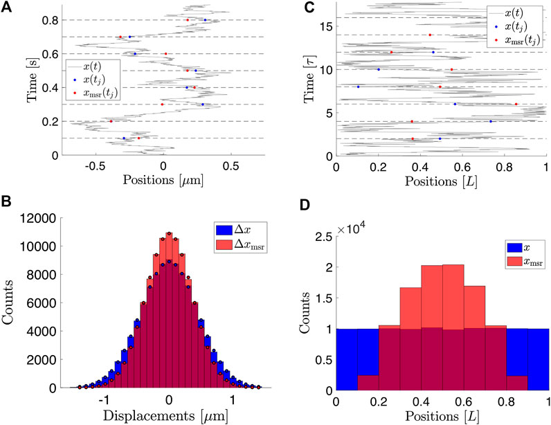
FIGURE 1. Consequences of finite exposure time for the measured positions of a Brownian particle. (A) Simulated positions of a free Brownian particle with $D=1{\left(\mu \text{m}\right)}^2/\text{s}$, $\text{Δ}t=\text{Δ}{t}_{\text{open}}=0.1$ s. In a time-lapse movie of it, in the (artificial) case of instantaneous recording of positions, the particle’s positions $x_j$ are its true positions measured at the end of each time interval, i.e., at times $t_j=j\text{Δ}t$ (blue dots). In the (realistic) case of finite exposure time, the measured positions $x_{\text{msr}}\left(t_j\right)$ are the time-averaged positions visited by the particle during the exposure time, as defined in Eq. 1 (red dots). (B) Histograms of the displacements of the true, $\text{Δ}{x}_j=x_j-x_{j-1}$, and the measured, $\text{Δ}{x}_{\text{msr}}\left(t_j\right)=x_{\text{msr}}\left(t_j\right)-x_{\text{msr}}\left(t_{j-1}\right)$, positions. Note that the variance of the measured displacements is smaller than the variance of the true displacements: motion blur effectively low-pass filters the true trajectory, which suppresses rapid displacements, so large displacements are less likely to occur within a time-lapse in the blurred trajectory. (C) Same as (A) for a particle diffusing in a 1D box at $[0,L]$ with $\tau =L^2/\left(4D\right)$ and $\text{Δ}t=\text{Δ}{t}_{\text{open}}=2\tau$. (D) Histograms of the positions (not the displacements) obtained as in C. Note that while the true position visits all positions in the box with equal probability, the finite exposure time reduces the variance of the measured positions such that the confining domain appears smaller than it is.

Below, we explore the consequences of this time-averaging on the variance and the mean-squared displacement (MSD) for Brownian motion in confining spaces. For free Brownian motion, these effects are discussed at length in, e.g., [6, 14, 15].

In real measurements, the measured position of a particle also contains a localization error due to photon shot noise. In practice, localization errors may be important in the analysis of experimental data, but we present our formulas without localization errors to keep them simple. In Section 4.5, we briefly describe how to account also for localization errors.

2.2 Free Brownian Motion

We consider a particle embedded in a fluid at rest at finite temperature, subject only to the fluctuating thermal forces from the fluid surrounding it. We assume that the time-lapse $\text{Δ}t$, with which the particle is observed, is long relatively to the inertial time-scale of the particle’s thermal motion. Then, Einstein’s original description of free Brownian motion applies. In this case, the time-dependence of the probability density P to find the Brownian particle at position x at time t, given that it was at position $x_0$ at time $t_0$, is governed by Fick’s second law of diffusion (1855), the Fokker–Planck equation [20],

$\frac{\partial P\left(x,t|x_0,t_0\right)}{\partial t}=D\frac{{\partial }^{2}P\left(x,t|x_0,t_0\right)}{\partial x^2},(2)$

with the initial condition $P\left(x,t_0|x_0,t_0\right)=\delta \left(x-x_0\right)$. Here, D is the diffusion constant.

With the boundary conditions $P\left(x,t|x_0,t_0\right)\to 0$ for $x\to \pm \infty$, for all $t>t_0$ (= closed boundaries at $x=\pm \infty$), the solution to Eq. 2 is

$P_{\text{free}}\left(x,t|x_0,t_0\right)=\frac{1}{\sqrt{4\pi D\left(t-t_0\right)}}\text{exp}\left[-\frac{{\left(x-x_0\right)}^2}{4D\left(t-t_0\right)}\right].(3)$

That is, the conditional probability density is normal with mean $x_0$ and variance ${\sigma }^2=2D\left(t-t_0\right)$.

2.2.1 Statistics of Displacements for Instantaneously Sampled Positions

As a consequence, consecutive sampled positions of a Brownian particle are related by displacements $\text{Δ}{x}_j\equiv x_j-x_{j-1}$ that are normally distributed with mean and covariance,

$\langle \text{Δ}{x}_j\rangle =0\text{ for all }j,(4)$

$\langle {\left(\text{Δ}{x}_j\right)}^2\rangle =2D\text{Δ}t\text{ for all }j,(5)$

$\langle \text{Δ}{x}_j\text{Δ}{x}_k\rangle =0\text{ for }j\ne k.(6)$

An example of time-lapse sampled positions of a Brownian particle is shown in Figure 1A.

Equation 2 also gives the mean-squared displacement,

$\text{MSD}\left(n\right)=\langle {\left(x_{j+n}-x_j\right)}^2\rangle =2Dn\text{Δ}t,(7)$

with its signature proportionality to the time lag $n\text{Δ}t$ with constant of proportionality $2D$. This property is often used to estimate the diffusion coefficient from trajectory data. To this end, $2D$ is determined as the slope in a fit of a straight line to the MSD estimated from data. This and other methods for determination of D are still discussed in the literature [7, 21], but for trajectories with signal-to-noise ration SNR $=\sqrt{D\text{Δ}t}/{\sigma }_{\text{loc}}>1$, D is certainly determined optimally by comparing the sample variance of the particle’s positions with Eq. 5 [6, 7].

2.2.2 Motion Blur Reduces Variances of Displacements and Correlates Them

Since motion blur effectively acts as a low-pass filter, the statistical properties of displacements $\text{Δ}{x}_{\text{msr},j}=x_{\text{msr},j}-x_{\text{msr},j-1}$ for measured positions are different from those of the true positions $\text{Δ}{x}_j=x_j-x_{j-1}$. For the shutter function $s_j\left(t\right)$ introduced above, the displacements of the measured positions have the properties [6, 7, 15]

$\langle {\left(\text{Δ}{x}_{\text{msr},j}\right)}^2\rangle =2D\text{Δ}t\left(1-\frac{\text{Δ}{t}_{\text{open}}}{3\text{Δ}t}\right),(8)$

$\langle \text{Δ}{x}_{\text{msr},j}\text{Δ}{x}_{\text{msr},j+1}\rangle =D\text{Δ}{t}_{\text{open}}/3,(9)$

$\langle \text{Δ}{x}_{\text{msr},j}\text{Δ}{x}_{\text{msr},\ell }\rangle =0\text{ for }|j-\ell |>1.(10)$

So, the motion blur reduces the variance of the displacements and introduces a nearest-neighbor correlation between them. Both effects are proportional to $\text{Δ}{t}_{\text{open}}$. The variance decreases from its maximal value, $2D\text{Δ}t$, at $\text{Δ}{t}_{\text{open}}=0$ to its minimum, $4D\text{Δ}t/3$, at $\text{Δ}{t}_{\text{open}}=\text{Δ}t$, see Figure 1B. Consequently, the value for D is underestimated even in the absence of localization errors if motion blur is present in measurements due to finite exposure time but is ignored, and the sample variance of the displacements of the measured positions is used as a naive estimate of the diffusion coefficient D.

The MSD of the measured positions for $n\ge 1$, however, is still linear in the time lag $n\text{Δ}t$ with slope $2D$, though offset by a constant due to the motion blur,

$\text{MSD}\left(n\right)=\langle {\left(x_{\text{msr},j+\text{n}}-x_{\text{msr},j}\right)}^2\rangle =2Dn\text{Δ}t-2D\text{Δ}{t}_{\text{open}}/3.(11)$

Consequently, a fit of a straight line to the MSD estimated from positions subject to motion blur will return the true value of D on average. However, unless data are very rich, superior alternatives for the determination of D exist also for this case [6, 7].

2.3 Brownian Motion in 1D Confinement

To account for the statistical effects of confinement, we first consider the simplest possible case, a particle diffusing in 1D in a box of length L. Let x denote the coordinate of the particle with axis chosen such that the box has $x\in [0,L]$. Equation 2 holds also in this box, but with closed boundary conditions, i.e.,

${\frac{\partial P\left(x,t|x_0,t_0\right)}{\partial x}|}_{x=0,L}=0\text{ for all }t>t_0.(12)$

For initial condition $P\left(x,t_0|x_0,t_0\right)=\delta \left(x-x_0\right)$ with $0<x_0<L$, $P\left(x,t|x_0,t_0\right)$ is found by separation of variables [22] and is

$P\left(x,t|x_0,t_0\right)=\frac{1}{L}+\frac{2}{L}{\displaystyle \sum }_{n=1}^{\infty }\text{exp}\left[-{\left(\frac{n\pi }{2}\right)}^2\frac{t-t_0}{\tau }\right]\text{cos}\left(\frac{n\pi x}{L}\right)\text{cos}\left(\frac{n\pi x_0}{L}\right).(13)$

Here, we have introduced the characteristic time-scale $\tau \equiv {\left(L/2\right)}^2/D$. Below, we use Eq. 13 to calculate an exact expression for the variance and the MSD for positions measured using finite exposure time.

Brownian motion confined to a 2D square or rectangular box is described by the independent motion of each of two Cartesian coordinates in their respective 1D boxes.

2.3.1 Variance of Positions Recorded With Motion Blur for a Brownian Particle in a 1D Box

In the limiting case of instantaneous recording of exact positions, there is uniform probability density $1/L$ to observe the particle anywhere in the 1D box (Figures 1D, 2A). Consequently, the variance of the particle’s position is $\text{var}\left(x_{\text{msr}}\right)=L^2/12$. However, for $\text{Δ}{t}_{\text{open}}/\tau$ non-negligible, the distribution of measured particle positions depends on the value of $\text{Δ}{t}_{\text{open}}/\tau$ (Figures 2B,C). This is because motion-blurred positions are averages over consecutive true positions, and it is unlikely that all contributions to such an average are close to a boundary when $\text{Δ}{t}_{\text{open}}/\tau$ is non-negligible. As a result, the confining domain appears smaller than it is [17]. On the other hand, if $\text{Δ}{t}_{\text{open}}/\tau \gg 1$, the particle visits most of the confining domain during each exposure and all measured positions thus appear in the center of the box with a vanishing positional variance, $\text{var}\left(x_{\text{msr}}\right)\simeq 0$, as consequence.

FIGURE 2

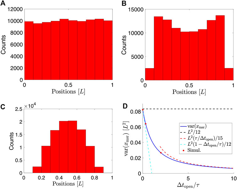
FIGURE 2. Histograms of measured positions for $\text{Δ}{t}_{\text{open}}/\tau$ = 0.01 (A), 0.33 (B), and 2 (C) for simulated Brownian motion of a particle in a 1D box. (D) The variance of measured positions $\text{Δ}{t}_{\text{open}}/\tau$ for the exact expression in Eq. 18 (blue full line), the approximate expression in Eq. 19 valid for $\text{Δ}{t}_{\text{open}}/\tau \gg 1$ (red dashed line), and the approximate expression in Eq. 20 valid for $\text{Δ}{t}_{\text{open}}/\tau \ll 1$ (cyan dashed line). Horizontal black dashed line: variance = $L^2/12$, the value for $\text{Δ}{t}_{\text{open}}/\tau \to 0$. Red dots: the sample variances of the simulated data in (A)–(C).

In practice, $\text{Δ}{t}_{\text{open}}/\tau$ is non-negligible. In order to obtain expressions for, respectively, the variance and the MSD for a particle in confinement including the effect of motion blur, valid for all values of $\text{Δ}{t}_{\text{open}}/\tau$, we follow Wong and Halvorsen [23], who used a similar calculation for a particle in a harmonic potential. In the process, we also account for the possibility that $\text{Δ}{t}_{\text{open}}<\text{Δ}t$.

The variance of the measured positions is

$\text{var}\left(x_{\text{msr}}\right)\equiv \langle x_{\text{msr}}^2\rangle -{\langle x_{\text{msr}}\rangle }^2=\langle x_{\text{msr}}^2\rangle -\frac{L^2}{4},(14)$

where the average $\langle \cdot \rangle$ is over all possible trajectories. Here, $\langle x_{\text{msr}}\rangle =L/2$, due to symmetry. Assuming a uniform distribution of initial positions, i.e., $p\left(x_0\right)=1/L$ for $0<x_0<L$ and zero otherwise, the variance is

$\text{var}\left(x_{\text{msr}}\right)={{\displaystyle \int }}^{\text{}}d{x}_{0}p\left(x_0\right){\langle x_{\text{msr}}{\left(x_0\right)}^2\rangle }_0-\frac{L^2}{4}=\frac{1}{L}{{\displaystyle \int }}^{\text{}}d{x}_0{\langle x_{\text{msr}}{\left(x_0\right)}^2\rangle }_0-\frac{L^2}{4},(15)$

where ${\langle \cdot \rangle }_0$ means averaging over all trajectories starting at the position $x_0$. We then insert $x_{\text{msr}}\left(t|x_0\right)$ from Eq. 1 and write

$\begin{array}{c}{\langle x_{\text{msr}}{\left(x_0\right)}^2\rangle }_0={\langle {{{\displaystyle \int }}^{\text{}}}_0^{\text{Δ}t}dt{{{\displaystyle \int }}^{\text{}}}_0^{\text{Δ}t}d{t}^{\prime }{s}_1\left(t^{\prime }\right)s_1\left(t\right)x\left(t^{\prime }|x_0\right)x\left(t|x_0\right)\rangle }_0\\ =\frac{2}{{\left(\text{Δ}{t}_{\text{open}}\right)}^2}{{{\displaystyle \int }}^{\text{}}}_{\text{Δ}t-\text{Δ}{t}_{\text{open}}}^{\text{Δ}t}d{t}^{\prime }{{{\displaystyle \int }}^{\text{}}}_{\text{Δ}t-\text{Δ}{t}_{\text{open}}}^{t^{\prime }}dt{\langle x\left(t^{\prime }|x_0\right)x\left(t|x_0\right)\rangle }_{0,t^{\prime }>t}.\end{array}(16)$

The time-ordered auto-correlation function can be expressed via the conditional probability density in Eq. 13,

${\langle x\left(t|x_0\right)x\left(t^{\prime }|x_0\right)\rangle }_{0,t^{\prime }>t}={{{\displaystyle \int }}^{\text{}}}_0^L{{{\displaystyle \int }}^{\text{}}}_0^{L}x{x}^{\prime }P\left(x^{\prime },t^{\prime }|x,t\right)P\left(x,t|x_0,0\right)dxd{x}^{\prime }.(17)$

The calculation is straightforward, but lengthy (Supplementary Material). Using Eqs. 15, 16, 17, we get that the variance for a particle in 1D confinement is

$\text{var}\left(x_{\text{msr}}\right)=\frac{L^2}{15}\frac{\tau }{\text{Δ}{t}_{\text{open}}}-L^2{\left(\frac{2}{\pi }\right)}^8{\left(\frac{\tau }{\text{Δ}{t}_{\text{open}}}\right)}^2{\displaystyle \sum }_{p=0}^{\infty }\frac{1}{{\left(1+2p\right)}^8}\left\{1-\text{exp}\left[-{\left(\frac{\left(1+2p\right)\pi }{2}\right)}^2\frac{\text{Δ}{t}_{\text{open}}}{\tau }\right]\right\}.(18)$

This expression is exact and agrees with simulated data for Brownian motion in 1D confinement, as shown in Figure 2D. The result for the variance was also derived in [24] in the context of the apparent pore sizes in materials when studied with pulsed gradient-field spin-echo NMR.

We note that the sum in Eq. 18 converges rapidly. Terms with $p>0$ are only important for $\text{Δ}{t}_{\text{open}}/\tau \to 0$ and even for, e.g., $\text{Δ}{t}_{\text{open}}/\tau =0.1$, the relative difference between the exact expression and a truncation of it, which includes the first term only, is less than $0.5\text{\%}$ (see Supplementary Figure S1).

When the exposure time $\text{Δ}{t}_{\text{open}}$ is much longer than the characteristic time, i.e., $\text{Δ}{t}_{\text{open}}/\tau \gg 1$, the variance to lowest order in $\tau /\text{Δ}{t}_{\text{open}}$ is

$\text{var}\left(x_{\text{msr}}\right)\simeq \frac{L^2}{15}\frac{\tau }{\text{Δ}{t}_{\text{open}}}.(19)$

In the opposite limit, $\text{Δ}{t}_{\text{open}}/\tau \ll 1$, we Taylor expand the terms in the curly brackets in Eq. 18 and find

$\text{var}\left(x_{\text{msr}}\right)\simeq \frac{L^2}{12}\left(1-\frac{\text{Δ}{t}_{\text{open}}}{\tau }\right).(20)$

Note that for $\text{Δ}{t}_{\text{open}}/\tau \to 0$, the variance is identical to the variance $L^2/12$ for a particle in a box with side length L and uniform probability distribution, as it should be. These limiting behaviors are all indicated in Figure 2D.

Since both parameters of interest, D and L, appear in the expressions for the variance, it is not possible to determine both of them independently based on the variance alone. Access to the full distribution of the measured positions would, in principle, allow this (Figure 2A–C). The MSD, however, also grants access to this information, as we shall see below.

2.3.2 MSD of Positions Recorded With Motion Blur, for a Brownian Trajectory in a Box

Obviously, the MSD must be bounded for confined Brownian motion. Here, we consider this MSD for positions recorded with motion blur:

$\text{MSD}\left(n\right)=\langle {\left(x_{\text{msr},n}-x_{\text{msr},0}\right)}^2\rangle =2\text{var}\left(x_{\text{msr}}\right)-2\langle x_{\text{msr},n}{x}_{\text{msr},0}\rangle ,(21)$

since $\langle {\left(x_{\text{msr},n}\right)}^2\rangle =\langle {\left(x_{\text{msr},0}\right)}^2\rangle =\text{var}\left(x_{\text{msr}}\right)$. Here, $\text{var}\left(x_{\text{msr}}\right)$ is given by Eq. 18 and the remaining average in Eq. 21 is again over all trajectories. The expression for the time-ordered auto-correlation function is calculated similarly to the variance above, and the result for the MSD is

$\begin{array}{c}\text{MSD}\left(n\right)=2\text{var}\left(x_{\text{msr}}\right)\\ -L^2{\left(\frac{2}{\pi }\right)}^8{\left(\frac{\tau }{\text{Δ}{t}_{\text{open}}}\right)}^2{\displaystyle \sum }_{p=0}^{\infty }\frac{e^{-{\left[\frac{\pi }{2}\left(1+2p\right)\right]}^2\frac{\left(n+\text{Δ}{t}_{\text{open}}/\text{Δ}t\right)\text{Δ}t}{\tau }}}{{\left(1+2p\right)}^8}{\left(1-e^{{\left[\frac{\pi }{2}\left(1+2p\right)\right]}^2\frac{\text{Δ}{t}_{\text{open}}}{\tau }}\right)}^2.\end{array}(22)$

The details of the calculation may be found in the Supplementary Material. This expression is exact and agrees with simulated data for a Brownian particle confined to a 1D box (Figure 3). For $n\text{Δ}t/\tau \ll 1$, an expansion to lowest order in $\text{Δ}t/\tau$ and $\text{Δ}{t}_{\text{open}}/\tau$ shows that the expression for the MSD in Eq. 22 in this limit reduces to the MSD for free diffusion in Eq. 11. That is, the influence of the confining walls is negligible in this case.

FIGURE 3

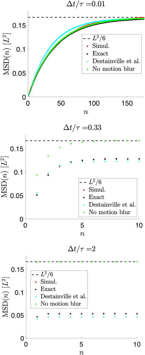
FIGURE 3. Mean-squared displacements (MSDs) of measured positions for a Brownian particle in a 1D box for $\text{Δ}t/\tau$ = 0.01 (top plot), 0.33 (middle plot), and 2 (bottom plot) with $\text{Δ}t=\text{Δ}{t}_{\text{open}}$. Each panel shows the MSD for the simulated data (red), the exact expression from Eq. 22 (black), the expression from [18] stated in Eq. 25 (cyan), and the expression without the effect of motion blur from Eq. 24 (green). The horizontal black dashed line marks $L^2/6$, the limit reached for $\text{Δ}t/\tau \to 0$ and $n\to \infty$.

For $n{\pi }^2\text{Δ}t/4\tau \gg 1$, we immediately get from Eq. 22 that $\text{MSD}\left(n\right)\simeq 2\text{var}\left(x_{\text{msr}}\right)$, where $\text{var}\left(x_{\text{msr}}\right)$ is found in Eq. 18. Additionally, still in this limit, using Eq. 20 valid for $\text{Δ}{t}_{\text{open}}/\tau \ll 1$, we find that

$\text{MSD}\left(n\right)\to \frac{L^2}{6}\left(1-\frac{\text{Δ}{t}_{\text{open}}}{\tau }\right)\text{ for }n\text{ large}.(23)$

Thus, motion blur, described to lowest order in $\text{Δ}{t}_{\text{open}}/\tau$, reduces the asymptotic value of $\text{MSD}\left(n\right)$ by a factor $\left(1-\text{Δ}{t}_{\text{open}}/\tau \right)$ relatively to its value in the absence of motion blur (Figure 3).

Figure 3 also illustrates that both D and L, in principle, can be determined from data, provided that $\text{Δ}t<\tau$ and n is sufficiently large. If the first condition is not satisfied, information about D is lost, and the MSD essentially assumes its plateau value already for $n=1$. If, on the other hand, n is limited and $\text{Δ}t<\tau$, e.g., due to poor sampling of a particle’s trajectory, information about the confining domain is lost, since the particle, typically, does not encounter the boundaries in this case.

In the absence of motion blur and localization errors—i.e., if positions are recorded instantaneously with infinite precision—the MSD can be calculated exactly for all values of n directly from Eq. 13 (Figure 3) [22],

$\text{MSD}\left(n\right)=\langle {[x_{j+n}-x_j]}^2\rangle =\frac{L^2}{6}\left(1-\frac{96}{{\pi }^4}{\displaystyle \sum }_{p=0}^{\infty }\frac{\text{exp}[-{\left(\frac{\pi }{2}\left(1+2p\right)\right)}^2\frac{\text{Δ}t}{\tau }n]}{{\left(1+2p\right)}^4}\right).(24)$

Results for the MSD similar to our Eq. 22 were previously found by Destainville and Salomé [18] in order to improve analysis of data from [17]. Considering a fully open shutter ($\text{Δ}t=\text{Δ}{t}_{\text{open}}$), they elegantly arrived at an expression for the MSD by considering the lowest-order expansion of the correlation between the true positions by adjusting the characteristic time-scales to ensure that their expression obeys the correct scaling properties for short and longtime-scales. In our notation, their Eq. 8 reads²

${\text{MSD}}_{\text{Destainville}}\left(n\right)=\frac{L^2}{9}\frac{\tau }{\text{Δ}t}-\frac{L^2}{27}{\left(\frac{\tau }{\text{Δ}t}\right)}^2\left\{1-\text{exp}\left[-3\frac{\text{Δ}t}{\tau }\right]\right\}-\frac{L^2}{54}{\left(\frac{\tau }{\text{Δ}t}\right)}^2{e}^{-3n\frac{\text{Δ}t}{\tau }}\left\{e^{3\frac{\text{Δ}t}{\tau }}+e^{-3\frac{\text{Δ}t}{\tau }}-2\right\}.(25)$

This is similar, but not identical to Eq. 22, see Figure 3, likely because their parameters were chosen to produce the correct scaling properties from a single term, i.e., similar to our term with $p=0$ in Eq. 22. Moreover, for $n\to \infty$, the MSD reaches a plateau value equal to twice the measured variance, and keeping only the first term in the sum for the variance in Eq. 22 gives a more accurate expression for the plateau value than Eq. 25 when $\text{Δ}{t}_{\text{open}}/\tau >0.08$ (see Supplementary Figure S1). For analysis of data, they suggest to fit the measured MSD to a simpler expression (their Eq. 2) followed by an adjustment of the fitted parameters to account for the finite exposure time, rather than to fit directly with the MSD of Eq. 25. It is, however, simpler and more accurate to estimate D and L by fitting the measured MSDs with our exact expression, Eq. 22, using D and L as fitting parameters.

2.4 2D Brownian Motion Confined to a Disc

Another relevant case to consider is that of a Brownian particle confined to a 2D circular disc with radius $a=L/2$ and reflecting walls at the boundary. Without loss of generality, we let the disc be centered at the origin. In this case, the problem does not factorize into a component for each Cartesian coordinate. Instead, we write the particle’s position in polar coordinates as $\mathbf{r}=\mathbf{r}\left(r,\varphi \right)$ with $0\le r<a$ and $0\le \varphi <2\pi$. If particles are distributed uniformly over the disc, the probability density is in polar coordinates $p\left(r,\varphi \right)=r/\left(\pi a^2\right)$. The mean position is at the center, $\langle \mathbf{r}\rangle =\left(\mathrm{0,0}\right)$, in Cartesian coordinates, and the variance is

$\text{var}\left(\mathbf{r}\right)=\langle {\left(\mathbf{r}-\langle \mathbf{r}\rangle \right)}^2\rangle ={{{\displaystyle \int }}^{\text{}}}_0^{2\pi }d\varphi {{{\displaystyle \int }}^{\text{}}}_0^{a}dr{r}^{2}p\left(r,\varphi \right)=\frac{a^2}{2}.(26)$

For the case of Brownian motion confined to a 2D disc, the solution to the diffusion Fokker–Planck equation for the conditional probability density for the particle’s position $\mathbf{r}$ at time t, given it was ${\mathbf{r}}_0$ at time $t=0$, is, with closed boundary conditions at $r=a$ [22],

$P\left(\mathbf{r},t|{\mathbf{r}}_0,0\right)=\frac{1}{\pi a^2}+\frac{1}{\pi a^2}{\displaystyle \sum }_{\ell =-\infty }^{\infty }\text{cos}\left[\ell \left(\varphi -{\varphi }_0\right)\right]{\displaystyle \sum }_{m=1}^{\infty }\frac{{\alpha }_{\ell m}^2}{{\alpha }_{\ell m}^2-{\ell }^2}\text{exp}\left[-{\alpha }_{\ell m}^2\frac{t}{\tau }\right]\frac{J_{\ell }\left({\alpha }_{\ell m}\frac{r}{a}\right)J_{\ell }\left({\alpha }_{\ell m}\frac{r_0}{a}\right)}{J_{\ell }{\left({\alpha }_{\ell m}\right)}^2},(27)$

where $\tau =a^2/D$ and ${\alpha }_{\ell m}>0$ is the mth positive root, $J_{\ell }^{\prime }\left({\alpha }_{\ell m}\right)=0$, of the derivative of the Bessel function of the first kind of order $\ell$, $J_{\ell }$. The zeros are arranged in ascending order of magnitude: $0<{\alpha }_{\ell 1}<{\alpha }_{\ell 2}<\dots$.

2.4.1 Variance of Positions Recorded With Motion Blur, for a Brownian Trajectory on a 2D Disc

For the 2D case, we define the measured position similarly to Eq. 1. The variance of the measured positions is calculated in a manner similar to the 1D case, and the result is

$\text{var}\left({\mathbf{r}}_{\text{msr}}\right)=\frac{8a^2}{{\left(\text{Δ}{t}_{\text{open}}\right)}^2}{\displaystyle \sum }_{m=1}^{\infty }\left\{\frac{\tau \text{Δ}{t}_{\text{open}}}{{\alpha }_{1m}^4\left({\alpha }_{1m}^2-1\right)}-\frac{{\tau }^2\left(1-\text{exp}\left[-{\alpha }_{1m}^2\frac{\text{Δ}{t}_{\text{open}}}{\tau }\right]\right)}{{\alpha }_{1m}^6\left({\alpha }_{1m}^2-1\right)}\right\}.(28)$

For details of the calculation, see Supplementary Material. This exact expression agrees with simulated data (Figure 4A–C) of particles undergoing Brownian motion confined to a 2D disc and subject to motion blur (Figure 4D).

FIGURE 4

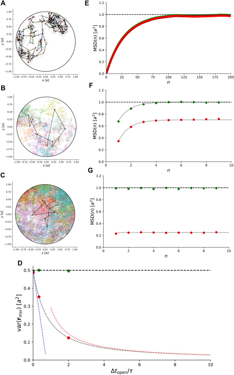
FIGURE 4. Simulations of 2D Brownian motion confined to a circular domain with radius a. (A)–(C) Simulated trajectories for $\text{Δ}t/\tau$ = 0.01, 0.33, and 2, respectively, and $\text{Δ}t=\text{Δ}{t}_{\text{open}}$. The measured positions, which are affected by motion blur, are indicated with black dots connected by dashed lines. The underlying positions visited by the particle during each frame in the time-lapse movie are shown with different color for each frame, plotted on top of each other with the latest frame on top. (D) Variance for the same values of the ratio $\text{Δ}t/\tau$ as in panels (A)–(C) (red dots). Dotted curves: the exact result for the variance in Eq. 28 (black), the approximate result in Eq. 29 valid for $\text{Δ}{t}_{\text{open}}\ll \tau$ (blue), and the approximate result in Eq. 30 valid for $\text{Δ}{t}_{\text{open}}\gg \tau$ (red). Horizontal black dashed line: variance = $a^2/2$, the value for $\text{Δ}{t}_{\text{open}}/\tau \to 0$. (E)–(G) Mean-squared displacements (MSDs) for $\text{Δ}t/\tau$ = 0.01, 0.33, and 2, respectively, and with $\text{Δ}t=\text{Δ}{t}_{\text{open}}$. Colored dots: measured positions excluding (green) and including (red) the effect of motion blur. Dotted lines through colored dots: exact results excluding (Eq. 32) and including (Eq. 31) the effect of motion blur. The horizontal black dashed line marks $a^2$, the limit reached for $\text{Δ}t/\tau \to 0$ and $n\to \infty$.

In the limit where the exposure time, $\text{Δ}{t}_{\text{open}}$, is negligible compared to the characteristic time, τ,

$\text{var}\left({\mathbf{r}}_{\text{msr}}\right)\simeq 4a^2{\displaystyle \sum }_{m=1}^{\infty }\frac{1}{{\alpha }_{1m}^2\left({\alpha }_{1m}^2-1\right)}=\frac{a^2}{2}\left(1-\frac{4}{3}\frac{\text{Δ}{t}_{\text{open}}}{\tau }\right),(29)$

which is equal to the variance of a particle’s positions under instantaneous (and noise-free) recording (see Supplementary Material).

On the other hand, for $\text{Δ}{t}_{\text{open}}\gg \tau$, we get

$\text{var}\left({\mathbf{r}}_{\text{msr}}\right)\simeq \frac{7}{24}\frac{a^2\tau }{\text{Δ}{t}_{\text{open}}}.(30)$

To arrive at this expression, we evaluated the relevant sum following [25], see Supplementary Material.

These limiting behaviors are also indicated in Figure 4D. Qualitatively, the implications of the variance of particle positions confined to a 2D circular domain and with positions recorded using finite exposure time are similar to the case of a particle confined to a box.

2.4.2 MSD of Positions Recorded With Motion Blur, for a Brownian Trajectory on a 2D Disc

A calculation similar to that for the 1D case yields the MSD of a 2D Brownian trajectory on a disc (Supplementary Material),

$\begin{array}{l}\text{MSD}\left(n\right)=2\text{var}\left({\mathbf{r}}_{\text{msr}}\right)\\ -8a^2{\left(\frac{\tau }{\text{Δ}{t}_{\text{open}}}\right)}^2{\displaystyle \sum }_{m=1}^{\infty }\frac{e^{-{\alpha }_{1m}^2}\frac{\left(n+\text{Δ}{t}_{\text{open}}/\text{Δ}t\right)\text{Δ}t}{\tau }}{{\alpha }_{1m}^6\left({\alpha }_{1m}^2-1\right)}{\left(1-e^{{\alpha }_{1m}^2\text{Δ}{t}_{\text{open}}/\tau }\right)}^2.\end{array}(31)$

This expression is exact for all values of $\text{Δ}{t}_{\text{open}}/\tau$ and $n\ge 1$, and it agrees with simulation results for particles undergoing 2D Brownian motion confined to a disc (Figure 4E–G). To our knowledge, the literature contains no similar explicit expression for the $\text{MSD}$ under these circumstances, let alone an exact one. When fitting Eq. 28 to a mean-squared displacement calculated from data, the sum converges rapidly. So, we give the first five values of ${\alpha }_{1m}$ for completeness: ${\alpha }_{11}=1.8412$, ${\alpha }_{12}=5.3314$, ${\alpha }_{13}=8.5363$, ${\alpha }_{14}=11.7060$, and ${\alpha }_{15}=14.8636$.

In the case of instantaneous and noise-free recording of positions, it has been shown that the MSD can be calculated from Eq. 27 [22, 25]. The result is

$\text{MSD}\left(n\right)=a^2\left(1-8{\displaystyle \sum }_{\ell =1}^{\infty }\text{exp}\left[-{\alpha }_{1\ell }^2\frac{n\text{Δ}t}{\tau }\right]\frac{1}{{\alpha }_{1\ell }^2\left({\alpha }_{1\ell }^2-1\right)}\right).(32)$

That is, Eq. 32 is the 2D version of Eq. 24, valid for instantaneous (and noise-free) sampling. We note that this expression is recovered from our result, Equation (31), in the limit of $\text{Δ}{t}_{\text{open}}/\tau \to 0$ (Supplementary Material). This expression also agrees with simulated data of a particle undergoing 2D Brownian motion confined to a disc, with instantaneous and noise-free recording of simulated positions (Figure 4E–G).

2.5 3D Brownian Motion Confined to a 3D Sphere

We now consider a Brownian particle confined to a 3D sphere with radius $a=L/2$. Similar to the 2D case confined to a circle, solutions to the diffusion equation factorize when expressed in spherical coordinates with the center of the sphere chosen as origin. Then, $\mathbf{r}=\mathbf{r}\left(r,\theta ,\varphi \right)$ with $0\le r<a$, $0\le \theta <\pi$, and $0\le \varphi <2\pi$. For particles distributed uniformly within the sphere, the probability density distribution in Cartesian coordinates is $p\left(x,y,z\right)=3/\left(4\pi a^3\right)$ for $x^2+y^2+z^2<a^2$. This becomes $p\left(r,\theta ,\varphi \right)=3r^2\text{sin}\theta /\left(4\pi a^3\right)$ in spherical coordinates. So, the variance is

$\text{var}\left(\mathbf{r}\right)=\langle {\mathbf{r}}^2\rangle ={{{\displaystyle \int }}^{\text{}}}_0^{\pi }d\theta {{{\displaystyle \int }}^{\text{}}}_0^{2\pi }d\varphi {{{\displaystyle \int }}^{\text{}}}_0^{a}drp\left(r,\theta ,\varphi \right)r^2=\frac{3}{4\pi a^3}{{{\displaystyle \int }}^{\text{}}}_0^{\pi }d\theta \text{sin}\theta {{{\displaystyle \int }}^{\text{}}}_0^{2\pi }d\varphi {{{\displaystyle \int }}^{\text{}}}_0^{a}dr{r}^4=\frac{3a^2}{5}.(33)$

The solution to the diffusion Fokker–Planck equation for the conditional probability density for the particle’s position $\mathbf{r}$ at time t, given it was ${\mathbf{r}}_0$ at time $t=0$, with closed boundary conditions at $r=a$, is [22]

$\begin{array}{l}P\left(\mathbf{r},{\mathbf{r}}^{\prime },t\right)=\\ \frac{3}{4\pi a^3}+\frac{2}{a^3}{\displaystyle \sum }_{\ell =0}^{\infty }{\displaystyle \sum }_{m=-\ell }^{\ell }{Y}_{\ell m}\left(\theta ,\varphi \right)Y_{\ell m}^{\text{*}}\left({\theta }^{\prime },{\varphi }^{\prime }\right){\displaystyle \sum }_{n=1}^{\infty }\frac{{\beta }_{\ell n}^2}{{\beta }_{\ell n}^2-\ell \left(\ell +1\right)}\text{exp}\left[-{\beta }_{\ell n}^2\frac{t}{\tau }\right]\frac{j_{\ell }\left({\beta }_{\ell n}\frac{r}{a}\right)j_{\ell }\left({\beta }_{\ell n}\frac{r^{\prime }}{a}\right)}{j_{\ell }{\left({\beta }_{\ell n}\right)}^2}.\end{array}(34)$

Here, $\tau =a^2/D$ and $j_{\ell }\left(x\right)=\sqrt{\pi /\left(2x\right)}{J}_{\ell +1/2}\left(x\right)$, where $j_{\ell }\left(x\right)$ is a spherical Bessel function of the first kind and $\ell$ is a positive integer. The functions $Y_{\ell m}\left(\theta ,\varphi \right)$ are spherical harmonics, and ${\beta }_{\ell n}$ are the (non-zero) zeros of the derivatives of the spherical Bessel functions, $j_{\ell }^{\prime }\left({\beta }_{\ell n}\right)=0$, which are arranged in ascending order of magnitude $0<{\beta }_{\ell 1}<{\beta }_{\ell 2}<\dots$.

2.5.1 Variance of Positions Recorded With Motion Blur, for a Brownian Trajectory in a 3D Sphere

For the 3D case, we define once again the measured position similarly to Eq. 1. The calculation of the variance of the measured positions is similar to the 1D case leading to the result (for details, see Supplementary Material),

$\text{var}\left({\mathbf{r}}_{\text{msr}}\right)=\frac{12a^2}{{\left(\text{Δ}{t}_{\text{open}}\right)}^2}{\displaystyle \sum }_{n=1}^{\infty }\left[\frac{\tau \text{Δ}{t}_{\text{open}}}{{\beta }_{1n}^4\left({\beta }_{1n}^2-2\right)}-\frac{{\tau }^2\left(1-\text{exp}\left[-{\beta }_{1n}^2\frac{\text{Δ}{t}_{\text{open}}}{\tau }\right]\right)}{{\beta }_{1n}^6\left({\beta }_{1n}^2-2\right)}\right].(35)$

Figure 5A–C show trajectories of particles undergoing confined Brownian motion in a 3D sphere. The exact result for the variances of the measured positions agrees with the simulated data (Figure 5D). When the exposure time is small compared to the characteristic timescale, i.e., $\text{Δ}{t}_{\text{open}}/\tau \ll 1$, the variance of the measured positions is approximately

$\text{var}\left({\mathbf{r}}_{\text{msr}}\right)\simeq \frac{3a^2}{5}\left(1-\frac{5}{3}\frac{\text{Δ}{t}_{\text{open}}}{\tau }\right).(36)$

FIGURE 5

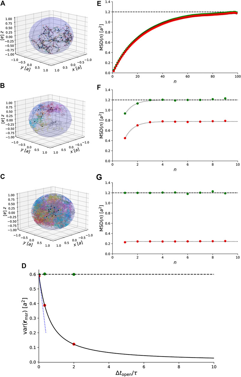
FIGURE 5. Simulations of 3D Brownian motion confined to a spherical domain with radius a. (A)–(C) Simulated trajectories for $\text{Δ}t/\tau$ = 0.01, 0.33, and 2, respectively, and $\text{Δ}t=\text{Δ}{t}_{\text{open}}$. The measured positions including the effect of motion blur are indicated (black dots connected by dashed lines). The underlying positions visited by the particle during each frame in the time-lapse movie are shown with different color for each frame, plotted on top of each other with the latest frame on top. (D) Variance for the same values of the ratio $\text{Δ}t/\tau$ as in panels (A)–(C) (red dots). Dotted curves: the exact result for the variance in Eq. 35 (black), the approximate result in Eq. 36 valid for $\text{Δ}{t}_{\text{open}}\ll \tau$ (blue). Horizontal black dashed line: variance = $3a^2/5$, the value for $\text{Δ}{t}_{\text{open}}/\tau \to 0$. (E)–(G) Mean-squared displacements (MSDs) for $\text{Δ}t/\tau$ = 0.01, 0.33, and 2, respectively, and with $\text{Δ}t=\text{Δ}{t}_{\text{open}}$. Colored dots: measured positions excluding (green) and including (red) the effect of motion blur. Dotted lines through colored dots: exact results excluding (Eq. 38) and including (Eq. 37) the effect of motion blur. The horizontal black dashed line marks $6a^2/5$, the limit reached for $\text{Δ}t/\tau \to 0$ and $n\to \infty$.

Details of the calculation are presented in Supplementary Material.

2.5.2. MSD of Positions Recorded With Motion Blur, for a Brownian Trajectory in a 3D Sphere

A calculation similar to the one done for the 1D case gives the MSD for a 3D Brownian trajectory confined within a 3D sphere. The result is

$\begin{array}{c}\text{MSD}\left(n\right)=2\text{var}\left({\mathbf{r}}_{\text{msr}}\right)-12a^2\frac{{\tau }^2}{{\left(\text{Δ}{t}_{\text{open}}\right)}^2}{\displaystyle \sum }_{m=1}^{\infty }\frac{1}{{\beta }_{1m}^6\left({\beta }_{1m}^2-2\right)}\text{exp}\left[-{\beta }_{1m^{\prime }}^2\frac{n\text{Δ}t+\text{Δ}{t}_{\text{open}}}{\tau }\right]\\ \times {\left(1-e^{{\beta }_{1m^{\prime }}^2\text{Δ}{t}_{\text{open}}/\tau }\right)}^2.\end{array}(37)$

This expression is exact for all values of $\text{Δ}{t}_{\text{open}}/\tau$ and $n\ge 1$. Figure 5E–G show excellent agreement between Eq. 37 and the MSD calculated from simulated Brownian trajectories confined within a 3D sphere and imaged with motion blur. This constitutes another result that, to our knowledge, does not exist in the literature. As for the 1D and 2D cases, the sum converges rapidly, which is useful knowledge when applying the expression in a fit to experimental data. So, for practical completeness and the reader’s convenience, we again give the first five values of ${\beta }_{1n}$: ${\beta }_{11}=2.08158$, ${\beta }_{12}=5.94037$, ${\beta }_{13}=9.20584$, ${\beta }_{14}=12.4044$, and ${\beta }_{15}=15.5792$.

In the absence of motion-blur—i.e., in the case of instantaneous recording of exact positions—the MSD can be calculated directly from the propagator in Eq. 34 with the result [22]

$\text{MSD}\left(n\right)=a^2\left(\frac{6}{5}-12{\displaystyle \sum }_{m=1}^{\infty }\text{exp}\left[-{\beta }_{1m}^2\frac{n\text{Δ}t}{\tau }\right]\frac{1}{{\beta }_{1m}^2\left({\beta }_{1m}^2-2\right)}\right).(38)$

This result is also indicated in Figure 5E–G.

2.6 2D Anisotropic Brownian Motion Confined to a 2D Disc

So far, we only considered isotropic Brownian motion, i.e., with identical diffusion coefficients in all directions. Now, we discuss the implications of confinement on anisotropic Brownian motion that is imaged with motion blur. For simplicity, we restrict the discussion to anisotropic 2D Brownian motion confined to a disc. In this case, the probability density is described by a Fokker–Planck equation, which in Cartesian coordinates reads (compare with Eq. 2)

$\begin{array}{c}\frac{\partial P\left(x,y,t|x_0,y_0,t_0\right)}{\partial t}=\left(D_x\frac{{\partial }^2}{\partial x^2}+D_y\frac{{\partial }^2}{\partial y^2}\right)P\left(x,y,t|x_0,y_0,t_0\right)\\ =D_x\left(\frac{{\partial }^2}{\partial x^2}+\frac{D_y}{D_x}\frac{{\partial }^2}{\partial y^2}\right)P\left(x,y,t|x_0,y_0,t_0\right).\end{array}(39)$

Here, we have chosen Cartesian coordinates with axes along the two primary axes of the diffusion tensor without loss of generality. The isotropic case is recovered for $D_x=D_y$. The boundary condition due to the confinement is no flux perpendicular to the boundary, i.e., at $x^2+y^2=a^2$, and the initial condition is $P\left(x,y,t_0|x_0,y_0,t_0\right)=\delta \left(x-x_0\right)\delta \left(y-y_0\right)$. If we scale the y-coordinate as $y=\widehat{y}\sqrt{D_y/D_x}$ and let $D=D_x$, we get

$\begin{array}{c}\frac{\partial P\left(x,\widehat{y},t|x_0,{\widehat{y}}_0,t_0\right)}{\partial t}\\ =D\left(\frac{{\partial }^2}{\partial x^2}+\frac{{\partial }^2}{\partial {\widehat{y}}^2}\right)P\left(x,\widehat{y},t|x_0,{\widehat{y}}_0,t_0\right),\end{array}(40)$

and the boundary condition becomes $x^2/a^2+{\widehat{y}}^2/b^2=1$, where $b=a\sqrt{D_x/D_y}$. So, the problem of anisotropic diffusion in circular confinement is equivalent to isotropic diffusion confined to an elliptical domain.³

By introducing elliptic coordinates and rewriting Eq. 40 in these coordinates, a solution for the propagator can be found by separation of temporal and spatial variables, exactly as for the other cases considered above. The solution for the spatial part is given in terms of Mathieu functions [26], but the structure of these functions complicates a compact analytic solution.

Instead, we simulated trajectories of anisotropic Brownian motion confined to a 2D disc and recorded them with $\text{Δ}t=\text{Δ}{t}_{\text{open}}$ (Materials and Methods). We did this for various values of the ratios $D_y/D_x$ and $\text{Δ}t/\tau$. Here, we define $\tau \equiv a^2/D_x$. Figure 6A–C shows examples of such trajectories for $D_y/D_x=10$. The variance of the measured positions for various values of $\text{Δ}t/\tau$ and $D_y/D_x$ are shown in Figure 6D, including and excluding the effect of motion blur. Figure 6E–G show the corresponding MSDs for the same values of $\text{Δ}t/\tau$ and $D_y/D_x$.

FIGURE 6

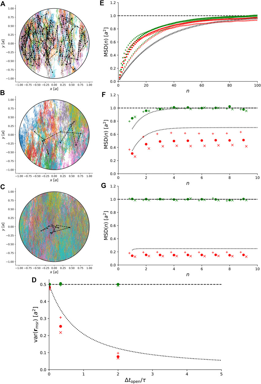
FIGURE 6. Simulations of 2D anisotropic Brownian motion confined to a circular domain with radius a. (A)–(C) Simulated trajectories for $\text{Δ}t/\tau$ = 0.01, 0.33, and 2, respectively, with $\text{Δ}t=\text{Δ}{t}_{\text{open}}$, $\tau =a^2/D_x$, and $D_y/D_x=10$. The measured positions including the effect of motion blur are indicated (black dots connected by dashed lines). The underlying positions visited by the particle during each frame in the time-lapse movie are shown with different color for each frame, plotted on top of each other with the latest frame on top. (D) Variance for the same values of the ratio $\text{Δ}t/\tau$ as in panels (A)–(C). Plusses are for $D_y/D_x=2$, dots for $D_y/D_x=5$, and crosses for $D_y/D_x=10$. Color: measured positions excluding (green) and including (red) the effect of motion blur. Dotted curve: the exact result for the variance for isotropic Brownian motion $D_y/D_x=1$ (Eq. 28). Horizontal black dashed line: $a^2/2$, corresponding to the variance for a uniform distribution on a circle. (E)–(G) Mean-squared displacements (MSDs) for $\text{Δ}t/\tau$ = 0.01, 0.33, and 2, respectively, and with $\text{Δ}t=\text{Δ}{t}_{\text{open}}$. The symbols and the colors are as in (D), but are slightly offset for clarity. Dotted lines through colored symbols: Exact results for isotropic Brownian motion, $D_y/D_x=1$, excluding (Eq. 32) and including (Eq. 31) the effect of motion blur. The horizontal black dashed line marks $a^2$, i.e., twice the variance for a uniform distribution on a circle.

For comparison, Figure 6D–G also show the exact theoretical results for variance and MSD for isotropic Brownian motion, i.e., for $D_x=D_y$. The variances obtained from simulations including motion blur fall below the theory for isotropic Brownian motion and more so for increasing ratios of $D_y/D_x$ and intermediate ratios of $\text{Δ}{t}_{\text{open}}/\tau$, since the motion blur there effectively limits the observed positions of the particle. Notice that the MSD for $\text{Δ}t/\tau =0.01$ and finite time lags exceeds the theory for isotropic Brownian motion, since motion blur is limited and consequently allow observation of the longer displacements of a particle with $D_y>D_x$ relatively to those of a particle with $D_y=D_x$ (Figure 6E). This effect flips as $\text{Δ}t/\tau$ increases and motion blur in conjunction with $D_y>D_x$ causes the observed MSDs to fall below the theory for isotropic Brownian motion (Figure 6F,G).

This illustrates that for anisotropic Brownian motion, the coupling between confinement and motion blur is non-trivial and care must be taken to rule out anisotropic diffusion before our exact results for isotropic Brownian motion are used to interpret experimental results.

3 Discussion

In this work, we presented exact formulas for the variance and MSD of positions of a particle undergoing Brownian motion in confining spaces. These formulas remain valid when random Gaussian localization errors make true and recorded positions differ, provided that these localization errors are independently and identically distributed, which often is the case or may be assumed. To account for the localization error, our formulas should be offset merely by $2{\sigma }_{\text{loc}}^2$ for each coordinate contributing to the quantity of interest, the variance, or the MSD (Section 4.5). This localization error may be found using established methods [3, 6].

We assumed normal Brownian motion throughout this article, and our formulas are guaranteed to apply only for such motion. On the other hand, we used only second moments of distributions, so results may in principle generalize to other cases with finite second moment if they exist. In some cases, particles may exhibit more complicated, types of motion, such as sub-diffusion due to interactions with other molecules in a membrane or “hop-diffusion”: particles may be almost confined to nano-domains but “hop” between neighboring domains [17, 27].

Other complication we ignored. Particles experience increased viscous drag near surfaces, as described by Faxén [28], and may experience attractive depletion forces near surfaces if many smaller particles—e.g., macromolecules—are present. Results of simulations and experiments, in which these and other effects are, respectively, simulated or suspected, can now be compared to the exact statistics given above for cases of steric confinement alone.

Additionally, while the approach described here delivers results for individual molecules, precision on estimates for parameters requires long trajectories [4]. In applications, the number of data points in a trajectory depends, e.g., on the fluorescent label and may be much lower than that used in our simulations. In such cases, one may compromise as regards true single-molecule results and average over a sample of several or many molecules to improve statistics of results obtained with our formulas [4].

Our formulas should facilitate that as much information as possible can be extracted about the mobility of the particles and the confining domains. To do this, one should account for the fact that the estimated MSD-values are correlated, since they are obtained from the same trajectory. This makes optimal fitting to MSDs complicated [16]. Additionally, in the present case of confined Brownian motion, such correlations most likely also depend on the position of the particle relative to the boundaries. Our formulas could, in principle, also facilitate a more accurate use of the MSD as a basis for classifying the type of motion [27].

The covariance-based estimator (CVE) introduced and demonstrated in [6, 7, 29] is an attractive alternative; however, away from surfaces, it estimates the bulk value of D, does that even from short segments of the trajectory, and does this optimally, provided its SNR = $\sqrt{D\text{Δ}t}/{\sigma }_{\text{loc}}>1$ [6, 7]. So, our exact MSD is probably best used with experimental MSD-values as a fairly simple way to gauge deviation from bulk behavior as function of time-scale of measurement.

In conclusion, there is still work to do in the field of analysis of single-molecule and single-particle trajectories. Trajectories of self-propelled particles, e.g., are better understood as persistent random motion. Tools for analysis of such trajectories with accounting for motion blur and/or effects of confinement would amount to quite an oeuvre even for the simplest model, the Ornstein-Uhlenbeck process, we predict, based on [30], though methods developed in [31, 32] may help. Here, we have exhausted a small fraction of this field with exact formulas for the variances and MSDs for simple Brownian motion, valid when particle positions are recorded using finite exposure time, which is the typical case by far. These formulas should help researchers to get the most out of their data for motion of Brownian particles and the domains that confine them, e.g., for particles diffusing in cell membranes [4, 10, 17].

4 Materials and Methods

4.1 Simulations

Equation (3) describes the propagator $P\left(x,t|x_0,t_0\right)$ of the diffusion equation. It shows how to propagate free diffusion between fixed points in time, $t_j=j\text{Δ}t$ (j integer): given that the particle is at position $x_j$ at time $t_j$, simply draw a random number from a Gaussian distribution with zero mean and variance ${\sigma }^2=2D\text{Δ}t$ and add this random number to $x_j$. The sum is $x_{j+1}$. Thus, we simulate time-lapse sampled positions on a trajectory of Brownian motion by iterating

$x_{j+1}=x_j+\sqrt{2D\text{Δ}t}{\eta }_j,(41)$

where ${\left({\eta }_j\right)}_{j=\mathrm{1,2},\dots }$ is the normalized Gaussian white noise, i.e., for all $i,j$, $\langle {\eta }_j\rangle =0$ and $\langle {\eta }_i{\eta }_j\rangle ={\delta }_{ij}$. The displacements $\text{Δ}{x}_j=x_j-x_{j-1}$ are consequently by construction independent and normally distributed, with zero mean and variance ${\sigma }^2=2D\text{Δ}t$. Since independent, they are uncorrelated, $\langle \text{Δ}{x}_i\text{Δ}{x}_j\rangle =0$ for $i\ne j$; compare Eqs. 4–6.

4.2 Simulation of Free Brownian Motion With Motion Blur

We simulate the effect of motion blur by dividing the time-lapse $\text{Δ}t$ into a large number of sub-intervals of duration $\delta t$. Instead of iterating Eq. 41 with $\text{Δ}t$, we iterate it with $\delta t$ in $\text{Δ}t\text{'}\text{s}$ place and time-average the resulting positions over each time-lapse of duration $\text{Δ}t$. These averages equal the measured positions described in Eq. 1, except we approximated its integral with a sum over many terms.

4.3 Simulation of Brownian Motion in Confinement

For free diffusion, it was possible to simulate a trajectory by sampling random numbers from the probability density function in Eq. 3, as the function is a Gaussian. In principle, one could simulate diffusion of a particle diffusing between walls at $x=0$ and $x=L$ in a similar manner by drawing random number from the probability density distribution in Eq. 13. For $\sqrt{2D\text{Δ}t}\ll L$, which is the case in our simulations, it is much simpler just to iterate Eq. 41 with two extra conditions: if an iteration makes $x_{j+1}<0$, this position is replaced by its image reflected in the box-wall at $x=0$, i.e., with $-x_{j+1}>0$, and iteration is continued from this value, which is recorded as the position at time $t_{j+1}$. Entirely analogous, if an iteration makes $x_{j+1}>L$, this position is replaced by its image reflected in the box-wall at $x=L$, i.e., with $2L-x_{j+1}<L$, and iteration is continued from this value, which is recorded as the position at time $t_{j+1}$.

This protocol assumes that $x_{j+1}<-L$ and $x_{j+1}>2L$ never occurs, which is why we assume $\sqrt{2D\text{Δ}t}\ll L$; it ensures that these inequalities occur with negligible probability. Not that this is crucial. The methods of mirrors just described are easily generalized to handle the occurrence of said inequalities.

For more complex geometries, e.g., the 2D disc, closed boundaries can be implemented as described in [33]. For the case of anisotropic Brownian motion confined to a 2D disc, the implementation of the reflecting boundary is complicated. So, we implemented it by exploiting that anisotropic Brownian motion confined to a circular domain is equivalent to isotropic Brownian motion confined to an elliptical domain, see Section 2.6. With this transformation, the reflecting boundary conditions may be implemented, essentially, as described in [33]. After generating such transformed trajectories, we scaled positions back to original space.

4.4 Calculation of the Mean-Squared Displacement From Data

We estimated the mean-squared displacement from the simulated positions with [7]

${\text{MSD}}_{\text{data}}\left(n\right)=\frac{1}{N-n}{\displaystyle \sum }_{j=1}^{N-n}{\left(x_{j+n}-x_j\right)}^2,(42)$

where $x_j$, $j=\mathrm{1,2,3},\dots N$, are the measured or simulated positions in the trajectory.

4.5 Influence of Localization Errors

If the expected number of photons collected from the label on a particle is constant in time, the standard deviation, ${\sigma }_{\text{loc}}$, of the localization error does not depend on time. Since images are uncorrelated, so are the localization errors in different frames in the movie of the particle. Consequently, the localization error can be accounted for by adding $2{\sigma }_{\text{loc}}^2$ to any value of the variance and/or the MSD for a position coordinate. Here, the factor 2 is the number of positions involved in calculation of a variance or MSD. That is, for the variances and the MSDs stated for the 1D case in Section 2.3, simply add $2{\sigma }_{\text{loc}}^2$ to all results, for the results for the 2D cases in Sections 2.4and2.6, add $4{\sigma }_{\text{loc}}^2$, and for the results for the 3D case in Section 2.5, add $6{\sigma }_{\text{loc}}^2$.

Data Availability Statement

The raw data supporting the conclusions of this article will be made available by the authors, without undue reservation.

Author Contributions

KM and JP conceived the idea, did the research, and wrote the first draft of the manuscript. HF wrote the second version of the manuscript.

Funding

This work was supported by the Novo Nordisk Foundation Challenge Programme (NNF16OC0022166 to KM and HF).

Conflict of Interest

The authors declare that the research was conducted in the absence of any commercial or financial relationships that could be construed as a potential conflict of interest.

Supplementary Material

The Supplementary Material for this article can be found online at: https://www.frontiersin.org/articles/10.3389/fphy.2020.583202/full#supplementary-material.

Footnotes

¹Note that by time-lapse, we mean the inverse frame rate: the lapse between, e.g., the start of consecutive frames. The “time-lapse” between the end of recording of one frame and the beginning of the next frame we call dead time.

²In [18], the definition of τ is $L^2/12$, i.e., a factor of 3 smaller than our definition of τ.

³If we had started out with the slightly more general case of confinement to an ellipse with axes parallel to the axes of the diffusion tensor, we would also land on this result after rescaling.

References

1. Schmidt T, Schütz GJ, Baumgartner W, Gruber HJ, Schindler H. Imaging of single molecule diffusion. Proc Natl Acad Sci Unit States Am (1996) 93:2926–9. doi:10.1073/pnas.93.7.2926

CrossRef Full Text | Google Scholar

2. Manley S, Gillette JM, Patterson GH, Shroff H, Hess HF, Betzig E, et al. High-density mapping of single-molecule trajectories with photoactivated localization microscopy. Nat Methods (2008) 5:155–7. doi:10.1038/nmeth.1176

PubMed Abstract | CrossRef Full Text | Google Scholar

3. Mortensen KI, Churchman LS, Spudich JA, Flyvbjerg H. Optimized localization analysis for single-molecule tracking and super-resolution microscopy. Nat Methods (2010) 7:377–81. doi:10.1038/nmeth.1447

PubMed Abstract | CrossRef Full Text | Google Scholar

4. Arnspang EC, Sengupta P, Mortensen KI, Jensen HH, Hahn U, Jensen EBV, et al. Regulation of plasma membrane nanodomains of the water channel aquaporin-3 revealed by fixed and live photoactivated localization microscopy. Nano Lett (2019) 19:699–707. doi:10.1021/acs.nanolett.8b03721

PubMed Abstract | CrossRef Full Text | Google Scholar

5. Ruthardt N, Lamb DC, Bräuchle C. Single-particle tracking as a quantitative microscopy-based approach to unravel cell entry mechanisms of viruses and pharmaceutical nanoparticles. Mol Ther (2011) 19:1199–211. doi:10.1038/mt.2011.102

PubMed Abstract | CrossRef Full Text | Google Scholar

6. Vestergaard CL, Blainey PC, Flyvbjerg H. Optimal estimation of diffusion coefficients from single-particle trajectories. Phys Rev E (2014) 89:022726. doi:10.1103/PhysRevE.89.022726

CrossRef Full Text | Google Scholar

7. Vestergaard CL, Pedersen JN, Mortensen KI, Flyvbjerg H. Estimation of motility parameters from trajectory data. Eur Phys J Spec Top (2015) 224:1151–68. doi:10.1140/epjst/e2015-02452-5

CrossRef Full Text | Google Scholar

8. Clausen MP, Arnspang EC, Ballou B, Bear JE, Lagerholm BC. Simultaneous multi-species tracking in live cells with quantum dot conjugates. PloS One (2014) 9. doi:10.1371/journal.pone.0097671

PubMed Abstract | CrossRef Full Text | Google Scholar

9. Schütz GJ, Kada G, Pastushenko VP, Schindler H. Properties of lipid microdomains in a muscle cell membrane visualized by single molecule microscopy. EMBO J (2000) 19:892–901. doi:10.1093/emboj/19.5.892

PubMed Abstract | CrossRef Full Text | Google Scholar

10. Kure JL, Andersen CB, Mortensen KI, Wiseman PW, Arnspang EC. Revealing plasma membrane nano-domains with diffusion analysis methods. Membranes (2020) 10:314. doi:10.3390/membranes10110314

CrossRef Full Text | Google Scholar

11. Adebiyi A, Soni H, John TA, Yang F. Lipid rafts are required for signal transduction by angiotensin ii receptor type 1 in neonatal glomerular mesangial cells. Exp Cell Res (2014) 324:92–104. doi:10.1016/j.yexcr.2014.03.011

PubMed Abstract | CrossRef Full Text | Google Scholar

12. Helms JB, Zurzolo C. Lipids as targeting signals: lipid rafts and intracellular trafficking. Traffic (2004) 5:247–54. doi:10.1111/j.1600-0854.2004.0181.x

PubMed Abstract | CrossRef Full Text | Google Scholar

13. Raghu H, Sodadasu PK, Malla RR, Gondi CS, Estes N, Rao JS. Localization of uPAR and MMP-9 in lipid rafts is critical for migration, invasion and angiogenesis in human breast cancer cells. BMC Canc (2010) 10:647. doi:10.1186/1471-2407-10-647

CrossRef Full Text | Google Scholar

14. Vestergaard CL. Optimizing experimental parameters for tracking of diffusing particles. Phys Rev E (2016) 94:022401. doi:10.1103/PhysRevE.94.022401

PubMed Abstract | CrossRef Full Text | Google Scholar

15. Berglund AJ. Statistics of camera-based single-particle tracking. Phys Rev E (2010) 82:011917. doi:10.1103/PhysRevE.82.011917

CrossRef Full Text | Google Scholar

16. Michalet X, Berglund AJ. Optimal diffusion coefficient estimation in single-particle tracking. Phys Rev E (2012) 85:061916. doi:10.1103/PhysRevE.85.061916

CrossRef Full Text | Google Scholar

17. Ritchie K, Shan XY, Kondo J, Iwasawa K, Fujiwara T, Kusumi A. Detection of non-brownian diffusion in the cell membrane in single molecule tracking. Biophys J (2005) 88:2266–77. doi:10.1529/biophysj.104.054106

PubMed Abstract | CrossRef Full Text | Google Scholar

18. Destainville N, Salomé L. Quantification and correction of systematic errors due to detector time-averaging in single-molecule tracking experiments. Biophys J (2006) 90:L17–L19. doi:10.1529/biophysj.105.075176

PubMed Abstract | CrossRef Full Text | Google Scholar

19. Grebenkov DS. Nmr survey of reflected Brownian motion. Rev Mod Phys (2007) 79:1077–137. doi:10.1103/RevModPhys.79.1077

CrossRef Full Text | Google Scholar

20. Risken H. The Fokker–Planck equation: methods of solution and applications. Berlin: Springer (1984).

CrossRef Full Text | Google Scholar

21. Bullerjahn JT, von Bülow S, Hummer G. Optimal estimates of self-diffusion coefficients from molecular dynamics simulations. J Chem Phys (2020) 153:021101. doi:10.1063/5.0008312

PubMed Abstract | CrossRef Full Text | Google Scholar

22. Bickel T. A note on confined diffusion. Phys Stat Mech Appl (2007) 377:24–32. doi:10.1016/j.physa.2006.11.008

CrossRef Full Text | Google Scholar

23. Wong WP, Halvorsen K. The effect of integration time on fluctuation measurements: calibrating an optical trap in the presence of motion blur. Optic Express (2006) 14:12517–31. doi:10.1364/OE.14.012517

CrossRef Full Text | Google Scholar

24. Mitra PP, Halperin BI. Effects of finite gradient-pulse widths in pulsed-field-gradient diffusion measurements. J Magn Reson, Ser A (1995) 113:94–101. doi:10.1006/jmra.1995.1060

CrossRef Full Text | Google Scholar

25. Riseborough PS, Hänggi P. Diffusion on surfaces of finite size: Mössbauer effect as a probe. Surf Sci (1982) 122:459–73. doi:10.1016/0039-6028(82)90096-6

CrossRef Full Text | Google Scholar

26. McLachlan N. Theory and application of Mathieu functions. Oxford, UK: Clarendon Press (1947).

CrossRef Full Text | Google Scholar

27. Clausen MP, Lagerholm BC. Visualization of plasma membrane compartmentalization by high-speed quantum dot tracking. Nano Lett (2013) 13:2332–7. doi:10.1021/nl303151f

PubMed Abstract | CrossRef Full Text | Google Scholar

28. Happel J, Brenner H. Low Reynolds number hydrodynamics. Upper Saddle River, NJ:Prentice-Hall (1965).

CrossRef Full Text | Google Scholar

29. Vestergaard CL, Blainey PC, Flyvbjerg H. Single-particle trajectories reveal two-state diffusion-kinetics of hOGG1 proteins on DNA. Nucl Acids Res (2018) 46:2446–58. doi:10.1093/nar/gky004

PubMed Abstract | CrossRef Full Text | Google Scholar

30. Pedersen JN, Li L, Gradinaru C, Austin RH, Cox EC, Flyvbjerg H. How to connect time-lapse recorded trajectories of motile micro-organisms with dynamical models in continuous time. Phys Rev E (2016) 94:062401. doi:10.1103/PhysRevE.94.062401

PubMed Abstract | CrossRef Full Text | Google Scholar

31. Brueckner DB, Fink A, Schreiber C, Roettgermann PJF, Raedler JO, Broedersz CP. Stochastic nonlinear dynamics of confined cell migration in two-state systems. Nat Phys (2019) 15:595–601. doi:10.1038/s41567-019-0445-4

CrossRef Full Text | Google Scholar

32. Brueckner DB, Ronceray P, Broedersz CP. Inferring the dynamics of underdamped stochastic systems. Phys Rev Lett (2020) 125:058103. doi:10.1103/PhysRevLett.125.058103

PubMed Abstract | CrossRef Full Text | Google Scholar

33. Volpe G, Gigan S, Volpe G. Simulation of the active brownian motion of a microswimmer. Am J Phys (2014) 82:659–64. doi:10.1119/1.4870398

CrossRef Full Text | Google Scholar