 Acep Purqon
 Jamaludin
94% of researchers rate our articles as excellent or good
Learn more about the work of our research integrity team to safeguard the quality of each article we publish.
Find out more
ORIGINAL RESEARCH article
Front. Phys., 19 January 2021
Sec. Social Physics
Volume 8 - 2020 | https://doi.org/10.3389/fphy.2020.574770
This article is part of the Research TopicFrom Physics to Econophysics and Back: Methods and InsightsView all 31 articles
A stock market represents a large number of interacting elements, leading to complex hidden interactions. It is very challenging to find a useful method to detect the detailed dynamical complex networks involved in the interactions. For this reason, we propose two hybrid methods called RMT-CN-LPAm+ and RMT-BDM-SA (RMT, random matrix theory; CN, complex network; LPAm+, advanced label propagation algorithm; BDM, block diagonal matrix; SA, simulated annealing). In this study, we investigated group mapping in the S&P 500 stock market using these two hybrid methods. Our results showed the good performance of the proposed methods, with both the methods demonstrating their own benefits and strong points. For example, RMT-CN-LPAm+ successfully identified six groups comprising 485 involved nodes and 17 isolated nodes, with a maximum modularity of 0.62 (identified more groups and displayed more maximum modularity). Meanwhile, RMT-BDM-SA provided useful detailed information through the decomposition of matrix C into
Physics is the study of the structure and dynamics of various systems that exist in nature. In its current form, the scope of the subject encompasses not only physical systems, but all complex systems. A complex system is one that comprises parts or agents interacting with each other to produce a new macroscopic collective behavior without a central control [1]. Such systems are easily observed in econophysics and social physics (sociophysics).
An example of a complex system in the field of econophysics is the financial market, especially the stock market. It has numerous investors and companies interacting with each other, exchanging assets in their possession to determine the best price for each of them. In general, there are several scientific reasons for physicists to be interested in learning the dynamics that underlie the stock market system [1].
In physical systems, the basis for each agents interactions with another in the system is known; for example, the electrostatic system, where the interaction between charges is based on Coulomb forces. However, in the stock market, the mechanisms underlying the interactions between each agent are not yet clearly known [2]. A starting point for the study of stock markets can be the analysis of the correlation between stocks. A review of the relations between agents in the system is the easiest way to determine the linearity of such relationships in the system without the need to know their underlying cause. From this efficient market hypothesis, it follows that all agents in the stock market get information simultaneously, and every time the information enters the stock market, the stocks respond with changes in the price of the shares so that the share prices reflect the current market conditions. Therefore, the correlation between the stocks can be seen from fluctuations in the share prices.
Recently, a few excellent studies have been published on community detection based on local information and dynamic expansion [3]; the application of random matrix theories, and graphs or networks [4, 5]. Because each method has its strong points and weaknesses, we propose to combine the strong points and reduce the limitations or the weak points and use a combination of these methods for finding the correlations between agents in the stock market system. For example, group mapping involves two different approaches: advanced label propagation algorithm (LPAm+) and simulated annealing (SA). Both methods have limitations, as shown in a few studies. Our objective was to combine LPAm+ with a complex network (CN) and SA with a block diagonal matrix (BDM) for improved effectiveness. LPAm+ with CN determines the group of each node based on the most frequent label of their neighbor. Meanwhile, SA with BDM provides the dual benefit of constructing a block diagonal matrix and finding a global minimum, showing an annealing concept similar to that seen while constructing a crystal. However, the correlations still contain noise and need to be preprocessed using an efficient method. One of the eligible candidates to clean the stock data and remove noise is the random matrix theory (RMT).
As stock market conditions change all the time, the correlations among shares also change. Therefore, the correlations contained in the stock market do not fully describe the relationship between actual stocks. This implies the possibility of noise in the correlation between stocks [6]. In this study, we investigated a method for separating noise from data that contain real information using RMT. The main concept behind RMT is a comparison of the distribution of eigenvalues and eigenvectors in the correlation matrix data owned by a random correlation matrix. Any part of the data that does not display the characteristics of a random correlation matrix is the part that actually contains the real information (non-noise) of the stock market system; vice versa, if any part of the data displays characteristics similar to a random correlation matrix, it is noise.
An analysis of the eigenvalues and eigenvectors of the stock matrix correlation structure has shown that a few of the largest eigenvector components are localized; for example, components with the greatest contribution to each eigenvector are found in the same sector [2]. However, these results are not sufficiently significant to be adopted as a method for analyzing groups in the stock market because each eigenvector is not independent of each other (a few sectors overlap in one eigenvector). Moreover, during the analysis of eigenvector components, only a few vector components were observed to have the greatest contribution [7]. Therefore, in this study, another approach was used to analyze the stock market groups and a few candidates were found. We used a CN as the first approach and a BDM as the second.
In the CN approach, each share in the stock market is seen as a node, and the correlation between the shares is analogous to the connecting side between the nodes. To form a stock market network, the LPAm+ method is used, which determines the group (community) label of a node based on the majority of its neighbor labels; nodes with the same label are considered to be in the same group or community. Conversely, in the BDM approach, the stock correlation matrix is converted to a BDM, where each block represents a group in the stock market; the method is chosen to create the BDM as an SA algorithm, which mimics the annealing process in crystal formation. The data used in the study were the daily closing price of the shares listed on the S&P 500 from January 1, 2007 to October 28, 2016.
Our purpose was to: 1) generate a correlation filtering data filtering program using the RMT method; 2) develop a program for mapping the groups in the stock market using the LPAm+ and SA algorithms, and 3) compare the results of the mapped groups in the stock market by employing the CN approach using LPAm+ (namely RMT-CN-LPAm+) and the BDM approach using the SA algorithm (namely RMT-BDM-SA).
The application of RMT assumes a matrix whose elements are random or not bound to one another. A random matrix has zero average value and one variance [8]. RMT was first introduced by Wigner to explain energy-level statistics in complex quantum systems. Wigner created a matrix model with random elements to explain the Hamiltonian mechanics of a heavy nucleus that fit the experimental results [9]. In complex quantum systems, RMT predictions can explain all the possibilities that can occur in system [10]; in subsequent developments, it was concluded that parts incompatible with RMT predictions can provide clues about the interactions that underlie the system [8].
In the late 1990s, Laloux et al. and Pelrou et al. applied RMT to correlation data based on changes in stock prices on the American stock markets [6]. Subsequently, several physicists tried to apply RMT to different stock markets. The results showed similarity to the extent that RMT could identify the noise part contained in the correlation data between stocks, and proved that most of the stock data followed the random correlation matrix pattern [2, 7, 10–12]. RMT can distinguish between noise and the real information part by comparing the data held in a random correlation matrix. When a part of the data does not follow the properties or characteristics of a random correlation matrix, it is ensured that the particular part contains real information from the stock market system; and if a part of data has the same characteristics as a random correlation matrix, then that part is noise.
There are several characteristics of a random correlation matrix used in RMT. For example, if A is a random matrix with dimensions
When the values
Here,
A network can be defined as a set of objects called vertices (nodes or vertices); the relationships between vertices are called lines or sides (edges or links) [13]. Suppose a network
The degree of a network is defined as the number of sides passing through a node. The degree of node i can be calculated using the following equation:
Then, the total degree of a network can be calculated as follows:
The shortest path that connects two vertices is commonly called the geodesic path. Take for example, a matrix D whose elements are geodesic distances between vertices i and j or
The node betweenness parameter measures the effect of a node in a network by counting the several geodesic paths through that node. Mathematically, it is expressed as
Here,
The cluster coefficient parameter measures the tendency of n from node i to become a group or cluster in a network. The cluster coefficient of node i is calculated by the ratio between the number of sides (
Then, the average cluster coefficient of each node, also called the network cluster coefficient, is calculated as follows:
The quality of the grouping of communities in a network can be measured from the relationship between the intra-community and inter-community nodes. When the relationships between the intra-community nodes are dense and those between the inter-community nodes are rare, then the grouping of networks, as well as the parameters that measure the relationships, are considered good. This is called modularity; a term first introduced by Newman [14]. The extent of modularity in a network can be calculated using the following equation:
Here,
Based on their degree distribution, networks can be classified into two most common types: exponential and scale-free. In exponential networks, the degree distribution follows the Poisson distribution, which means that most of the nodes in the network have the same degree (they are homogeneous). In scale-free networks, the distribution of degrees in heterogeneous networks follows the power-law distribution, that is, most vertices have a small degree; a few or a small proportion of them have a large degree. Examples of exponential and scale-free networks can be seen in Ref. [15] and their distribution in Ref. [16].
Noh proposed a diagonal block matrix model and demonstrated that for stocks that belong to one group, the diagonals of the formed correlation matrix have a value of one and the remaining entries have the value zero
Here,
Kim and Jeong proposed an optimization of the BDM by analyzing the correlation between stocks as a force that binds to particles (in this case, stocks) [7]. Because of the binding force between the shares, there is total energy in the system. The equation that calculates the system energy is given in Eq. 11, and the most stable BDM form is obtained when the energy in the system is the minimum. An example of the BDM calculated by Kim and Jeong using the New York Stock Exchange (NYSE) stock data for the 1993–2003 period can be found in Ref. [7].
Here,
To separate noise from the information in the correlation data through several stages, namely, during the distribution comparison between the correlation matrix C and the random correlation matrix R to calculate the correlation of each share, the return for each stock is calculated as
Here,
where
In matrix representations, it is expressed by
where G is a matrix
To compare the eigenvalue distribution of the correlation matrix C and the random correlation matrix R, the eigenvector interpretation of the correlation matrix C that is outside the predicted RMT tests the stability of each eigenvector of the correlation matrix C. First, we divide the stock price data (matrix S) into two parts (the first half
A matrix can be decomposed into a linear combination of from a collection of matrices. To find a noise-free correlation matrix, the decomposition is expressed by
where N is the number of shares and λ is the eigenvalue of the C matrix sorted.
In the CN approach, the C correlation matrix (which is noise free) can be treated as an adjacency matrix [_Jeong_and_Kim_2005] demonstrated that to find a clear definition for each group (community) in the network, a weighted network needs to be chosen for the group analysis in the stock market [7]. Because the value of the elements in the
LPAm+ is a method for developing the label propagation algorithm (LPA) method. The main idea of the LPA method is to determine the community label of a node based on the majority of labels from its neighbors; the nodes that have the same label are grouped into one community (group) [18]. At the beginning of the algorithm, different (unique) labels are given for each node; then, during propagation, a node changes its label to follow the majority of its neighboring labels, and in case of a tie (there is more than one label with the same number), the label is determined randomly. The iteration stops if there is no longer a label propagation process in the network. In mathematical form, the label update process can be written according to the following equation:
Because there is a random aspect to the labeling during series conditions as described previously, this LPA method does not produce a unique solution for each run. As a result, more than one community structure can exist even if they originate from the same initial conditions. Therefore, the LPA method is generally performed several times and a community structure that has the greatest modularity value is taken. The main advantage of the LPA method is its very high speed compared with other methods [18].
Barber and Clark modified the LPA method by increasing the monotonous value of the rising modularity in each iteration [19]. The modularity equation can be rearranged as follows:
The aforementioned equation denotes the separation of the terms containing the label of node x from the previous modularity equation. To maximize the modularity value, the writer must maximize the
However, the LPAm method still has a shortcoming of possibly getting trapped in the local maximum in the modularity space; thus, Liu and Murata modified the LPAm method by applying agglomeration techniques to combine each of the two groups (communities) and avoid any changes in values. The modularity then chooses which results in the largest change in modularity value. The combination of these methods is called LPAm+ [20].
Regardless of the first local maximum value, the LPAm steps are repeated to reach the next local maximum value. The aforementioned two methods (LPAm and agglomeration) are repeated until there are no more modularity changes.
To find the stock arrangement that provides the most system energy, the SA algorithm is used in Monte Carlo simulations to avoid brute force. The SA algorithm was first introduced by Metropolis. Furthermore, SA was first applied to the optimization issue by Kirkpatrick et al. to avoid local drinking conditions [21]. This algorithm is analogous to the annealing (cooling) process that is applied while producing glassy materials (comprising crystalline grains).
The annealing process can be defined as a regular or constant temperature drop on a previously heated solid object until it reaches the ground state or freezing point. The temperature is reduced continuously and carefully so that a thermal balance is attained at each level. If the temperature is not reduced stepwise, the solid object acquires structural defects due to the formation of only optimal local structures. This type of process that produces only an optimal local structure is called rapid quenching. The search for a solution with SA is similar to the hill-climbing concept where the solution tends to change continuously until the final temperature is reached.
In the SA algorithm, we introduce the concept of annealing to the formation of crystals in optimization problems. The objective function, that is to search for the minimum value in the optimization problem, is compared with the energy of the material in the case of the annealing process. Then, a control parameter, which is the temperature, is used for each iteration.
The SA algorithm uses the concept of a neighborhood search or local search in each iteration to find conditions that provide the lowest objective function. For each iteration, if the surrounding conditions (in the case of a BDM, the composition of shares) provides an objective function value smaller than the original objective function, then the initial condition is updated (the condition of the neighbor is set as the new initial condition). However, when the condition of the neighbor outputs a value greater than the original objective function, the result can still be accepted (the initial condition is enhanced by the condition of the neighbor) with certain conditions of probability.
Classical particle probability is used in this case, which follows Maxwell-Boltzmann statistics
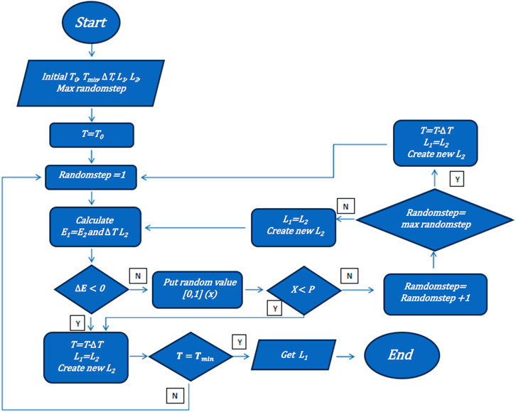
FIGURE 1. Flowchart of the simulated annealing (SA) algorithm to form a block diagonal matrix (BDM). The most stable BDM is obtained when the energy in the system is of the minimum value. To find the most stable BDM and avoid the local minimum, we propose to combine it with simulated annealing, bringing the concept of annealing to the formation of crystals in optimization problems.
As mentioned in the previous section, the correlation value between shares has no fixed over time, and a plot was drawn for three different conditions of the stock correlation data. The first is the correlation matrix extracted from the 2007 to 2016 data (black line), the second is the correlation matrix for the data from 2007 to 2012 (green line), and the third is or the data from 2012 to 2016 (red line) using Eq. 12 through Eq. 15. The results are shown in Figure 2. According to the figure, there is an increase in the correlation coefficient between the stocks. The average correlation coefficient between the shares in the data for the periods 2007‒2012 and 2012‒ 2016 is 0.3832 and 0.2642, respectively. Then, for the whole period (2007‒2016), the average correlation coefficient is 0.3451.
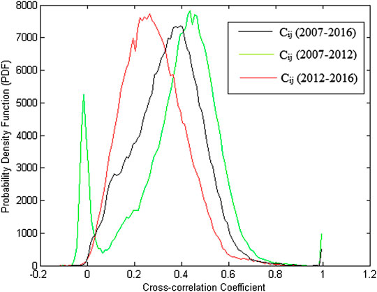
FIGURE 2. Distribution of correlation coefficients of matrix C at three different times in the S&P 500 daily stock price data for the period of January 1, 2007 until October 28, 2016. The black color is for the total period 2012‒2016 and it is decomposed into the green one for the period 2007‒2012 and the red one for the period 2012‒2016. It shows how the black one contributes to the different distribution of the green and red ones.
Next, the distribution of the C correlational matrix was compared with that of the R random correlation matrix. The results in Figure 3 show that the distribution of the R matrix follows a Gaussian trend, whereas the C matrix has a positive leaning distribution, indicating that the relationship between the stocks on the S&P 500 dominant correlates with each other compared to those who have anti-correlation relationships.
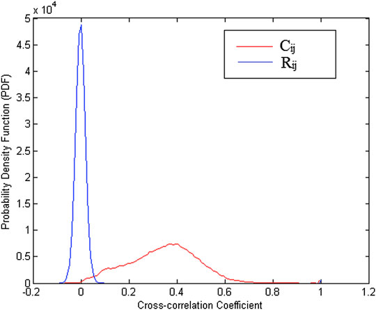
FIGURE 3. The Probability Density Function (PDF) of the correlation coefficient C matrix and the R matrix. The red color shows the distribution of the C matrix, and the blue one indicates the distribution of the R matrix on the S&P 500 daily stock price data for the period of January 1, 2007 until October 28, 2016. It clearly shows the different distribution groups separately for the correlation coefficient C matrix and R.
Figure 4 shows the eigenvalue distributions of the C matrix and the random correlation R matrix following Eq. 1. It can be seen that most (97%) eigenvalues of the C matrix are in the vulnerable boundary of the random R matrix, which indicates that most of the stock data are noise. Only 3% eigenvalues of the C matrix are outside the boundary of the random matrix R, and represent the real information from the stock market. The largest eigenvalue produced is 185.38, which is more than 90 times the upper limit of the eigenvalue matrix R (
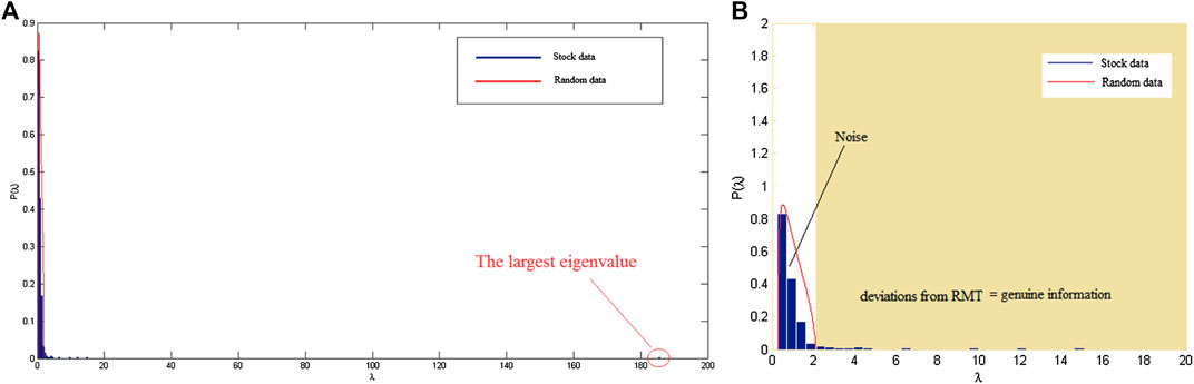
FIGURE 4. The distribution of eigenvalues from the C matrix and the R matrix. The blue color represents the distribution of the eigenvalues of the matrix C, and the red one shows the distribution of the eigenvalues of the matrix R on the S&P 500 daily stock price data for the period of January 1, 2007 until October 28, 2016. (A) eigenvalue in the scale for λ of 1‒200 and (B) The eigenvalue in the zoomed scale for λ of 1-20.
Apart from looking at the distribution of eigenvalues from the C correlation matrix, we also tested for the presence of noise in the data by looking at the distribution of the eigenvector components. Figure 5 shows the different distributions of eigenvector components outside and within the boundary of a random matrix (using RMT ). The eigenvector component within the boundary of the random matrix in Figure 5C follows the Gaussian distribution as given in Eq. 3. This shows that this part is noise, whereas the distribution of the eigenvector component outside the boundary of the random matrix in Figures 5A,B is heavy or leaning toward one side.
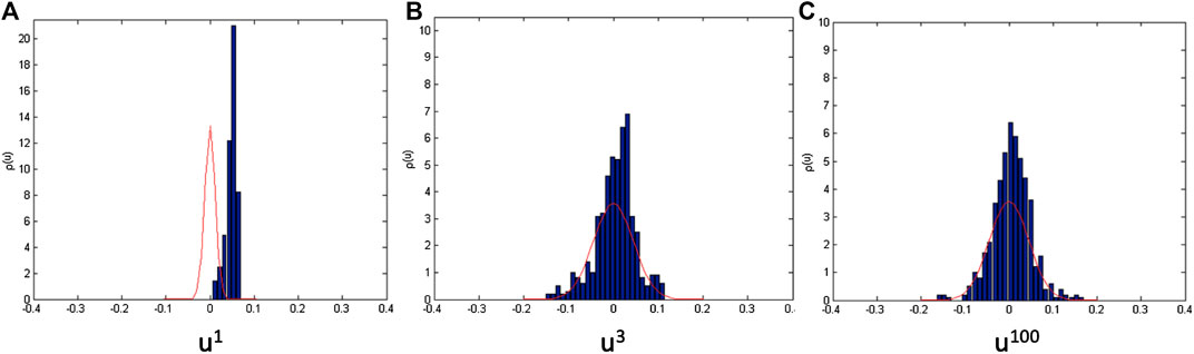
FIGURE 5. Comparison among the distribution of eigenvector components. For example, (A) is the largest
After successfully distinguishing between noise and data containing real information, we then identified each C eigenvalue that was outside the boundary of the random matrix. The uniqueness of the largest eigenvalue can be observed easily when compared with other eigenvalues because of its greater value than others, as seen in Figures 4, 5A, which shows that all the components of the eigenvector are positive. This demonstrates that the largest eigenvalue has a very significant influence on the dynamics of the stock market, commonly referred to as the market-wide effect [2].
To test the assumption that the largest eigenvalue has a market-wide effect, a comparison between the projections of the eigenvector components was calculated using Eq. 22 with an S&P 500 index value. Figure 6 shows that the projections of the largest eigenvector components and S&P 500 have the same movement patterns. These results reinforce that the largest eigenvalue is a representation of the movement of the stock market itself. The equation is as follows:
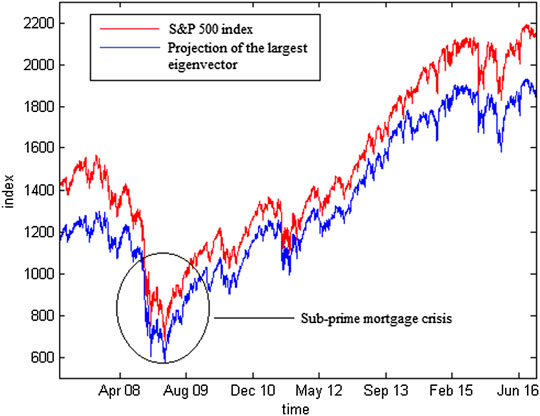
FIGURE 6. To validate how good the Eigen vectors, we can perform a comparison of projections of the largest eigenvector component (blue) from matrix C with the S&P 500 index (red) on the S&P 500 daily share price data for the period of January 1, 2007 until October 28, 2016. This indicates that the method mainly follows the patterns successfully.
After successfully identifying the largest eigenvalue, we also performed identification on other eigenvalues that are still outside the boundary of the random matrix. However, before doing that, the largest eigenvalue must be removed first owing to its market-wide effects. As the results in the previous section have shown, the largest eigenvalue is a representation of the market movement itself and has a very significant effect on the components of other eigenvectors and constrains the other eigenvectors [2]. To eliminate the market-wide effects, an ordinary least square is expressed as follows:
where
The greater the value of an eigenvector component in its eigenvector, the greater is its contribution to the eigenvector. Figure 7 shows the values of each component of the eigenvectors
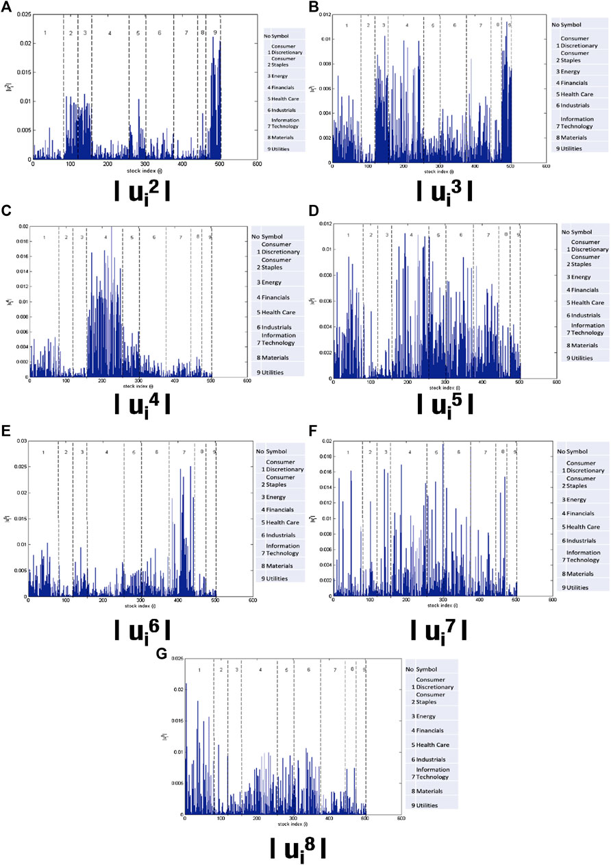
FIGURE 7. There are many information for each Eigen vectors. Some sectors overlap in several Eigen vectors. This indicates that we require a method to reveal community detection. The vector component of
After an analysis of the eigenvector components, it can be concluded that the groups identified are not yet comprehensive owing to the absence of sectors such as energy, materials, industrials, or consumer staples. This is because during the analysis of the eigenvectors, only the components with the greatest value are noted. Therefore, we cannot use only this method for group identification in the stock market. For the next analysis, we used a CN approach and BDM to identify groups in the stock market.
The results of mapping the stability of the eigenvectors of the C matrix can be seen in Figure 8. The results not only show that only the largest eigenvectors are stable over time but also reinforce previous results that eigenvector analysis cannot be used to determine groups in the stock market because only stable eigenvectors can be interpreted [23].
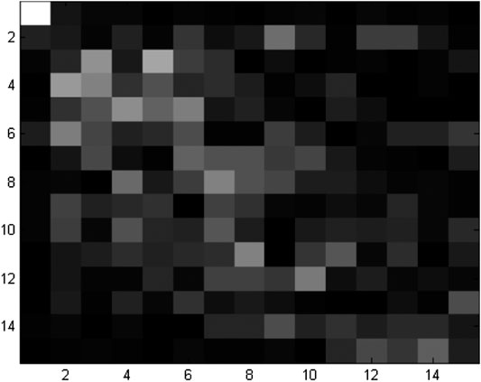
FIGURE 8. Stability of the eigenvectors from the largest eigenvectors (
From the results of the RMT method, it is evident that the stock market data contains not only noise but market-wide effects also; therefore, before analyzing the stock correlation data with CNs and the BDM, it must be cleaned from noise and market-wide effects. Matrix decomposition is used for cleaning, where matrix C is decomposed into three parts, namely market-wide (Cm), group (Cg), and noise (Cr), using Eq. 24. To be used as an adjacency A matrix in CNs and BDM analysis, only (Cg) is used. The equation is as follows:
Here,
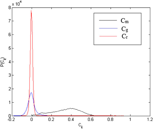
FIGURE 9. Matrix decomposition shows successfully decompose the group into three different parts. Distribution of Cm (black), Cg (blue), and Cr (red) on the S&P 500 daily share price data for the period of January 1, 2007 until October 28, 2016. This indicates that the method successfully shows the decomposition and contribution from each part.
In a non-weighted network, the determination of the boundary value is very important because each different boundary value forms a different group structure. If the selected boundary value is too small, all the nodes are connected, which means there is only one large group, and if the chosen boundary value is too large, only a small number of nodes are still connected in the network; most of them are isolated.
Therefore, to determine the boundary value in this study, four parameters were considered: the number of groups formed, number of vertices, number of sides, and average cluster coefficient [5, 11]. Figure 10 shows that the optimal boundary value is 0.05.
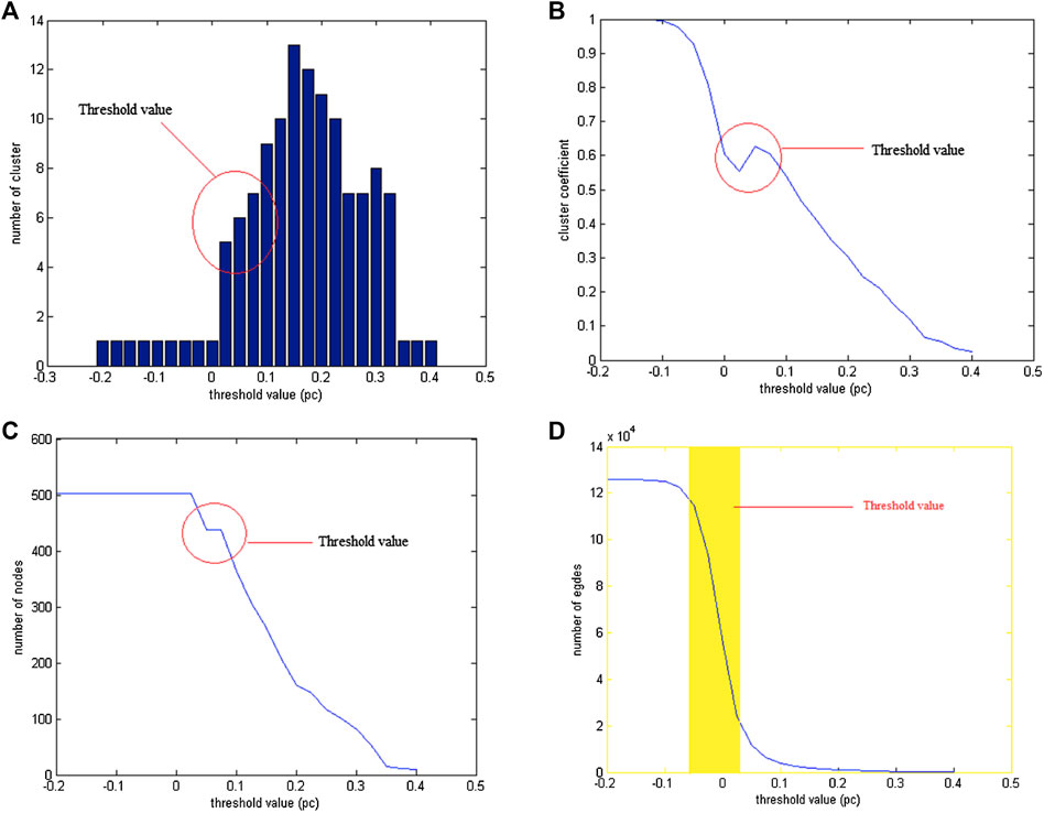
FIGURE 10. The value (A) number of clusters formed, (B) number of vertices, (C) cluster coefficients and (D) number of sides when boundary values vary from
The LPAm+ program on the S&P 500 network successfully identified the groups on the network. As many as six groups were observed, with the number of involved nodes reaching up to 485 out of a total 502 nodes (17 nodes were isolated from the network) and the maximum modularity value obtained was 0.6164.
The results obtained with LPAm+ show that the shares that belong to the same group are dominated by certain sectors (according to the results of the eigenvector analysis with RMT). Group mapping with LPAm+ can be visualized using Gephi software. The results obtained using the Gephi software are slightly different than those after using the LPAm+ method. In Gephi, there are six large clusters (groups) of the stock market network with a total of 483 (96%) nodes out of the total, 5579 sides, and a modular value of 0.619 (there is a difference of 0.003 with the LPAm+ results). Figure 11 shows the results of the animation using Gephi.
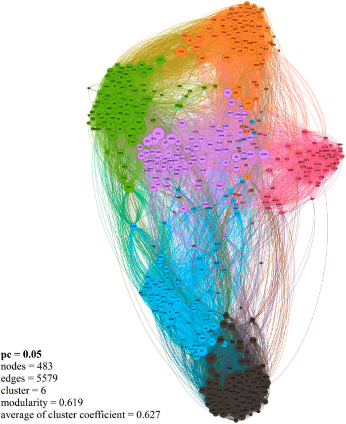
FIGURE 11. The method successfully performs community detection. The S&P 500 stock market network using Gephi software, there are six main clusters, cluster 1 (black) is dominated by the financial sector, cluster 2 (pink) is dominated by the information technology sector, cluster 3 (orange) is dominated by the energy sector, industrial and materials, cluster 4 (green) is dominated by the consumer staples, utilities, and industry sectors; cluster 5 (blue) is dominated by the consumer discretionary sector, and finally cluster 6 (purple) is dominated by the health care sector.
The results obtained using the SA algorithm and the Cg correlation matrix data show accordance with the concept of the BDM, namely the condition of the stock arrangement that provides the minimum system energy from group blocks in the correlation matrix.
In the SA algorithm, if the initial arrangement of the selected
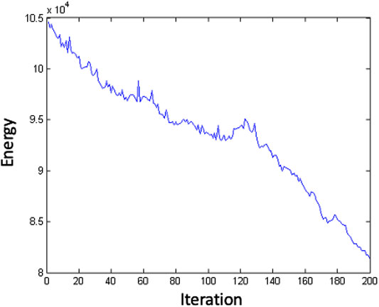
FIGURE 12. How energy decrease by iteration in Simulated annealing method results, for example with the initial guess set
Figure 13 shows the result obtained when the initial stock layout guess
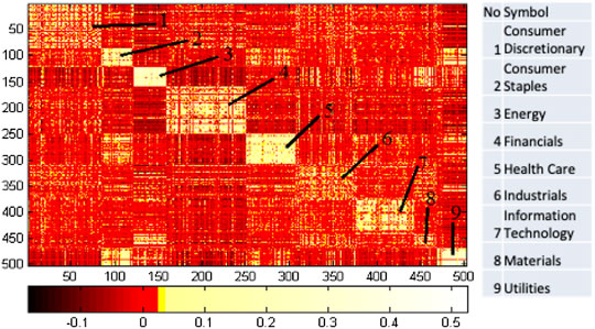
FIGURE 13. The community detection results from the Cg correlation matrix mapping using the stock structure generated by the Simulated Annealing (SA) algorithm with parameters
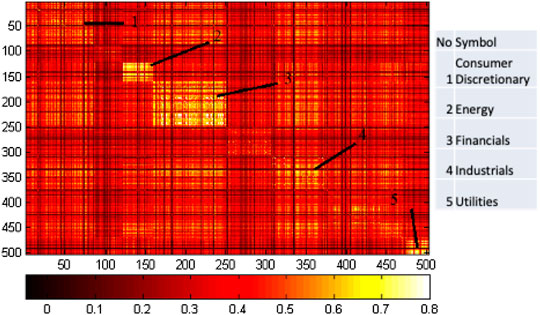
FIGURE 14. Community detection results from the Cg + Cm correlation matrix mapping with the same stock structure as in Figure 13. The sectors are group 1 consumer, 2 energy, 3 financials, 4 industrials, and 5 utilities.
We investigated complex networks in the S&P 500 stock market using two approaches, namely, a CN approach using an LPAm+ algorithm and a BDM approach using an SA algorithm. Before applying the two approaches, the data of the C stock correlation matrix were filtered using the RMT. RMT succeeded in separating the noise from non-noise data and showed that most of the data contained in the correlation matrix C were noise; an analysis of the distribution of eigenvector components in the RMT indicated that stock movements were driven by groups where each group was dominated by a particular sector. We called this analysis as simply RMT-CN-LPAm+ and RMT-BDM-SA.
In the first approach, the noise-free correlation matrix and market-wide(Cg) effects were analyzed using the CN approach with a threshold value of 0.05 and an LPAm+ network structure comprising six main groups with 485 out of a total 502 nodes involved (17 nodes were isolated from the network) and an obtained modularity value of 0.62. Then, in the second approach, which is a BDM with the same data, namely Cg using a simulated annealing algorithm, the stock structure provided a minimum energy system, and from this arrangement, nine groups of shares were produced. The decomposition of matrix C into Cm (market-wide), Cg (group), and Cr (noise) was also accomplished. The combination provides useful information to identify group classifications.
The difference between RMT-CN-LPAm+ and RMT-BDM-SA results is that in RMT-CN-LPAm+, a group contains not only the shares of the same sector but also of other minority sectors, whereas in RMT-BDM-SA, a group contains shares of the same sector. The second difference is that in MT-CN-LPAm+, a few shares still remain that have not joined any group, whereas in RMT-BDM-SA, not all shares have a group. In general, both hybrid methods successfully show good performance to reveal detailed community detections.
The original contributions presented in the study are included in the article/Supplementary Material, further inquiries can be directed to the corresponding author.
All authors listed have made a substantial, direct, and intellectual contribution to the work and approved it for publication.
The authors declare that the research was conducted in the absence of any commercial or financial relationships that could be construed as a potential conflict of interest.
The authors would like to thank Hawoong Jeong, Kim Soo Yong (KAIST), and many colleagues with valuable discussions.
1. Mantegna RN, Stanley HE. Introduction to econophysics: correlations and complexity in finance. Cambridge, United Kingdom, Cambridge University Press (1999).
2. Plerou V, Gopikrishnan P, Rosenow B, Amaral LAN, Guhr T, Stanley HE. Random matrix approach to cross correlations in financial data. Phys Rev (2002) 65:066126. doi:10.1103/physreve.65.066126
3. Luo Y, Wang L, Sun S, Xia C. Community detection based on local information and dynamic expansion. IEEE Access (2018) 7:142773–86.
4. Wang Z, Xia C, Chen Z, Chen G. Epidemic propagation with positive and negative preventive information in multiplex networks. IEEE Trans Cyber (2020) [Epub ahead of print]. doi:10.1109/itoec49072.2020.9141736
5. Zhang Z, Xia C, Chen S, Yang T, Chen Z. Reachability analysis of networked finite state machine with communication losses: a switched perspective. IEEE J Select Areas Commun (2020) 38:845–53. doi:10.1109/jsac.2020.2980920
6. Plerou V, Gopikrishnan P, Rosenow B, Nunes Amaral LA, Stanley HE. Universal and nonuniversal properties of cross correlations in financial time series. Phys Rev Lett (1999) 83:1471. doi:10.1103/physrevlett.83.1471
7. Kim D-H, Jeong H. Systematic analysis of group identification in stock markets. Phys Rev (2005) 72:046133. doi:10.1103/physreve.72.046133
9. Wigner E. On a class of analytic functions from the quantum theory of collisions annals of mathematics. Berlin, Heidelberg: Springer (1951).
10. Namaki A, Shirazi AH, Raei R, Jafari GR. Network analysis of a financial market based on genuine correlation and threshold method. Phys Stat Mech Appl (2011) 390:3835–41. doi:10.1016/j.physa.2011.06.033
11. Sharifi S, Crane M, Shamaie A, Ruskin H. Random matrix theory for portfolio optimization: a stability approach. Phys Stat Mech Appl (2004) 335:629–43. doi:10.1016/j.physa.2003.12.016
12. Utsugi A, Ino K, Oshikawa M. Random matrix theory analysis of cross correlations in financial markets. Phys Rev (2004) 70:026110. doi:10.1103/physreve.70.026110
13. Newman MEJ. The structure and function of complex networks. SIAM Rev (2003) 45:167–256. doi:10.1137/s003614450342480
14. Newman ME, Girvan M. Finding and evaluating community structure in networks. Phys Rev E (2004) 69:026113. doi:10.1103/physreve.69.026113
15. Jeong H. Complex scale-free networks. Phys Stat Mech Appl (2003) 321:226–37. doi:10.1016/s0378-4371(02)01774-0
16. Wang XF, Chen G. Complex networks: small-world, scale-free and beyond. IEEE Circuits Syst Magazine (2003) 3:6–20
17. Noh J. D. (2000). Model for correlations in stock markets. Phys Rev Rev E 61:5981. doi:10.1103/physreve.61.5981
18. Raghavan UN, Albert R, Kumara S. Near linear time algorithm to detect community structures in large-scale networks. Phys Rev E (2007) 76:036106. doi:10.1103/physreve.76.036106
19. Barber MJ, Clark JW. Detecting network communities by propagating labels under constraints. Phys Rev (2009) 80:026129. doi:10.1103/physreve.80.026129
20. Liu X, Murata T. Advanced modularity-specialized label propagation algorithm for detecting communities in networks. Phys Stat Mech Appl (2010) 389:1493–1500. doi:10.1016/j.physa.2009.12.019
21. Kirkpatrick S, Gelatt CD, Vecchi MP. Optimization by simulated annealing. Science (1983) 220:671–80. doi:10.1126/science.220.4598.671
22. Dréo J, Pétrowski A, Siarry P, Taillard E. Metaheuristics for hard optimization: methods and case studies. Berlin, Germany: Springer Science & Business Media (2006).
Keywords: random matrix theory, complex networks, advanced label propagation algorithm, block diagonal matrix, simulated annealing, hybrid methods
Citation: Purqon A and Jamaludin (2021) Community Detection of Dynamic Complex Networks in Stock Markets Using Hybrid Methods (RMT‐CN‐LPAm+ and RMT‐BDM‐SA). Front. Phys. 8:574770. doi: 10.3389/fphy.2020.574770
Received: 21 June 2020; Accepted: 28 September 2020;
Published: 19 January 2021.
Edited by:
Siew Ann Cheong, Nanyang Technological University, SingaporeReviewed by:
Chengyi Xia, Tianjin University of Technology, ChinaCopyright © 2021 Purqon and Jamaludin. This is an open-access article distributed under the terms of the Creative Commons Attribution License (CC BY). The use, distribution or reproduction in other forums is permitted, provided the original author(s) and the copyright owner(s) are credited and that the original publication in this journal is cited, in accordance with accepted academic practice. No use, distribution or reproduction is permitted which does not comply with these terms.
*Correspondence: Acep Purqon, YWNlcEBmaS5pdGIuYWMuaWQ=
Disclaimer: All claims expressed in this article are solely those of the authors and do not necessarily represent those of their affiliated organizations, or those of the publisher, the editors and the reviewers. Any product that may be evaluated in this article or claim that may be made by its manufacturer is not guaranteed or endorsed by the publisher.
Research integrity at Frontiers
Learn more about the work of our research integrity team to safeguard the quality of each article we publish.