1. Introduction
Inequality in a society can broadly be categorized as inequality of condition or inequality of opportunity. The former refers to disparities in the current status of individuals, whether this be income, wealth or their ownership of different goods and services. The latter refers to disparities in the future potential of individuals. Typically, inequality of opportunity is inferred indirectly through its effects like education level and quality, health status and treatment by the justice system. Though the two types of inequality are interrelated, we are interested in the former type only in this survey. Therefore, in what follows, the term “inequality” will refer exclusively to inequality of condition.
We focus here on one aspect of inequality, viz., the measurement of inequality. Measuring inequality is important for answering a wide range of questions. For instance: is the income distribution more equal than what it was in the past? Are underdeveloped countries characterized by greater inequality than developed countries? Do taxes or other kinds of policy interventions lead to greater equality in the distribution of income or wealth? Since the way inequality is measured also determines how the above questions (among others) are answered, a rigorous discussion of the measurement of inequality is necessary (see, e.g., Refs. 1–5).
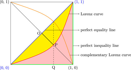
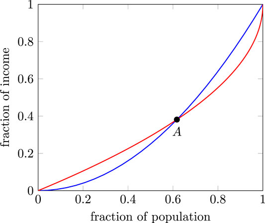
A tool that is indispensable in measuring income and wealth inequality is the Lorenz function and its graphical representation, the Lorenz curve (see Ref. 6). The Lorenz curve plots the percentage of total income earned by various portions of the population when the population is ordered by the size of their incomes. The Lorenz curve is typically depicted as a curve in the unit square with end points at and (see Figure 1).1 The 45° line is the line of perfect equality representing a situation where all individuals have the same income.
The Lorenz curve can be used, in a limited way, as a measure of inequality. Since the 45° line is the line of perfect equality, we can say that the “closer” a Lorenz curve is to the 45° line, the more equal is the income distribution. Unfortunately, this does not get us very far because Lorenz curves can intersect and hence, the Lorenz curves cannot be ranked unambiguously using the above criterion (see Ref. 7). We have more to say on this point in Section 2.
The existing literature sees two approaches to deal with the problem of intersecting Lorenz curves. The first is to consider ranking criterion that are “weaker” than this dominance criterion meaningful only for non-intersecting Lorenz curves (see Refs. 7–11). The pioneering work in this approach is Ref. 12 which suggested that there is an underlying notion of social welfare associated with any measure of income inequality. It is this concept with which we should be concerned. Furthermore, we should approach the question by considering directly the form of the social welfare function to be employed (see Ref. 13). This is a normative approach and is meaningful when we want to obtain a ranking of income distributions in order to infer something from the social welfare angle like whether “post-tax income is more equally distributed than pre-tax income”.
The second approach is to develop summary measures of inequality using the Lorenz functions (see Ref. 7 for details). Here, each Lorenz function is associated with a real number and these numbers are used to compare inequality across different income distributions. This is a descriptive approach where we quantify the difference in inequality between pairs of distributions (see Ref. 13).
An index of income inequality is therefore a scalar measure of interpersonal income differences within a given population. High income inequality means concentration of high incomes in the hands of few and is likely to compress the size of the middle class. A large and rich middle class contributes significantly to the well-being of a society in many ways. In particular, a large and rich middle class contributes in terms of high economic growth, better health status, higher education level, a sizable contribution to the country’s tax revenue and a better infrastructure, and more social cohesion resulting from fellow feeling. A society characterized with a small middle class and more persons away from the middle income group may lead to a strained relationship between the subgroups on the two sides of the middle class which can generate unrest (see Ref. 4). Hence, the need for identifying the magnitude of income inequality through different indices is of prime importance.
Except for the unique case of equality, where the Lorenz curve is trivially linear, the Lorenz function is typically nonlinear and it accommodates the essential features of the inequalities involved. However, most of the common inequality indices formulated and used so far studies some of the “average” properties of the Lorenz function. On the other hand, the established observations in statistical physics, for example in developing the Renormalization Group theory of phase transitions (see, e.g., Ref. 14) or the chaos theory (see, e.g., Ref. 15), strongly indicated the richness of the (nontrivial) fixed point structure (and also of the eigen vectors and eigen values for the linearized function near that fixed point) of such non-linear functions to comprehend the physical and mathematical process represented by such nonlinear functions. We noted earlier (see Ref. 1) that, while the Lorenz function has got trivial fixed points, a complementary Lorenz function has a non-trivial point corresponding to an inequality index called the Kolkata index, having several intriguing and useful properties.
Our primary focus in this survey will be on the Kolkata index as a measure of inequality. The Kolkata index, first introduced by Ref. 1 and later analyzed in Ref. 2 and in Ref. 3, is that proportion k of the population such that the proportion of income that we can associate with k is . Since no single summary statistic can reflect all aspects of inequality exhibited by the Lorenz curve, the importance of using alternative measures of inequality is universally acknowledged (see Ref. 7). We would also discuss two popular indices namely, the Gini coefficient or index (see Ref. 16) and the Pietra index (see Ref. 17). The Gini index is the ratio of the area between the 45° line and the Lorenz curve to the total area under the 45° line. Equivalently, the Gini index is twice the area between the Lorenz curve and the line of perfect equality. The Pietra index is the maximum value of the gap between the 45° line and the Lorenz curve (also see Ref. 18).
In Section 2, we discuss the fundamentals of Lorenz and complementary Lorenz functions, along with some examples extending from continuous to discrete wealth distributions. In Section 3, we define the Kolkata index (k-index) and show some example calculation of the k-index for continuous wealth distributions. We also demonstrate an algorithm for calculating the k-index for discrete wealth distribution. We conclude the section by comparing the k-index with various other indices. In Sections 4 and 5, we continue this comparison based on rich-poor disparity. In Section 6, we measure the k-index from real society data. Section 7 summarizes and concludes this work.
2. Lorenz Function And The Complementary Lorenz Function
Let F be the distribution function of a non-negative random variable X which represents the income distribution in a society. The left-inverse of F is defined as . As long as the mean income is finite, we obtain an alternative representation of the mean: . The function associated with the Lorenz curve is the Lorenz function, defined as . The Lorenz function gives the proportion of total income earned by the bottom of the population for every given . The advantage of this definition of Lorenz function due to Ref. 19 is that it can be applied to income distributions with both discrete and continuous random variables. The Lorenz function thus defined has the following properties: i) is continuous, non-decreasing and convex in and, ii) , and for all . Moreover, if there exists such that , then for all , . If the Lorenz function is differentiable in the open interval , then the slope of the Lorenz function at any is given by . Let be the median as a percentage of the mean. Then is given by the slope of the Lorenz curve at , that is, . Since many real life distributions of incomes are skewed to the right, the mean often exceeds the median so that . The complementary Lorenz function is defined as . It measures the proportion of the total income earned by the top of the population. Therefore,
It easily follows that , and for . Furthermore, is continuous, non-increasing and concave for .
Consider any egalitarian income distribution where all agents earn a common positive income so that the associated Lorenz function is for all . Thus, we have a case of perfect equality where every p% of the population enjoys p% of the total income and the Lorenz curve coincides with the diagonal line of perfect equality. In reality, we do not find any society where all individuals have equal income. For all other income distributions the Lorenz curve will lie below the egalitarian line, that is below the Lorenz curve associated with the Lorenz function for the egalitarian income distribution . Similarly, we also do not find a society where one person has all the income, that is, an income distribution such that for all . Specifically, with complete inequality associated with the income distribution , which is characterized by the situation where only one agent has positive income and all other persons have zero income, the Lorenz curve will run through the horizontal axis until we reach the richest person and then it rises perpendicularly (see Figure 1). Hence, for any realistic income distribution of a society, Lorenz curve always lie in between the perfect equality line and the perfect inequality line. The Lorenz curve is quite useful because it shows graphically how the actual distribution of incomes differs not only from the perfect equality line associated with the egalitarian income distribution but also from the perfect inequality line associated with the income distribution . The Lorenz curve, complimentary Lorenz curve, perfect equality and perfect inequality lines are shown in Figure 1 below, where we plot the fraction of population from poorest to richest on the horizontal axis and the fraction of associated income on the vertical axis.
We provide some simple examples of Lorenz functions for which the associated income distribution is a continuous random variable.
• Uniform distribution: Consider a society where the income distribution is uniform on some compact interval with so that the probability density function is and the distribution function is for every . Since and , we get
Observe that if , then we have .
• Exponential distribution: Suppose the income distribution is exponential so that the probability density function is given by with and the distribution function is for any . In this case and implying
• Pareto distribution: Consider a society where the income distribution is Pareto so that the density function is and the distribution function is where is the minimum income, and the density and distribution functions are defined for all . In this case and implying
Hence, if the income distribution is a continuous random variable F, one can calculate the Lorenz function and, using , we can easily calculate the associated complementary Lorenz function as well.
Example 1. Discrete random variable. To understand the procedure for getting the Lorenz function for income distribution given by discrete random variables, consider an economy with G groups of people where each group has a total of people with each person within this group having the same income of and also assume that . Define the total population as and the total income of the economy as so that the mean income for this society is . This income distribution is a discrete random variable such that the probability mass function is given by for all and the distribution function is given by
For each , define , , and . For any given and any , one can easily verify that . Hence, using the Lorenz function formula we have the following: For any given and any ,
The following observations are helpful in this context.
(1) The Lorenz function is piecewise linear and, for each , the point on the coordinate plane of the graph of the Lorenz curve is a kink point.
(2) If so that , , then from Eq. 3 we get for all , that is, Lorenz curve is associated with the egalitarian distribution and we have for all .
2.1. The Lorenz Function as a Measure of Inequality
The Lorenz curve allows us to rank distributions according to inequality and say that the country with Lorenz curve closer to the perfect equality line has less inequality than the country with Lorenz curve further away. Consider two societies with income distributions given by the distribution functions and . If it so happens that for all , then clearly, the society with income distribution is more unequal compared to the society having the income distribution since for every the bottom 100 p% population has a weakly lower percentage share of income under than under . Formally, for any two income distributions and , we say that Lorenz dominates if the Lorenz curve associated with the income distribution lies nowhere below that of Lorenz curve associated with the income distribution and at some places (at least) lies above. Thus, we can think of domination relation across pairs of Lorenz curves to infer about inequality and, in particular, in a pairwise Lorenz curve comparison, higher of the Lorenz curves are preferable. However, if the Lorenz curves of the two distributions cross, then such an unambiguous conclusion about inequality ordering cannot be drawn. The next example provides such an instance of intersecting Lorenz curves.
Example 2. Consider a society with four people and consider the following income distribution. Person 1 and Person 2 has an income of 20, Person 3 has an income of 30 and Person 4 has an income of 50. We first try to think of a meaningful representation of such an income distribution. Observe that if we draw a person at random, then with 1/2 probability we will draw a person having an income of 20, with 1/4 probability we will draw a person having an income of 30 and with 1/4 probability we will draw a person having an income of 50. Therefore, we have a probability mass function of a random variable of three possible incomes and the probability mass function is given by , and . Using Eq. 3, the Lorenz function is given by
Similarly, consider a society with four people and consider the following income distribution. Person 1 and Person 2 has an income of 15, Person 3 has an income of 42 and Person 4 has an income of 48. We have a probability mass function of a random variable and the probability mass function is given by , and . Again, using Eq. 3, the Lorenz function is given by
Now consider the income distribution and compare it with the income distribution . Note that at , and at , . Hence, given both and are continuous in , the two Lorenz curves overlap and, in particular, these two Lorenz curve intersects at , that is, at we have .
3. Inequality Indices in Detail
3.1. The Kolkata Index
The k-index for any income distribution F is defined by the solution to the equation . It has been proposed as a measure of income inequality (see Refs. 2 and 3, and Ref. 1, for more details). We can rewrite as implying that the k-index is a fixed point of the complementary Lorenz function. Since the complementary Lorenz function maps to and is continuous, it has a fixed point. Furthermore, since complementary Lorenz function is non-increasing, the fixed point is unique. Since for any F, with the equality holding only if we have an egalitarian income distribution, the unique fixed point of lies in the interval implying that for any distribution F, . Therefore, lies between 50% population proportion and the population proportion that we associate with 50% income given the income distribution F. Observe that if , then and for any other income distribution, . Also note that while the Lorenz curve typically has only two trivial fixed points, that is, and , the complementary Lorenz function has a unique non-trivial fixed point .
The Pareto principle is based on Pareto’s observation (in the year 1906) that approximately 80% of the land in Italy was owned by 20% of the population. The evidence, though, suggests that the income distribution of many countries fails to satisfy the 80/20 rule (see Ref. 1). The k-index can be thought of as a generalization of the Pareto principle. Note that ; hence, the top of the population has of the income. Hence, the “Pareto ratio” for the k-index is . Observe, however, that this ratio is obtained endogenously from the income distribution and in general, there is no reason to expect that this ratio will coincide with the Pareto principle. The fact that the k-index generalizes Pareto’s 80/20 rule was first pointed out in Ref. 1 and later also in Refs. 20 and 21.
• Uniform distribution. If we have the uniform distribution defined on where . Then
• Exponential distribution. For the exponential distribution , the complementary Lorenz function is given by . One can show that and hence .
• Pareto distribution. For the Pareto distribution , the complementary Lorenz function is given . The k-index is therefore a solution to (I) . It is difficult to provide a general solution to (I). However, we an interesting observation in this context.
• If , then and we get the Pareto principle or the rule. Also note that
3.1.1. Discrete Random Variable
Consider any discrete random variable with distribution function discussed in Example 1 for which the Lorenz function is given by Eq. 3. To obtain the explicit form of the k-index one can first apply a simple algorithm to identify the interval of the form defined for in which the k-index can lie.
Algorithm-A:
Step 1: Consider the smallest such that and consider the sum . If , then stop and and, in particular, if and only if . Instead, if , then go to Step 2 and consider the group and repeat the process.
Step t. We have reached Step t means that in Step we had . Therefore, consider the sum . If , the stop and and, in particular, if and only if . If , then go to Step .
Observe that since , if we have in some step, then, in the next step, this algorithm has to end since .
Suppose for any discrete random variable with distribution function discussed in Example 1, Algorithm-A identifies such that . If , then and if , the is the solution to the following equation:
Thus, to derive the k-index of any discrete random variable with distribution function discussed in Example 1, we first identifying the group such that (using Algorithm-A) and then, using , we get the following value of :
Remark 1. Consider the income distributions and defined in Example 2. Recall that the Lorenz functions and are such that for all and for all . However, one can work out that the k-indices for these distributions. Specifically, note that for , and implying that and and implying that . Hence, by Algorithm-A, and it is a solution to the equation implying that and hence the normalized value is . Similarly, for , and implying that and and implying that . Hence, by Algorithm-A, and it is a solution to the equation implying that and hence the normalized value is . Observe that and hence implying that according to k-index as a measure of income inequality, the income distribution is less unequal than income distribution .
3.1.2. The Hirsch Index
The physicist Jorge E. Hirsch suggested this index to measure the citation impact of the publications of a research scientist (see Ref. 22). Let be the set of research papers of a scientist. Let be the citation function of the scientist. The citation function simply gives the number of citations for each publication. Let be a reordering of the elements in the set X such that . The Hirsch index, or the h-index, is the largest number such that . Note that if , then , and, if , then and for all other cases .
If neither nor holds, then how do we identify the h-index? To see this, suppose that we plot a graph where on the x-axis we plot the ordered set of publications of a research scientist in non-increasing order of citations and on the y-axis we plot the number of citations for each publication. Moreover, if we join the consecutive plotted points like and by a straight line for each , then we get a curve representing a function , defined on the domain with co-domain , which we call the generated citation curve. The generated citation curve is continuous, piecewise linear and has a non-positive slope whenever the slope exists. The generated citation curve resembles a lot like the complementary Lorenz curve that we can associate with any income distribution. Consider the fixed point of the generated citation curve on the interval , that is, consider such that . As long as there is at least one citation and as long as all papers are not cited more than -times, such a fixed point exists and is unique with the added property that . Given this fixed point, we can identify the relevant value of the h-index, that is, for f by the following procedure: If the fixed point is an integer, then it is the that we are looking for, that is, . If, however, is not an integer, then there exists an integer such that and and then, the relevant value of the h-index is . Therefore, graphically, the procedure of obtaining the h-index of any research scientist using the generated citation curve is the same as identifying the fixed point of the complementary Lorenz function of any income distribution that yields the k index.
3.2. The Gini Index
The Gini index is the ratio of the area that lies between the line of perfect equality and the Lorenz curve over the total area under the line of perfect equality. If we plot cumulative share of population from lowest income to highest income on the horizontal axis and cumulative share of income on the Vertical axis (as shown in Figure 1 above), then the Gini index of any income distribution F is given by . If all people have non-negative income (or wealth, as the case may be), the Gini index can theoretically range from 0 (complete equality) to 1 (complete inequality); it is sometimes expressed as a percentage ranging between 0 and 100. In practice, both extreme values are not quite reached. The Gini index is given by the following formula:
It is obvious that if for all , then . If the income distribution for a society with n people follows a Power Law distribution, then . The Gini index is then given by . Hence, as , we have . Gini index of some standard continuous random variable are provided below.
• Uniform distribution: Consider uniform distribution on some compact interval with . The Gini index is given by
• Exponential distribution: Consider the exponential distribution with distribution function given by for any with . The Gini index is given by
• Pareto distribution: For Pareto distribution given by the distribution function is with as the minimum income and , the Gini index is given by
If we plot the Gini index for different values of , then note that as α increases the Gini index decreases, and, as we have . Also note that if , then .
3.2.1. Discrete Random Variable
Consider the discrete random variable discussed in Example 1 for which the Lorenz function is given by Eq. 3. As show in Appendix A, we have the following explicit form of the Gini index.
Note that if for all so that and , then from Eq. 5 it follows that
Remark 2. Consider the income distributions and defined in Example 2. One can work out that the Gini indices are and . Hence, like the normalized k-index, according Gini index the income distribution is less unequal than income distribution .
3.3. The Pietra Index
An interesting index of inequality is the Pietra index (see Pietra [17]) that tries to identify that proportion of total income that needs to be reallocated across the population in order to achieve perfect equality. Given any income distribution F, this proportion is given by the maximum value of . Therefore, the Pietra index is . It is immediate that if for all , then . For any other income distribution F, the maximum distance between the perfect equality line and the Lorenz curve is the distance OP in Figure 1 above. Note that for any random variable X with distribution function F, . Therefore, maximizing by selecting is equivalent to maximizing the area by selecting . Since the Lorenz curve plots the percentage of total income earned by various portions of the population when the population is ordered by the size of their incomes, it is obvious that for all , for all and at . Thus, it follows that the maximum value of the integral is attained at . Hence, the Pietra index for any random variable with distribution function F is
• Uniform distribution: For the uniform distribution on some compact interval with , we have for all . Moreover, and as a result . Hence, the Pietra index is given by
Given , we have . Moreover, one can easily check that .
• Exponential distribution: For the exponential distribution defined for any with , we have for all . We also have and hence . The Pietra index is given by
Observe that .
• Pareto distribution: For Pareto distribution given by the distribution function is with as the minimum income and , we have for all , and . The Pietra index is given by
One can verify that for all . Also note that if , then .
As shown in Appendix B(i), there is an alternative representation of the Pietra index as the ratio of the mean absolute deviation of the income distribution and twice its mean, that is, .
3.3.1 Discrete Random Variable
Consider the discrete random variable discussed in Example 1 for which the Lorenz function is given by Eq. 3. It is shown in Appendix B(ii) that the Pietra index has the following representations:
where is such that implying that .
Remark 3. Consider the income distributions and defined in Example 2. Observe that for both and the mean is the same and, in particular . Therefore, and implying , and, we also have and implying . Thus, and hence, like the ordering with the k-index as well as the Gini index, according to the Pietra index, the income distribution is less unequal than income distribution.
4. Comparing the Measures
4.1. Rich-Poor Disparity
The Gini index, as is well-known, measures inequality by the area between the Lorenz curve and the line of perfect equality. For any , one can decompose the Gini index into three parts: two representing the within-group inequality and one representing the across-group inequality. In Figure 2 below, the unshaded area bounded by the Lorenz curve and the line from to is the within-group inequality of the poor. It represents the extent to which inequality can be reduced by redistributing incomes among the poor. Similarly, the area bounded by the Lorenz curve and the line segment from to represents the within-group inequality of the rich. The shaded area represents the across-group inequality. Easy computation shows that the extent of across-group inequality between the bottom and top is the (across-group) disparity function . One can ask for what value of p is the across-group inequality maximized? The answer is that this is maximized at the proportion associated with the Pietra index given by . Hence, is the proportion where the disparity is maximized. Therefore, the Pietra index is that fraction which splits the society into two groups in a way such that inter-group inequality is maximized.
The discussion to follow shows that interpretation of the k-index is different from that of the Pietra index. Let us divide society into two groups, the “poorest” who constitute a fraction p of the population and the “richest” who constitute a fraction of the population. Given the Lorenz curve , we look at the distance of the “boundary person” from the poorest person on the one hand and the distance of this person from the richest person on the other hand. These distances are given by and , respectively. Then, the k-index divides society into two groups in a manner such that the Euclidean distance of the boundary person from the poorest person is equal to the distance from the richest person.
The value of the disparity function at the k-index is . It measures the gap between the proportion of the poor from the population split. As long as we do not have a completely egalitarian society, and hence it is one way of highlighting the rich-poor disparity with defining the income proportion of the top proportion of the rich population. In terms of disparity, the Gini index and Pietra index do not have as nice an interpretation.
4.2. Comparison of Magnitudes
To compare the k-index with other measures of inequality we will use the normalized k-index which is given by . The normalized k-index was first introduced in Ref. 20 and was called the “perpendicular-diameter index” (see Refs. 20, 21, 23). For all income distributions used till the previous section we found that given any F, the value of the normalized k index is no more than the value of the Pietra index and the value of the Pietra index is no more than the value of the Gini index. This is not just a coincidence. It was established in Ref. 3 that for any income distribution F, we have . It is obvious that since the Pietra index maximizes , it is obvious that . Moreover, in Ref. 3, it was also established that for any given distribution F and any , and hence, using this result, it follows that and hence we get .
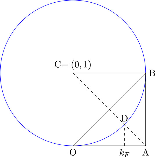
We first provide an example where the normalized k-index coincides with the Pietra index. This example is taken from Ref. 3. Let us consider an arc of a unit circle ODB as a Lorenz curve where OB is one of the diagonal (egalitarian line) of the unit square ABCO (as shown in Figure 3) where CD represents the unit radius of the circle, CA is the other diagonal of the unit square ABCO = . In this case the Lorenz curve is, where is the relevant income distribution. One can verify that . Hence, the Gini index is larger than the Pietra index and the normalized k-index. Also in this case the maximum distance between perfect equality line and the Lorenz curve is at , hence Pietra index coincides with the normalized k-index.
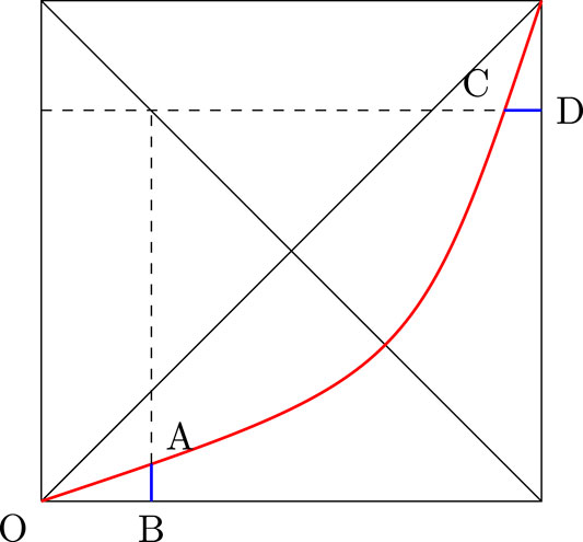
The Lorenz function is symmetric if for all , or equivalently , where . The idea of symmetry is explained in Figure 4. One can verify that the Lorenz function is symmetric. It was proved in Banerjee, Chakrabarti, Mitra, and Mutuswami [3] that, in general, if the Lorenz function is symmetric and differentiable, then the proportion associated with the Pietra index coincides with the proportion of the k-index. Hence, we also have .
The next example is one where the Pietra index coincides with the Gini index. This example is taken from Eliazar and Sokolov [18]. Fix any fraction and consider the following Lorenz function:
Figure 5 depicts this Lorenz function and in particular the curve OBA represents this Lorenz curve. One can show that . Hence, the Gini index coincides with Pietra and the normalized k-index has a lower value. Therefore, from this example we can say that k-index has different features relative to both the Gini index and the Pietra index.
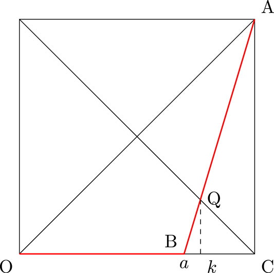
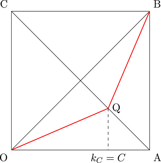
Finally, when does all the three indices coincide? It was established in Ref. 3 that all three measures will coincide if and only if the Lorenz function has the following form defined for any given :
In Figure 6, the straight lines OQ and QB taken together represents the Lorenz curve for . One can verify that
Observe that, if , then we have for all and in that case the three indices also coincide since .
It is clear that the Lorenz functions of the form with is valid for any society having two income groups. Therefore, a natural question in this context is the following: What does the coincidence of the three measures mean in terms of discrete random variables? For any discrete random variable such that , we have , with and the associated Lorenz function has the following form:
For the coincidence of all the three indices we first require that and implying that . Moreover, for the coincidence we also require , that is, which yields . Thus, from the above discussion we have the following result.
• Consider any discrete random variable discussed in Example 1 for which the Lorenz function is given by Eq. 3. The normalized k-index coincides with the Gini index and the Pietra index if and only if any one of the following conditions holds:
(C1) The society has all agents having the same income so that for all . For this case we have, .
(C2) The society has two groups of agents with one group of agents having an income of and another group of agents having an income of such that . Moreover, the Lorenz function is given in Eq. 12 with the added restrictions that , and hence . For this case we have, .
5. Ranking Lorenz Functions
Consider the uniform income distribution defined on any compact interval with . The Lorenz function is given by for all (see Figure 7). Here is the reciprocal of the Golden ratio, that is, where is the Golden ratio. Moreover, . Similarly, one can derive that the Gini index is and the Pietra index is with . Hence, we have . Similarly, consider the Pareto distribution with parameter value . The Lorenz function is given by so that and the k-index is again the reciprocal of the Golden ratio, that is, and (see Figure 7). Thus, according to the normalized k-index, a society with an income distribution is equivalent to a society with an income distribution of in terms of inequality. One can verify that this equivalence between and is also preserved under the Gini index and the Pietra index. Specifically, we have and though . Hence, we have
Consider the income distributions and defined in Example 2. From Remark 1 it follows that , from Remark 2 it follows that and from Remark 3 it also follows that . Therefore, all the three measures unambiguously assures that the society with income distribution is less unequal that the society with income distribution .
Given the above examples of this section, one may be tempted to think that ranking Lorenz functions using these three measures always gives the same order, that is, if one measure shows that the income distribution F is equivalent to another income distribution in terms of inequality, then the other two measures will also give the same result, and, if one measure shows that the income distribution F is less unequal than the income distribution , then also the other two measures will establish the same order. However, as argued in Ref. 3, this is not the case. To establish this point [3] provided the following two examples.
In the first example the following Lorenz functions were considered to establish that the normalized k-index yields a different ranking from the Pietra index.
One can show that , that is, according to the normalized k-index, the society with income distribution is equivalent to the society with income distribution in terms of inequality. However, according to the Pietra index, the society with income distribution is less unequal than the society with income distribution .
In the second example, two Lorenz functions were considered of which the first one is the standard uniform distribution defined on any compact interval of the form with , that is, for all . The other Lorenz function has the following form:
. This example demonstrates an important difference between and . The Gini index is affected by transfers within a group. In particular, the poor are unaffected but the rich (lying in the interval ) have become more egalitarian while moving from to . The normalized k-index on the other hand is unaffected with such intra-group transfers. Therefore, if we are interested in reducing inequality between groups, then the normalized k-index is a better indicator than the Gini index.
6. Numerical Observations
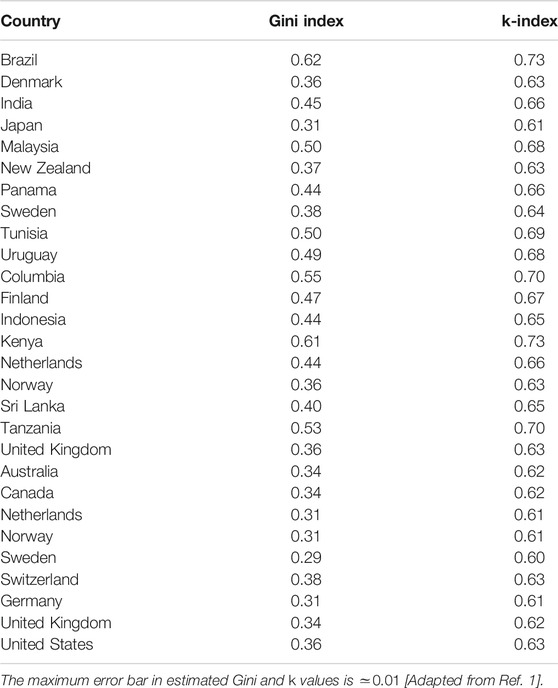
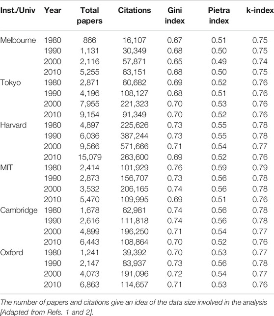
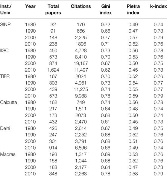
For the purpose of comparison between different inequality indices, we present in Table 1, the estimated values of the Gini and k-indices for the income distributions in some countries for the period 1963–1983. Tables 2 and 3 give the estimated values of these indices along with the Pietra index for citations, for different institutions and universities across the world observed in different years. Table 4 also shows the comparison between Gini, Pietra and k for inequalities in paper citations for various science journals. All the tables are taken from Ref. 1.
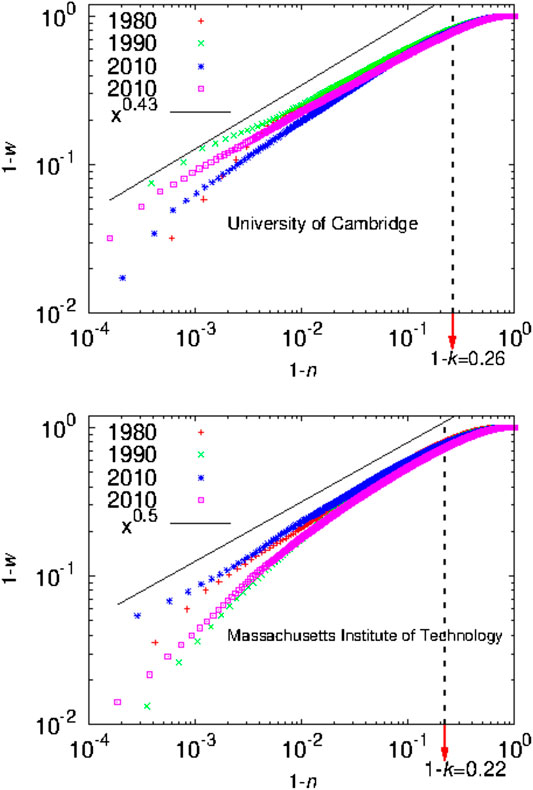
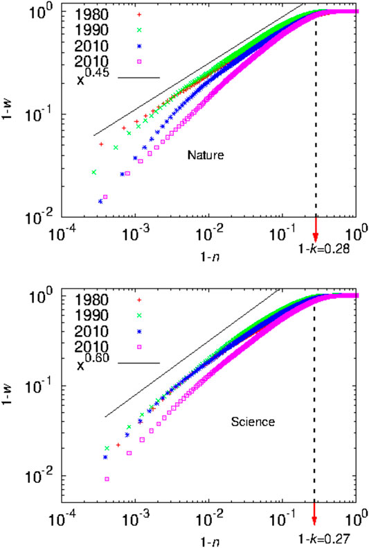
In Ref. 1 it was observed that Eq. 11 is an approximate result and can differ for large values of G and k. Furthermore, the value of k corresponds to an upper limit beyond which the distribution follows a power law pattern, similar to the celebrated Pareto law [24]. For the inequality in citation data, if n is the fraction of papers and w is the cumulative fraction of citations, then for , with which implies for and c is a proportionality constant. This is illustrated in Figures 8 and 9.
7. Summary and Discussion
For the nonlinear Lorenz function , the traditional measures like Gini index measures some “average property”, while the Kolkata index (k) identifies the non-trivial fixed point of the complementary Lorenz function ( = ; note that has trivial fixed points at and 1, while has a nontrivial fixed point at ). This k-index apart from capturing the essential character of the nonlinear Lorenz function (as inspired by the major developments of renormalization group theory in statistical physics [14] or in identifying the universal characters corresponding to the onset of chaos in nonlinear systems [15]), also gives us a very tangible one, giving that fraction of the population possess k fraction of the total wealth in the society. In Ref. 25 the k-index is used to define a generalized Gini index. In a recent study, the k-index has been used to quantify the inequality for spreading of the Covid-19 infection in urban neighbourhoods and slums in a society (see Ref. 26).
After a general introduction in Section 1, we discuss in Section 2, some structural features of the Lorenz function and introduce the Complementary Lorenz function, which has a nontrivial fixed point (namely the Kolkata index) as mentioned above. In Sections 3 and 4, we try to demonstrate the uniqueness of the k-index, compared to Gini and Pietra indices in ranking the rich-poor disparity, assuming some typical income distributions. we have argued (in Section 3) that the procedure of obtaining the h-index of any research scientist using the generated citation curve is the same as identifying the fixed point of the complementary Lorenz function of any income distribution that yields the k index. While comparing the normalized k-index with the Pietra index and with the Gini index, one can show that for any given distribution the normalized k-index is no more than the Pietra index and the Pietra index is no more than the Gini index. We have also argued (in Section 4.2) that for any given distribution the normalized k-index, the Pietra index and the Gini index coincide only if either the society is such that all agents have equal income or there are only two income groups in a society with some added restrictions (see condition C2 in this subsection). We have also argued (in Section 5) that if we are interested in reducing inequality between the rich and poor groups of the society, then the normalized k-index is a better indicator than the Gini index. In Section 6, we can see that while the Gini index value typically ranges from 0.30 to 0.62, the Kolkata index value ranges from 0.60 to 0.73 at any particular time or year for income or wealth data across the countries of the world. It may be mentioned here that income inequality data are not easily available from reliable sources. On the other hand, the (paper) citations may be considered as a measure of the wealth created by the respective University or Institution and the resulting inequality data are abundantly available in accurate digital formats (say from the ISI Web of Science). We estimated the Gini, Pietra, and Kolkata index values for the citations earned by the yearly publications of various academic institutions from such data sources. We find that while Gini and Pietra index values range from 0.65 to 0.75 and 0.50 to 0.60, respectively, the Kolkata index remains around value for Institutions or Universities across the world. As mentioned already, k-index is the social equivalent to the h-index for an individual researcher or academician. Also we find that the value for k-index gives an estimate of the crossover point beyond which the growth of income (or citations) with the fraction of population (or publications) enters a power law (Pareto) region (see Figures 8 and 9).
Author Contributions
All authors listed have made a substantial, direct, and intellectual contribution to the work and approved it for publication.
Conflict of Interest
The authors declare that the research was conducted in the absence of any commercial or financial relationships that could be construed as a potential conflict of interest.
8. Appendices
8.1. Appendix A
We formally show that for the discrete random variable with the Lorenz function is given by Eq. 3, the Gini index has the following explicit form:
Observe first that
Thus, using and using Eq. A1 we get
Hence, from the last inequality in Eq. A2 the result follows.
8.2. Appendix B
8.2.1. Appendix B (i)
The following derivation shows why this is true.
8.2.2. Appendix B (ii)
We formally show that for the discrete random variable with the Lorenz function is given by Eq. 3, the Pietra index has the following explicit form:
where is such that implying that .
For the first equality, observe that there exists such that implying that . Thus, using and using we get
Given Eq. B2 it follows that the Pietra index of the distribution with is
Given Eq. B3, we can also derive second equality by using and by using . Specifically,
Footnotes
1The end points are clear since none of the population possesses none of the income while the entire population possesses all the income.
References
1. Ghosh A, Chattopadhyay N, Chakrabarti BK. Inequality in societies, academic institutions and science journals: Gini and k-indices. Phys A (2014). 410:30–4. doi:10.1016/j.physa.2014.05.026
PubMed Abstract | CrossRef Full Text | Google Scholar
3. Banerjee S, Chakrabarti BK, Mitra M, Mutuswami S. On k-index as a measure of income inequality. Phys A (2019). 545:123178. doi:10.1016/j.physa.2019.123178
CrossRef Full Text | Google Scholar
5. Jenkins SP, Van Kerm P. The measurement of economic inequality. In: B Nolan, W Salverda, and TM Smeeding, editors The oxford handbook of economic inequality. Oxford, UK: Oxford University Press (2011).
CrossRef Full Text | Google Scholar
7. Aaberge R. Characterizations of Lorenz curves and income distributions. Soc Choice Welfare (2000). 17:639–53. doi:10.1007/s003550000046
CrossRef Full Text | Google Scholar
8. Dardanoni V, Lambert PJ. Welfare rankings of income distributions: a role for variance and some insights for tax reforms. Soc Choice Welfare (1988). 5:1–17. doi:10.1007/bf00435494
CrossRef Full Text | Google Scholar
9. Lambert PJ. The distribution and redistribution of income: a mathematical analysis. Manchester, UK: Manchester University Press (1993).
CrossRef Full Text | Google Scholar
11. Zoli C. Intersecting generalized Lorenz curves and the Gini index. Soc Choice Welfare (1999). 16:183–96. doi:10.1007/s003550050139
CrossRef Full Text | Google Scholar
14. Fisher ME. Renormalization group theory: its basis and formulation in statistical physics. Rev Mod Phys (1998). 70:653–81. doi:10.1103/revmodphys.70.653
CrossRef Full Text | Google Scholar
15. Feigenbaum MJ. Universal behavior in nonlinear systems. Phys Nonlinear Phenom (1983). 7:16–39. doi:10.1016/0167-2789(83)90112-4
CrossRef Full Text | Google Scholar
16. Gini CW. Variabilità e mutabilità: contributo allo studio delle distribuzioni e delle relazioni statistiche. Bologna, Italy: C. Cuppini (1912).
CrossRef Full Text | Google Scholar
17. Pietra G. Delle relazioni tra gli indici di variabilita. Atti del Reale Istituto Veneto di Scienze, Lettere ed Arti (1915). 74:775–804. Note I, II.
CrossRef Full Text | Google Scholar
18. Eliazar II, Sokolov IM. Measuring statistical heterogeneity: the Pietra index. Phys A (2010). 389:117–25. doi:10.1016/j.physa.2009.08.006
CrossRef Full Text | Google Scholar
22. Hirsch JE. An index to quantify an individual’s scientific research output. Proc Natl Acad Sci USA (2005). 102:16569–72. doi:10.1073/pnas.0507655102
CrossRef Full Text | Google Scholar
24. Pareto V. Cours d’économie politique. Vol. 1. Paris, France: Librairie Droz (1964).
Google Scholar
25. Subramanian S. Further tricks with the Lorenz curve. Econ Bull (2019). 39(3):1677–86.
Google Scholar
26. Sahasranaman A, Jensen HJ. Spread of Covid-19 in urban neighbourhoods and slums of the developing world. arxiv [physics.soc-ph], 2010.06958 (2020).
Google Scholar
 Suchismita Banerjee
 Bikas K. Chakrabarti
 Manipushpak Mitra
 Suresh Mutuswami