Computational Results With Non-singular and Non-local Kernel Flow of Viscous Fluid in Vertical Permeable Medium With Variant Temperature

This present article explores the transversal magnetized flow of a viscous fluid. The flow is confined to a vertical wall, saturated in permeable medium, along with ramped wall temperature. In this study, the conjugate impact of heat and mass transfer with slip and non-slip conditions are considered in the velocity field and energy equation. The dimensionless Atangana-Baleanu fractional governing equations are derived with Laplace transformation. Computational results are expressed graphically with the effect of various physical parameters. Comparative graphical analysis of the Atangana-Baleanu derivative for temperature, concentration and velocity field, with slip and non-slip impact, shows that the memory effects of the Atangana-Baleanu derivative are better than the results that exist in the literature.

1. Introduction

In nature, heat and mass transfer is a common conjugate phenomenon for chemical reaction, evaporation, and condensation caused by temperature and concentration. Consequently, the behavior of heat transfer exists in different practical applications. The heat transfer mechanism is linked with mass, to jointly produce electrically conducting fluid flow with a conjugate effect. In a preamble surface the process of thermal and mass transfer with a conjugate effect have different applications in the area of nuclear production, industry, oil production, and engineering disciplines [1, 2]. The conjugate effect with convection flow over an infinite plate in preamble medium, along time dependent velocity, electrically flow with a magnetic effect and have been studied by different researchers. Ramped wall temperatures with thermal radiation have received much interest in convection flow over boundless vertical plates [3–6]. In literature, Toki and Tokis [7] studied time dependent boundary conditions on viscous fluid over a boundless preamble plate. Senapatil et al. [8] investigated the influence of chemical parameters on viscous fluid over preamble medium with a bounded slip region. Khan et al. [9] discussed the influence of heat and mass diffusion of a viscous fluid over an oscillating plate. Das et al. [10] and Narahari and Ishaq [11] investigated the solution of unsteady Walter's fluids on convection flow over preamble medium with a magnetic effect and constant suction heat. Recently, Kumar et al. [12] discussed the fractional model for radial fins with heat transfer. Some of the latest results, according to this research, are given in Gupta et al. [13], Khan et al. [14], and Imran et al. [15].

Moreover, the application of magnetic fields is significant, with heat transfer in different situations of flow of an incompressible fluid, for example, geothermal energy, magnetic generator, and metallurgical processes. The influence of the slip and non-slip condition with the magnetic field and chemical reaction of an electrically conducting fluid over a porous surface, have been developed by Boussinesqu's approximation [16]. Jha and Apere [17] and Seth et al. [18] analyzed the ion slip and hall effect boundary conditions on a magnetized electrically conducting flow between parallel plates. The impact of the current and rotation with heat radiation and mass transfer, on time depending heat observation over a preamble surface, were taken into account. Over the last few years, fractional calculus has played a significant role in viscoelastic models. The derivative of the fractional order can be achieved by constitutive equations of well-known models through time ordinary derivatives. Recently, many fractional time derivative problems have been studied [19, 20]. Different real life problems have been investigated through fractional time operators [21–23]. A modern fractional approach has been presented without a singular kernel. A non-singular kernel is used to find the solution for MHD convection flow with ramped temperature, was investigated by Riaz et al. [24]. Furthermore, Riaz and Saeed [25] discussed the solution of MHD Oldroyd-B fluid using integer and fractional order derivatives with slip effect and time boundary conditions. The Study of natural convection flow with in channel using non-singular kernels is discussed by Saeed et al. [26].

In this paper, we discuss the computational calculation for the magnetized flow of Newtonian fluid with slip and conjugate effect, through a preamble surface. Computational results for the velocity profile, temperature gradient, and concentration field are calculated with the Atangana-Baleanu fractional derivative, through the Laplace transform. Tzou and Stehfest's algorithm is used to find the inverse Laplace transform. Further, We show the strength of non-singular and non-kernels. Fractional order Atangana-Baleanu (ABC) derivatives are used to analyze fractional parameters (memory effect) on the dynamics of fluid. We conclude that the fractional order model is best for memory effect and flow behavior of the fluid with reference to classical models. ABC is good at highlighting the dynamics of fluid. The influence of transverse magnetic fields are studied for ABC and CF. Moreover, the impact of parameters on the velocity profile are analyzed through numerical simulation and graphs for ABC and CF models. Expression from some limited and special cases were also obtained in terms of the velocity profile with different flow parameters.

2. Mathematical Model With Statement of the Problem

In this article, we assumed the slip effect between fluid and a wall. After t = 0⁺, the temperature on the plate is enhanced or reduced to ${\theta }_{\infty }+({\theta }_{\omega }-{\theta }_{\infty })\frac{t}{t_o}$ when t ≤ t_o and therefore, for t > t_o, is retained at a constant temperature θ_ω and the concentration is enhanced to C_ω. The set of governing equations are given in [27]:

$\begin{array}{ll}{v}_t=v_{\xi \xi }+G_r\theta +G_{m}C-K_{p}v-M^{2}v,& (1)\end{array}$

$\begin{array}{ll}(P_{reff}){\theta }_t={\theta }_{\xi \xi },& (2)\end{array}$

$\begin{array}{ll}{S}_c{C}_t=C_{\xi \xi }.& (3)\end{array}$

With suitable conditions

$\begin{array}{ll}v(\xi ,0)=0,\theta (\xi ,0)={\theta }_{\infty },C(\xi ,0)=C_{\infty },\forall \xi \ge 0,& (4)\end{array}$

$\begin{array}{ll}v(\xi ,t)-L(v_{\xi }{|}_{\xi =0})=\frac{f(t)}{\mu },C(0,t)=C_{\omega },t>0,& (5)\end{array}$

$\begin{array}{ll}\theta (\xi ,0)={\theta }_{\infty }+({\theta }_w-{\theta }_{\infty })\frac{t}{t_o},0<t<t_o,& (6)\end{array}$

$\begin{array}{l}v(y,t)={\theta }_{\infty },C(y,t)=C_{\infty },t>0,\\ \theta (y,t)={\theta }_{\omega },t>t_o,y\to \infty .& (7)\end{array}$

We arrive at the governing equations, in terms of the Atangana-Baleanu fractional derivative, as:

$\begin{array}{ll}{{}^{ABC}D}_t^{\alpha }v=v_{\xi \xi }+G_r\theta +G_{m}C-k_{p}v-M^{2}v,& (8)\end{array}$

$\begin{array}{ll}{{}^{ABC}D}_t^{\alpha }\theta =\left(\frac{1}{P_{reff}}\right){\theta }_{\xi \xi },& (9)\end{array}$

$\begin{array}{ll}{{}^{ABC}D}_t^{\alpha }C=\left(\frac{1}{S_c}\right)C_{\xi \xi },& (10)\end{array}$

where ${{}^{ABC}D}_t^{\alpha }$ is the fractional differential operator of order 0 < α <1 called the Atangana-Baleanu fractional operator as defined by [21, 28]:

$\begin{array}{l}{{}^{ABC}D}_t^{\alpha }f(\xi ,\tau )=\frac{M(\alpha )}{1-\alpha }{\displaystyle {\int }_0^{\tau }{E}_{\alpha }\left(-\frac{\alpha {(t-\tau )}^{\alpha }}{1-\alpha }\right)\frac{\partial f(\xi ,\tau )}{\partial \tau }d\tau },\\ with{\displaystyle \sum _{m=0}^{\infty }}\frac{{(-t)}^{\alpha m}}{\Gamma (1+\alpha m)}={\text{E}}_{\alpha }{(-t)}^{\alpha },& (11)\end{array}$

where M(α) denotes a normalization function obeying M(0) = M(1) = 1.

The Laplace transform of Equation (11) is as follows [26]:

$\begin{array}{ll}L\left[{{}^{ABC}D}_t^{\alpha }f(\xi ,\tau )\right]=\frac{s^{\alpha }L[f(\xi ,\tau )]-s^{\alpha -1}f(\xi ,0)}{(1-\alpha )s^{\alpha }+\alpha }.& (12)\end{array}$

The appropriate initial and boundary conditions are:

$\begin{array}{ll}v(\xi ,0)=\theta (\xi ,0)=C(\xi ,0)=0,\forall \xi \ge 0,& (13)\end{array}$

$\begin{array}{ll}v(\xi ,t)-h{v}_{\xi }{|}_{\xi =0}=Z(t),& (14)\end{array}$

$\begin{array}{ll}C(0,t)=1,C(\infty ,t)=0,t>0,& (15)\end{array}$

$\begin{array}{ll}\theta (\infty ,t)=0,v(\infty ,t)=0,t>0,& (16)\end{array}$

$\begin{array}{ll}\theta (0,t)=t,0<t\le 1,\theta (0,t)=1,t>1.& (17)\end{array}$

3. Solution of the Problem

3.1. Distribution of Temperature Gradient With Fractional Model 0 < α <1

In order to find the solution of fractional concentration distribution, we employ Equation (12) into Equation (9), and obtain:

$\begin{array}{ll}\left(\frac{s^{\alpha }}{(1-\alpha )s^{\alpha }+\alpha }\right)\bar{\theta }(\xi ,s)=\frac{1}{P_{reff}}\overline{{\theta }_{\xi \xi }}(\xi ,s),& (18)\end{array}$

$\begin{array}{ll}\bar{\theta }(\xi ,s)=c_1{e}^{-\xi \sqrt{P_{reff}\left(\frac{s^{\alpha }}{(1-\alpha )s^{\alpha }+\alpha }\right)}}+c_2{e}^{\xi \sqrt{P_{reff}\left(\frac{s^{\alpha }}{(1-\alpha )s^{\alpha }+\alpha }\right)}},& (19)\end{array}$

with the help of (13)–(17), we find the values of constants c₁ and c₂, and we have.

$\begin{array}{ll}\bar{\theta }(\xi ,s)=\left(\frac{1-e^{-s}}{s^2}\right)e^{-\xi \sqrt{P_{reff}\left(\frac{s^{\alpha }}{(1-\alpha )s^{\alpha }+\alpha }\right)}}.& (20)\end{array}$

3.2. Distribution of Concentration Gradient With Fractional Model 0 < α <1

In order to find the solution of fractional concentration distribution, we employ Equation (12) into Equation (10), and obtain:

$\begin{array}{ll}\left(\frac{s^{\alpha }}{(1-\alpha )s^{\alpha }+\alpha }\right)\bar{C}(\xi ,s)=\frac{1}{S_c}\overline{C_{\xi \xi }}(\xi ,s),& (21)\end{array}$

$\begin{array}{ll}\bar{C}(\xi ,s)=c_1{e}^{-\xi \sqrt{S_c\left(\frac{s^{\alpha }}{(1-\alpha )s^{\alpha }+\alpha }\right)}}+c_2{e}^{\xi \sqrt{S_c\left(\frac{s^{\alpha }}{(1-\alpha )s^{\alpha }+\alpha }\right)}},& (22)\end{array}$

with the help of (13)–(17), we find the values of constants c₁ and c₂, and we have.

$\begin{array}{ll}\bar{C}(\xi ,s)=\left(\frac{1}{s}\right)e^{-\xi \sqrt{S_c\left(\frac{s^{\alpha }}{(1-\alpha )s^{\alpha }+\alpha }\right)}}.& (23)\end{array}$

3.3. Distribution of Velocity Field With Fractional Model 0 < α <1

In order to find the solution of the fractional concentration distribution, we employ Equation (12) into Equation (8), and obtain:

$\begin{array}{l}(\frac{s^{\alpha }}{(1-\alpha )s^{\alpha }+\alpha })\bar{v}(\xi ,s)=v_{\xi \xi }+G_r\bar{\theta }(\xi ,s)+G_m\bar{C}(\xi ,s)\\ -k_p\bar{v}(\xi ,s)-M^2\bar{v}(\xi ,s).& (24)\end{array}$

The solution of the homogeneous part of the second order partial differential equation say that (24) is,

$\begin{array}{ll}\overline{v}(\xi ,s)=c_1{e}^{-\xi \sqrt{\left(\frac{s^{\alpha }}{(1-\alpha )s^{\alpha }+\alpha }\right)+k_p+M^2}}+c_2{e}^{\xi \sqrt{\left(\frac{s^{\alpha }}{(1-\alpha )s^{\alpha }+\alpha }\right)+k_p+M^2}}.& (25)\end{array}$

The general solution can be give as follows, after making use of $\bar{\theta }(\xi ,s)$ and $\bar{C}(\xi ,s)$,

$\begin{array}{l}\overline{v}(\xi ,s)=c_1{e}^{-\xi \sqrt{\left(\frac{s^{\alpha }}{(1-\alpha )s^{\alpha }+\alpha }\right)+k_p+M^2}}+c_2{e}^{\xi \sqrt{\left(\frac{s^{\alpha }}{(1-\alpha )s^{\alpha }+\alpha }\right)+k_p+M^2}}\\ -\frac{G_r(1-e^{-s})\left((1-\alpha )s^{\alpha }+\alpha \right)}{s^2\left(\frac{s^{\alpha }}{(1-\alpha )s^{\alpha }+\alpha }(P_{reff}-1)-(k_p+M^2)\right)}{e}^{-\xi \sqrt{P_{reff}\left(\frac{s^{\alpha }}{(1-\alpha )s^{\alpha }+\alpha }\right)}}\\ -\frac{G_3\left((1-\alpha )s^{\alpha }+\alpha \right)}{s\left(\frac{s^{\alpha }}{(1-\alpha )s^{\alpha }+\alpha }(S_c-1)-(k_p+M^2)\right)}{e}^{-\xi \sqrt{S_c\left(\frac{s^{\alpha }}{(1-\alpha )s^{\alpha }+\alpha }\right)}},& (26)\end{array}$

with the help of Equations (13)–(17), we find the values of constants c₁ and c₂ for the velocity equation:

$\begin{array}{l}\overline{v}(\xi ,s)=[\frac{1}{1+h\sqrt{\frac{s^{\alpha }}{(1-\alpha )s^{\alpha }+\alpha }}+k_p+M^2}\\ \{\frac{G_r(1-e^{-s})}{s^2}\left(\frac{1+h\sqrt{s^{\alpha }{P}_{reff}}}{\frac{s^{\alpha }}{(1-\alpha )s^{\alpha }+\alpha }(P_{reff}-1)-(k_p+M^2)}\right)\\ +\frac{G_m}{s}\left(\frac{1+h\sqrt{s^{\alpha }{S}_c}}{\frac{s^{\alpha }}{(1-\alpha )s^{\alpha }+\alpha }(S_c-1)-(k_p+M^2)}\right)+Z(s)\}]\\ \left(e^{-\xi \sqrt{\frac{s^{\alpha }}{(1-\alpha )s^{\alpha }+\alpha }+k_p+M^2}}\right)\\ -\frac{G_r(1-e^{-s})}{s^2}\left(\frac{e^{-\xi \sqrt{s^{\alpha }{P}_{reff}}}}{\frac{s^{\alpha }}{(1-\alpha )s^{\alpha }+\alpha }(P_{reff}-1)-(k_p+M^2)}\right)\\ -\frac{G_m}{s}\left(\frac{e^{-\xi \sqrt{s^{\alpha }{S}_c}}}{\frac{s^{\alpha }}{(1-\alpha )s^{\alpha }+\alpha }(S_c-1)-(k_p+M^2)}\right).& (27)\end{array}$

The skin friction is defined as:

$\begin{array}{ll}\overline{\tau }(\xi ,s)=-\frac{\partial \overline{v}(\xi ,s)}{\partial \xi }{|}_{\xi =0},& (28)\end{array}$

$\begin{array}{l}\overline{\tau }(\xi ,s)=[\frac{1}{1+h\sqrt{\frac{s^{\alpha }}{(1-\alpha )s^{\alpha }+\alpha }}+k_p+M^2}\\ \{\frac{G_r(1-e^{-s})}{s^2}\left(\frac{1+h\sqrt{s^{\alpha }{P}_{reff}}}{\frac{s^{\alpha }}{(1-\alpha )s^{\alpha }+\alpha }(P_{reff}-1)-(k_p+M^2)}\right)\\ +\frac{G_m}{s}\left(\frac{1+h\sqrt{s^{\alpha }{S}_c}}{\frac{s^{\alpha }}{(1-\alpha )s^{\alpha }+\alpha }(S_c-1)-(k_p+M^2)}\right)+Z(s)\}]\\ \left(\sqrt{\frac{s^{\alpha }}{(1-\alpha )s^{\alpha }+\alpha }+k_p+M^2}\right)\\ -\frac{G_r(1-e^{-s})}{s^2}\left(\frac{\sqrt{s^{\alpha }{P}_{reff}}}{\frac{s^{\alpha }}{(1-\alpha )s^{\alpha }+\alpha }(P_{reff}-1)-(k_p+M^2)}\right)\\ -\frac{G_m}{s}\left(\frac{\sqrt{s^{\alpha }{S}_c}}{\frac{s^{\alpha }}{(1-\alpha )s^{\alpha }+\alpha }(S_c-1)-(k_p+M^2)}\right).& (29)\end{array}$

4. Limiting Cases

A comparative study of the existing literature and the Atangana-Baleanu derivative for some limiting cases are recovered from the general solution of (Equation 30, [27]) and the general solution of the given problem at Equation (27), are both discussed in this section.

4.1. Results With Ramped Wall Temperature and Without Porosity Effect (k_p → 0)

The velocity profile with the Atangana-Baleanu derivative is expressed for a general solution of the given problem at Equation (27) is given as:

$\begin{array}{l}\overline{v}(\xi ,s)=[\frac{1}{1+h\sqrt{\frac{s^{\alpha }}{(1-\alpha )s^{\alpha }+\alpha }}+M^2}\\ \{\frac{G_r(1-e^{-s})}{s^2}\left(\frac{1+h\sqrt{s^{\alpha }{P}_{reff}}}{\frac{s^{\alpha }}{(1-\alpha )s^{\alpha }+\alpha }(P_{reff}-1)-M^2}\right)\\ +\frac{G_m}{s}\left(\frac{1+h\sqrt{s^{\alpha }{S}_c}}{\frac{s^{\alpha }}{(1-\alpha )s^{\alpha }+\alpha }(S_c-1)-M^2}\right)+Z(s)\}]\\ \left(e^{-\xi \sqrt{\frac{s^{\alpha }}{(1-\alpha )s^{\alpha }+\alpha }+M^2}}\right)-\frac{G_r(1-e^{-s})}{s^2}\\ \left(\frac{e^{-\xi \sqrt{s^{\alpha }{P}_{reff}}}}{\frac{s^{\alpha }}{(1-\alpha )s^{\alpha }+\alpha }(P_{reff}-1)-M^2}\right)\\ -\frac{G_m}{s}\left(\frac{e^{-\xi \sqrt{s^{\alpha }{S}_c}}}{\frac{s^{\alpha }}{(1-\alpha )s^{\alpha }+\alpha }(S_c-1)-M^2}\right).& (30)\end{array}$

4.2. Results Without Thermal Radiation (N_r → 0)

The velocity profile is obtained with the Atangana-Baleanu derivative for the general solution of the given problem at Equation (27) is given as:

$\begin{array}{l}\overline{v}(\xi ,s)=[\frac{1}{1+h\sqrt{\frac{s^{\alpha }}{(1-\alpha )s^{\alpha }+\alpha }}+k_p+M^2}\\ \{\frac{G_r(1-e^{-s})}{s^2}\left(\frac{1+h\sqrt{s^{\alpha }{P}_r}}{\frac{s^{\alpha }}{(1-\alpha )s^{\alpha }+\alpha }(P_r-1)-(k_p+M^2)}\right)\\ +\frac{G_m}{s}\left(\frac{1+h\sqrt{s^{\alpha }{S}_c}}{\frac{s^{\alpha }}{(1-\alpha )s^{\alpha }+\alpha }(S_c-1)-(k_p+M^2)}\right)+Z(s)\}]\\ \left(e^{-\xi \sqrt{\frac{s^{\alpha }}{(1-\alpha )s^{\alpha }+\alpha }+k_p+M^2}}\right)\\ -\frac{G_r(1-e^{-s})}{s^2}\left(\frac{e^{-\xi \sqrt{s^{\alpha }{P}_r}}}{\frac{s^{\alpha }}{(1-\alpha )s^{\alpha }+\alpha }(P_r-1)-(k_p+M^2)}\right)\\ -\frac{G_m}{s}\left(\frac{e^{-\xi \sqrt{s^{\alpha }{S}_c}}}{\frac{s^{\alpha }}{(1-\alpha )s^{\alpha }+\alpha }(S_c-1)-(k_p+M^2)}\right).& (31)\end{array}$

4.3. Result Without Magnetic Parameter (M → 0)

The velocity profile is obtained with the Atangana-Baleanu derivative for the general solution of the given problem at Equation (27) is given as:

$\begin{array}{l}\overline{v}(\xi ,s)=[\frac{1}{1+h\sqrt{\frac{s^{\alpha }}{(1-\alpha )s^{\alpha }+\alpha }}+k_p}\\ \{\frac{G_r(1-e^{-s})}{s^2}\left(\frac{1+h\sqrt{s^{\alpha }{P}_{reff}}}{\frac{s^{\alpha }}{(1-\alpha )s^{\alpha }+\alpha }(P_{reff}-1)-k_p}\right)+\frac{G_m}{s}\\ \left(\frac{1+h\sqrt{s^{\alpha }{S}_c}}{\frac{s^{\alpha }}{(1-\alpha )s^{\alpha }+\alpha }(S_c-1)-k_p}\right)+Z(s)\}]\left(e^{-\xi \sqrt{\frac{s^{\alpha }}{(1-\alpha )s^{\alpha }+\alpha }+k_p}}\right)\\ -\frac{G_r(1-e^{-s})}{s^2}\left(\frac{e^{-\xi \sqrt{s^{\alpha }{P}_{reff}}}}{\frac{s^{\alpha }}{(1-\alpha )s^{\alpha }+\alpha }(P_{reff}-1)-k_p}\right)\\ -\frac{G_m}{s}\left(\frac{e^{-\xi \sqrt{s^{\alpha }{S}_c}}}{\frac{s^{\alpha }}{(1-\alpha )s^{\alpha }+\alpha }(S_c-1)-k_p}\right).& (32)\end{array}$

5. Special Cases

For validation and to check our general results in this section, we will discuss some special cases by customizing the value of f(t). Moreover, our aim is to provide a comparison of our results with the Caputo-Fabrizio (CF) time fractional derivative.

5.1. Case-I

By putting z(t) = t into Equation (27), we obtain a suitable result for the velocity profile:

$\begin{array}{l}\overline{v}(\xi ,s)=[\frac{1}{1+h\sqrt{\frac{s^{\alpha }}{(1-\alpha )s^{\alpha }+\alpha }}+k_p+M^2}\\ \{\frac{G_r(1-e^{-s})}{s^2}\left(\frac{1+h\sqrt{s^{\alpha }{P}_{reff}}}{\frac{s^{\alpha }}{(1-\alpha )s^{\alpha }+\alpha }(P_{reff}-1)-(k_p+M^2)}\right)\\ +\frac{G_m}{s}\left(\frac{1+h\sqrt{s^{\alpha }{S}_c}}{\frac{s^{\alpha }}{(1-\alpha )s^{\alpha }+\alpha }(S_c-1)-(k_p+M^2)}\right)+\frac{1}{s^2}\}]\\ \left(e^{-\xi \sqrt{\frac{s^{\alpha }}{(1-\alpha )s^{\alpha }+\alpha }+k_p+M^2}}\right)\\ -\frac{G_r(1-e^{-s})}{s^2}\left(\frac{e^{-\xi \sqrt{s^{\alpha }{P}_{reff}}}}{\frac{s^{\alpha }}{(1-\alpha )s^{\alpha }+\alpha }(P_{reff}-1)-(k_p+M^2)}\right)\\ -\frac{G_m}{s}\left(\frac{e^{-\xi \sqrt{s^{\alpha }{S}_c}}}{\frac{s^{\alpha }}{(1-\alpha )s^{\alpha }+\alpha }(S_c-1)-(k_p+M^2)}\right).& (33)\end{array}$

The analogs of the velocity profile are obtained by (Equation 40, [27]) using the CF operator:

$\begin{array}{l}\overline{v}(\xi ,s)=[\frac{1}{1+h\sqrt{\frac{s}{(1-\alpha )s+\alpha }}+k_p+M^2}\\ \{\frac{G_r(1-e^{-s})}{s^2}\left(\frac{1+h\sqrt{s{P}_{reff}}}{s{P}_{reff}-\frac{s}{(1-\alpha )s+\alpha }-(k_p+M^2)}\right)\\ +\frac{G_m}{s}\left(\frac{1+h\sqrt{s{S}_c}}{s{S}_c-\frac{s}{(1-\alpha )s+\alpha }-(k_p+M^2)}\right)+\frac{1}{s^2}\}]\\ \left(e^{-\xi \sqrt{\frac{s}{(1-\alpha )s+\alpha }+k_p+M^2}}\right)\\ -\frac{G_r(1-e^{-s})}{s^2}\left(\frac{e^{-\xi \sqrt{s{P}_{reff}}}}{s{P}_{reff}-\frac{s}{(1-\alpha )s+\alpha }-(k_p+M^2)}\right)\\ -\frac{G_m}{s}\left(\frac{e^{-\xi \sqrt{s{S}_c}}}{s{S}_c-\frac{s}{(1-\alpha )s+\alpha }-(k_p+M^2)}\right).& (34)\end{array}$

Graphs for the profiles of the velocity for both operators for the variation of physical parameters α, P_reff, M, G_r, G_m, S_c, and k_p are prepared. Moreover, the slip and no slip effects are significant. It is noted that the memory effects obtained by the Atangana-Baleanu derivative express more significant results than the results recovered by the Caputo-Fabrizio derivative.

5.2. Case-II

By putting z(t) = te^t into Equation (27), we obtain a suitable result for the velocity profile:

$\begin{array}{l}\overline{v}(\xi ,s)=[\frac{1}{1+h\sqrt{\frac{s^{\alpha }}{(1-\alpha )s^{\alpha }+\alpha }}+k_p+M^2}\\ \{\frac{G_r(1-e^{-s})}{s^2}\left(\frac{1+h\sqrt{s^{\alpha }{P}_{reff}}}{\frac{s^{\alpha }}{(1-\alpha )s^{\alpha }+\alpha }(P_{reff}-1)-(k_p+M^2)}\right)\\ +\frac{G_m}{s}\left(\frac{1+h\sqrt{s^{\alpha }{S}_c}}{\frac{s^{\alpha }}{(1-\alpha )s^{\alpha }+\alpha }(S_c-1)-(k_p+M^2)}\right)+\frac{1}{{(s-1)}^2}\}]\\ \left(e^{-\xi \sqrt{\frac{s^{\alpha }}{(1-\alpha )s^{\alpha }+\alpha }+k_p+M^2}}\right)\\ -\frac{G_r(1-e^{-s})}{s^2}\left(\frac{e^{-\xi \sqrt{s^{\alpha }{P}_{reff}}}}{\frac{s^{\alpha }}{(1-\alpha )s^{\alpha }+\alpha }(P_{reff}-1)-(k_p+M^2)}\right)\\ -\frac{G_m}{s}\left(\frac{e^{-\xi \sqrt{s^{\alpha }{S}_c}}}{\frac{s^{\alpha }}{(1-\alpha )s^{\alpha }+\alpha }(S_c-1)-(k_p+M^2)}\right).& (35)\end{array}$

The analogs of the velocity profile are obtained by (Equation 42, [27]) using CF operator:

$\begin{array}{l}\overline{v}(\xi ,s)=[\frac{1}{1+h\sqrt{\frac{s}{(1-\alpha )s+\alpha }}+k_p+M^2}\\ \{\frac{G_r(1-e^{-s})}{s^2}\left(\frac{1+h\sqrt{s{P}_{reff}}}{s{P}_{reff}-\frac{s}{(1-\alpha )s+\alpha }-(k_p+M^2)}\right)\\ +\frac{G_m}{s}\left(\frac{1+h\sqrt{s{S}_c}}{s{S}_c-\frac{s}{(1-\alpha )s+\alpha }-(k_p+M^2)}\right)+\frac{1}{{(s-1)}^2}\}]\\ \left(e^{-\xi \sqrt{\frac{s}{(1-\alpha )s+\alpha }+k_p+M^2}}\right)\\ -\frac{G_r(1-e^{-s})}{s^2}\left(\frac{e^{-\xi \sqrt{s{P}_{reff}}}}{s{P}_{reff}-\frac{s}{(1-\alpha )s+\alpha }-(k_p+M^2)}\right)\\ -\frac{G_m}{s}\left(\frac{e^{-\xi \sqrt{s{S}_c}}}{s{S}_c-\frac{s}{(1-\alpha )s+\alpha }-(k_p+M^2)}\right).& (36)\end{array}$

5.3. Case-III

By putting z(t) = sin(ωt) into Equation (27), we obtain a suitable result for the velocity profile:

$\begin{array}{l}\overline{v}(\xi ,s)=[\frac{1}{1+h\sqrt{\frac{s^{\alpha }}{(1-\alpha )s^{\alpha }+\alpha }}+k_p+M^2}\\ \{\frac{G_r(1-e^{-s})}{s^2}\left(\frac{1+h\sqrt{s^{\alpha }{P}_{reff}}}{\frac{s^{\alpha }}{(1-\alpha )s^{\alpha }+\alpha }(P_{reff}-1)-(k_p+M^2)}\right)\\ +\frac{G_m}{s}\left(\frac{1+h\sqrt{s^{\alpha }{S}_c}}{\frac{s^{\alpha }}{(1-\alpha )s^{\alpha }+\alpha }(S_c-1)-(k_p+M^2)}\right)+\frac{\omega }{s^2+{\omega }^2}\}]\\ \left(e^{-\xi \sqrt{\frac{s^{\alpha }}{(1-\alpha )s^{\alpha }+\alpha }+k_p+M^2}}\right)-\frac{G_r(1-e^{-s})}{s^2}\\ \left(\frac{e^{-\xi \sqrt{s^{\alpha }{P}_{reff}}}}{\frac{s^{\alpha }}{(1-\alpha )s^{\alpha }+\alpha }(P_{reff}-1)-(k_p+M^2)}\right)\\ -\frac{G_m}{s}\left(\frac{e^{-\xi \sqrt{s^{\alpha }{S}_c}}}{\frac{s^{\alpha }}{(1-\alpha )s^{\alpha }+\alpha }(S_c-1)-(k_p+M^2)}\right).& (37)\end{array}$

The analogs of the velocity profile are obtained by (Equation 44, [27]) using CF operator:

$\begin{array}{l}\overline{v}(\xi ,s)=[\frac{1}{1+h\sqrt{\frac{s}{(1-\alpha )s+\alpha }}+k_p+M^2}\\ \{\frac{G_r(1-e^{-s})}{s^2}\left(\frac{1+h\sqrt{s{P}_{reff}}}{s{P}_{reff}-\frac{s}{(1-\alpha )s+\alpha }-(k_p+M^2)}\right)\\ +\frac{G_m}{s}\left(\frac{1+h\sqrt{s{S}_c}}{s{S}_c-\frac{s}{(1-\alpha )s+\alpha }-(k_p+M^2)}\right)+\frac{\omega }{s^2+{\omega }^2}\}]\\ \left(e^{-\xi \sqrt{\frac{s}{(1-\alpha )s+\alpha }+k_p+M^2}}\right)\\ -\frac{G_r(1-e^{-s})}{s^2}\left(\frac{e^{-\xi \sqrt{s{P}_{reff}}}}{s{P}_{reff}-\frac{s}{(1-\alpha )s+\alpha }-(k_p+M^2)}\right)\\ -\frac{G_m}{s}\left(\frac{e^{-\xi \sqrt{s{S}_c}}}{s{S}_c-\frac{s}{(1-\alpha )s+\alpha }-(k_p+M^2)}\right).& (38)\end{array}$

5.4. Case-IV

By putting z(t) = tsin(ωt) into Equation (27), we obtain a suitable result for the velocity profile:

$\begin{array}{l}\overline{v}(\xi ,s)=[\frac{1}{1+h\sqrt{\frac{s^{\alpha }}{(1-\alpha )s^{\alpha }+\alpha }}+k_p+M^2}\\ \{\frac{G_r(1-e^{-s})}{s^2}\left(\frac{1+h\sqrt{s^{\alpha }{P}_{reff}}}{\frac{s^{\alpha }}{(1-\alpha )s^{\alpha }+\alpha }(P_{reff}-1)-(k_p+M^2)}\right)\\ +\frac{G_m}{s}\left(\frac{1+h\sqrt{s^{\alpha }{S}_c}}{\frac{s^{\alpha }}{(1-\alpha )s^{\alpha }+\alpha }(S_c-1)-(k_p+M^2)}\right)+\frac{2s\omega }{s^2+{\omega }^2}\}]\\ \left(e^{-\xi \sqrt{\frac{s^{\alpha }}{(1-\alpha )s^{\alpha }+\alpha }+k_p+M^2}}\right)\\ -\frac{G_r(1-e^{-s})}{s^2}\left(\frac{e^{-\xi \sqrt{s^{\alpha }{P}_{reff}}}}{\frac{s^{\alpha }}{(1-\alpha )s^{\alpha }+\alpha }(P_{reff}-1)-(k_p+M^2)}\right)\\ -\frac{G_m}{s}\left(\frac{e^{-\xi \sqrt{s^{\alpha }{S}_c}}}{\frac{s^{\alpha }}{(1-\alpha )s^{\alpha }+\alpha }(S_c-1)-(k_p+M^2)}\right).& (39)\end{array}$

The analogs of the velocity profile are obtained by (Equation 46, [27]) using CF operator:

$\begin{array}{l}\overline{v}(\xi ,s)=[\frac{1}{1+h\sqrt{\frac{s}{(1-\alpha )s+\alpha }}+k_p+M^2}\\ \{\frac{G_r(1-e^{-s})}{s^2}\left(\frac{1+h\sqrt{s{P}_{reff}}}{s{P}_{reff}-\frac{s}{(1-\alpha )s+\alpha }-(k_p+M^2)}\right)\\ +\frac{G_m}{s}\left(\frac{1+h\sqrt{s{S}_c}}{s{S}_c-\frac{s}{(1-\alpha )s+\alpha }-(k_p+M^2)}\right)+\frac{2s\omega }{s^2+{\omega }^2}\}]\\ \left(e^{-\xi \sqrt{\frac{s}{(1-\alpha )s+\alpha }+k_p+M^2}}\right)\\ -\frac{G_r(1-e^{-s})}{s^2}\left(\frac{e^{-\xi \sqrt{s{P}_{reff}}}}{s{P}_{reff}-\frac{s}{(1-\alpha )s+\alpha }-(k_p+M^2)}\right)\\ -\frac{G_m}{s}\left(\frac{e^{-\xi \sqrt{s{S}_c}}}{s{S}_c-\frac{s}{(1-\alpha )s+\alpha }-(k_p+M^2)}\right).& (40)\end{array}$

By making α → 1 in Equations (20), (23), and (27) we obtain a result for a classical model, the same as that discussed by Ghalib et al. [27]. This validates our obtained results. In our flow models, we use the Laplace transform technique to solve this model, using the definition of the ABC model. In order to find the inverse, we use Stehfest's algorithms [29] for semi-analytical solutions. Stehfest's algorithms are used for the verification of our inverse Laplace transformation

$\begin{array}{l}v(y,t)=\frac{ln(2)}{t}{\displaystyle \sum _{j=1}^{2m}{d}_j}\overline{v}(y,j\frac{ln(2)}{t}),\\ d_j={(-1)}^{j+m}{\displaystyle \sum _{i=[\frac{j+1}{2}]}^{min(j,m)}\frac{i^m(2i)!}{(m-i)!i!(i-1)!(j-i)!(2i-j)!}}.\end{array}$

6. Results and Discussion

The physical aspects of the CF and ABC time derivative are discussed in the given problem. Numerical results for T, C, and v are plotted using MATHCAD for embedded physical parameters, such as M, k_p, P_reff, G_r, G_m, S_c, and slip parameter h. Figure 1 shows the behavior of α on temperature. It is shown that the value of α increases, while the temperature of the fluid decreases. The memory effect is explained well with the ABC derivative in comparison to the CF derivative.

FIGURE 1

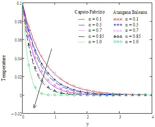
Figure 1. Variations in temperature with altered values of α and other parameters are k_p = 1.5, G_r = 2, P_reff = 0.1, G_m = 0.75, M = 0.9, and S_c = 0.5.

Figure 2 examines the behavior of α on concentration. It reduces as the value of α increases. The Antangna-Baleanu derivative shows significant behavior in comparison to the Caputo-Febrizio derivative for different values of α. Graphs for the velocity, with function f(t) = t, are shown in Figures 3–9, and with function f(t) = sin(ωt), as shown in Figures 10–16. Fluid velocity decreases with the increase of α as well as for slip and non-slip boundary conditions. Figure 3 shows that the memory effects of the Antangna Baleanu derivatives, with short and long time for the velocity profile, as well as with slip and non-slip conditions, are more significant than the memory effects of the Caputo Febrizio derivatives. For longer times, the graphical representation of the velocity shows inverse behavior, as the velocity increases with the increase of the value of α, for both the velocity profile and slip and non-slip velocity. Variation in fluid velocity with respect to the porosity coefficient is displayed in Figures 4, 11. It represents the increase in the porosity coefficient, resulting in the decrease in the velocity profile, as well as the velocity with slip and non-slip boundary conditions for both a short and long time. The representation of the velocity profile with the Antangna Baleanu derivatives, for a short and long time, as well as fluid velocity with the slip and non-slip effect is more significant than the velocities recovered with the Caputo-Fabrizio derivatives. Figures 5, 12 illustrate the influence of the Grashof number G_r on the fluid velocity, which increases with the increase of the Grashof number G_r for a short time as well as for a long time, both in the case of the slip and non-slip effects, because the thermal buoyancy forces tend to accelerate the fluid velocity for different times. The memory effects of the Antangna Baleanu derivatives for the variation of G_r with a short time and long time, oncovers more significant memory effects than the Caputo Febrizio derivatives. The velocity profile for different values of the effective Prandtl number P_reff are shown in Figures 6, 13. Fluid velocity decreases with the increase of P_reff for different times, also in the case of slip and non-slip boundary conditions. Graphical representation for various values of P_reff with the Antangna-Baleanu derivative is more impressive for short and long times as well as for slip and non-slip boundary conditions, than it is for the caputo-Fabrizio derivatives. Figures 7, 14 display the influence of the variation of a modified Grashof number G_m, and the fluid velocity increases with the increase of G_m for various times, as well as with the slip and non-slip parameters. Memory effects with the Antangna-Baleanu derivatives are better than with the Caputo-Fabrizio derivatives. The velocity profile for different values of magnetic field M are given in Figures 8, 15. Fluid velocity shrinks on a large value of M with a short time as well as with long time. It also displays the same behavior for both slip and non-slip boundary conditions, particularly, on increasing the value of M causes to enhance the frictional force which tends to resist the flow of fluid and, thus, velocity ultimately decreases. Moreover, we observed that the fluid velocity obtained with the Atangana-Baleanu derivatives for the variation of M, in case of both a short and long time, is more significant than the velocity obtained with the Caputo-Fabrizio derivatives. In Figures 9, 16 velocity profiles with variations of S_c are shown. It was found that the velocity decreases when increasing the value of S_c for both short and long times, as well as for slip and non-slip parameters. The velocity profile of different values of S_c with the Atangana-Baleanu derivatives for various times, are more expressive than the velocity that is obtained with the Caputo-Fabrizio derivatives. In Figure 10 fluid velocity reduces with enlarged values of α. It also shows the same behavior with slip as well as non-slip fluid flow conditions, and it shows the same behavior for short and long times. Memory effects show better results with the Atangana-Baleanu derivative in comparison to the Caputo-Fabrizio derivative.

FIGURE 2

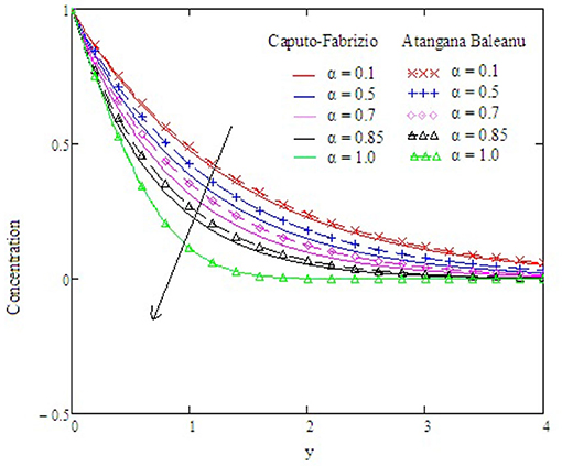
Figure 2. Variations in concentration with altered values of α and other parameters are k_p = 1.5, G_r = 2, P_reff = 0.1, G_m = 0.75, and M = 0.9.

FIGURE 3

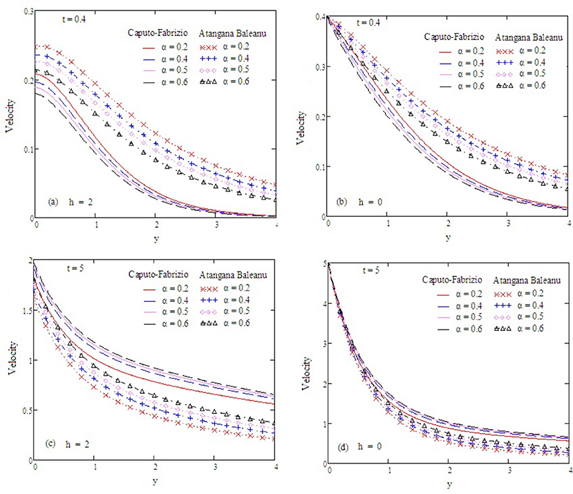
Figure 3. Velocity profiles with altered values of α and other parameters are k_p = 1.5, G_r = 2, P_reff = 0.1, G_m = 0.75, M = 0.9, and S_c = 0.5.

FIGURE 4

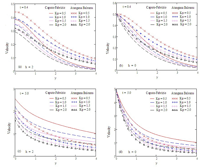
Figure 4. Velocity profiles with altered values of k_p and other parameters are G_r = 2, α = 0.5, P_reff = 0.1, G_m = 0.75, M = 0.9, and S_c = 0.5.

FIGURE 5

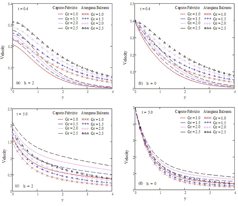
Figure 5. Velocity profiles with altered values of G_r and other parameters are k_p = 1.5, G_m = 0.75, P_reff = 0.1, α = 0.5, M = 0.9, and S_c = 0.5 G_r = 2.

FIGURE 6

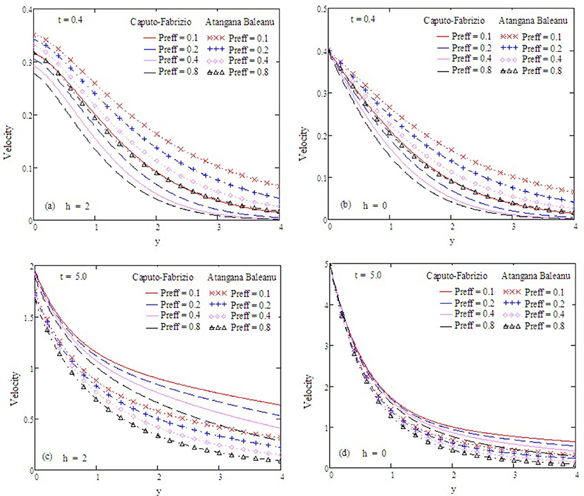
Figure 6. Velocity profiles with altered values of P_reff and other parameters are α = 0.5, G_r = 2, M = 0.9, G_m = 0.75, k_p = 1.5, and S_c = 0.5.

FIGURE 7

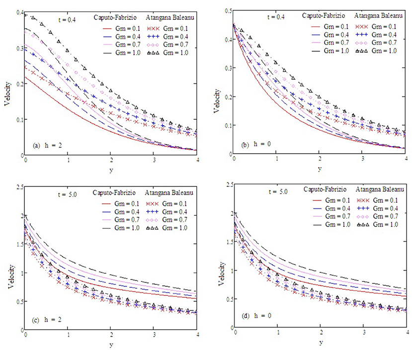
Figure 7. Velocity profiles with altered values of G_m and other parameters are α = 0.5, G_r = 2, P_reff = 0.1, k_p = 1.5, M = 0.9, and S_c = 0.5.

FIGURE 8

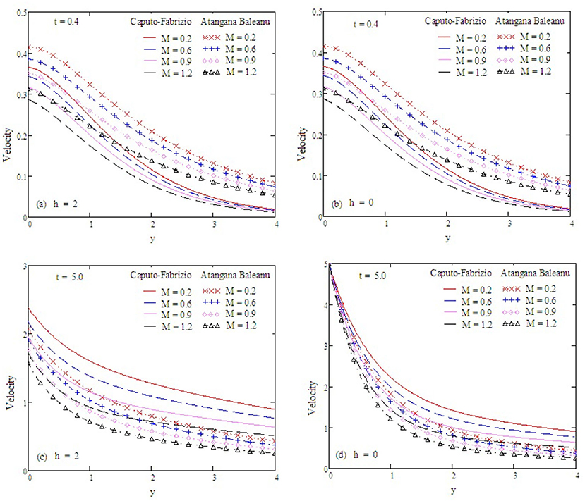
Figure 8. Velocity profiles with altered values of M and other parameters are α = 0.5, G_r = 2, P_reff = 0.1, G_m = 0.75, k_p = 1.5, and S_c = 0.5.

FIGURE 9

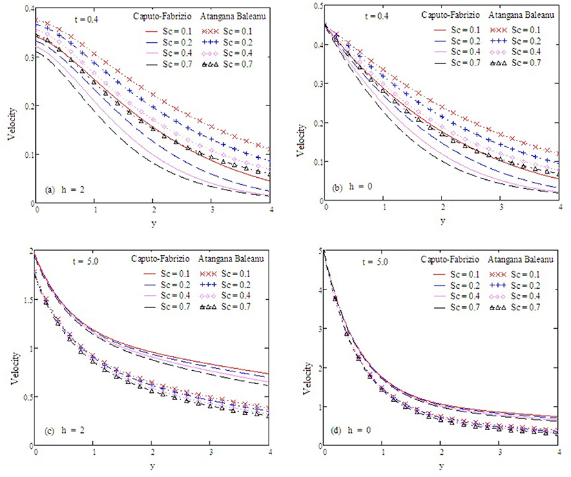
Figure 9. Velocity profiles with altered values of S_c and other parameters are α = 0.5, G_r = 2, P_reff = 0.1, G_m = 0.75, k_p = 1.5, and M = 0.9.

FIGURE 10

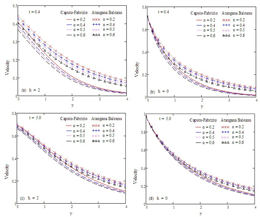
Figure 10. Velocity profiles with altered values of α and other parameters are ω = 0.2, G_r = 2, P_reff = 0.1, G_m = 0.75, k_p = 1.5, S_c = 0.5, and M = 0.9.

FIGURE 11

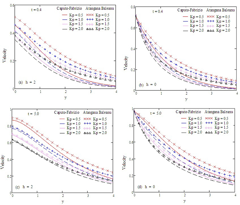
Figure 11. Velocity profiles with altered values of k_p and other parameters are ω = 0.2, G_r = 2, P_reff = 0.1, G_m = 0.75, α = 0.5, S_c = 0.5, and M = 0.9.

FIGURE 12

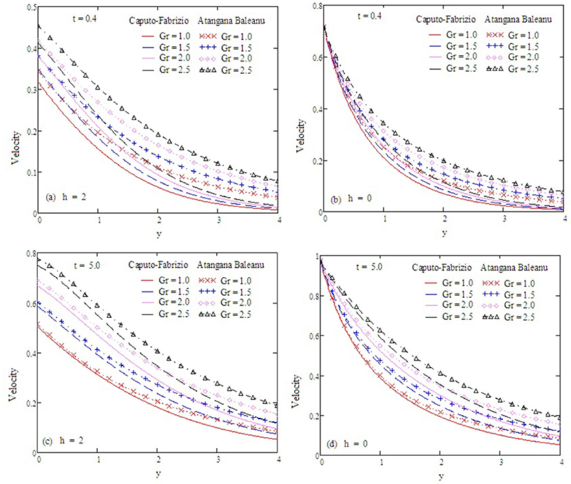
Figure 12. Velocity profiles with altered values of G_r and other parameters are ω = 0.2, α = 0.5, P_reff = 0.1, G_m = 0.75, k_p = 1.5, S_c = 0.5, and M = 0.9.

FIGURE 13

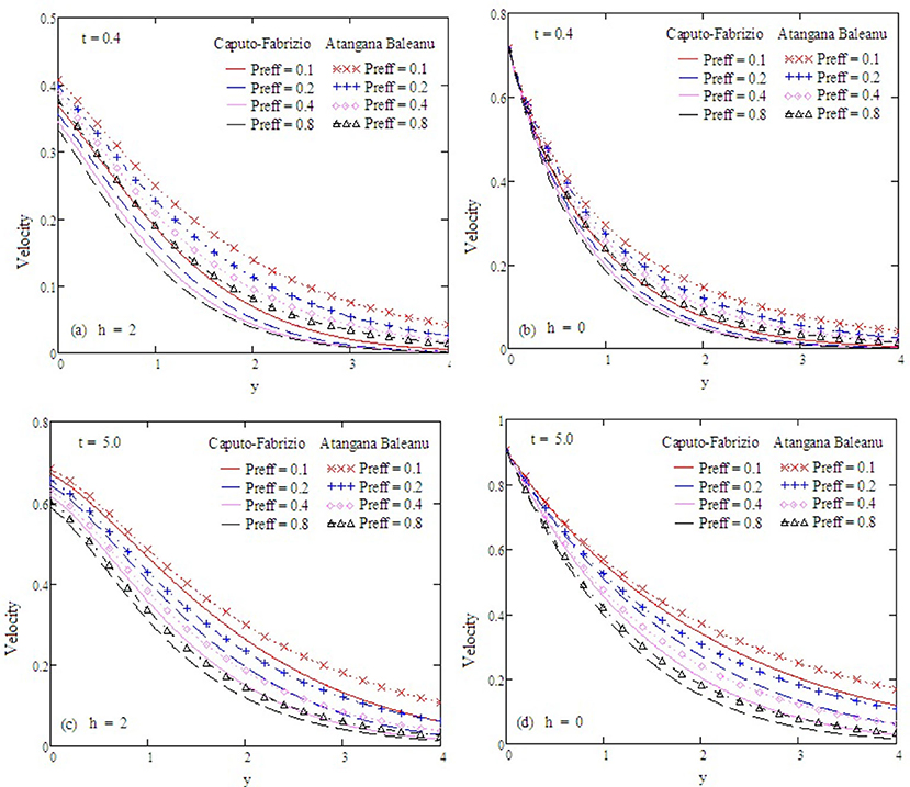
Figure 13. Velocity profiles with altered values of P_reff and other parameters are ω = 0.2, G_r = 2, M = 0.9, G_m = 0.75, α = 0.5, S_c = 0.5, and k_p = 1.5.

FIGURE 14

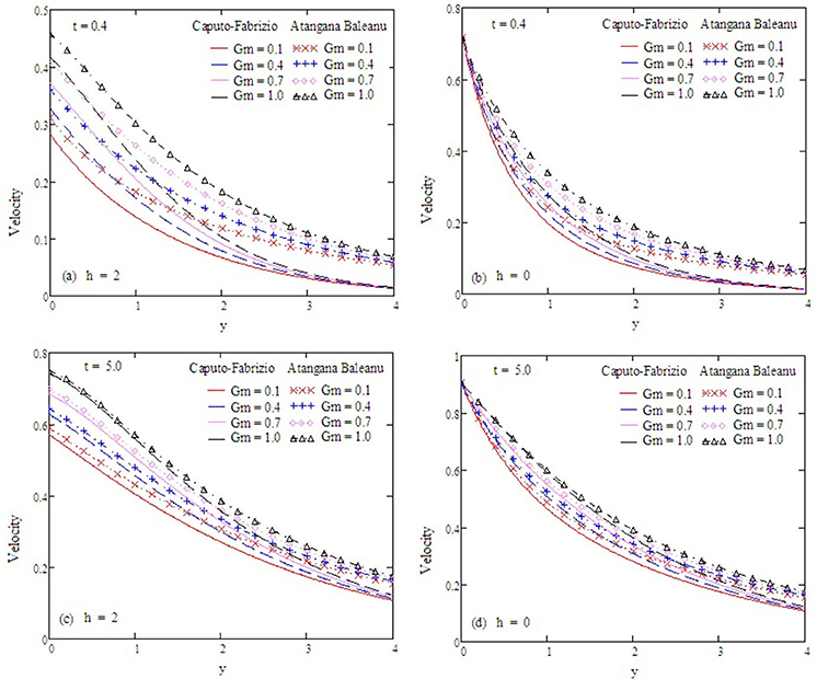
Figure 14. Velocity profiles with altered values of G_m and other parameters are ω = 0.2, G_r = 2, P_reff = 0.1, α = 0.5, k_p = 1.5, S_c = 0.5, and M = 0.9.

FIGURE 15

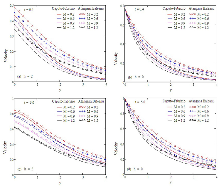
Figure 15. Velocity profiles with altered values of M and other parameters are ω = 0.2, G_r = 2, P_reff = 0.1, G_m = 0.75, α = 0.5, S_c = 0.5, and k_p = 1.5.

FIGURE 16

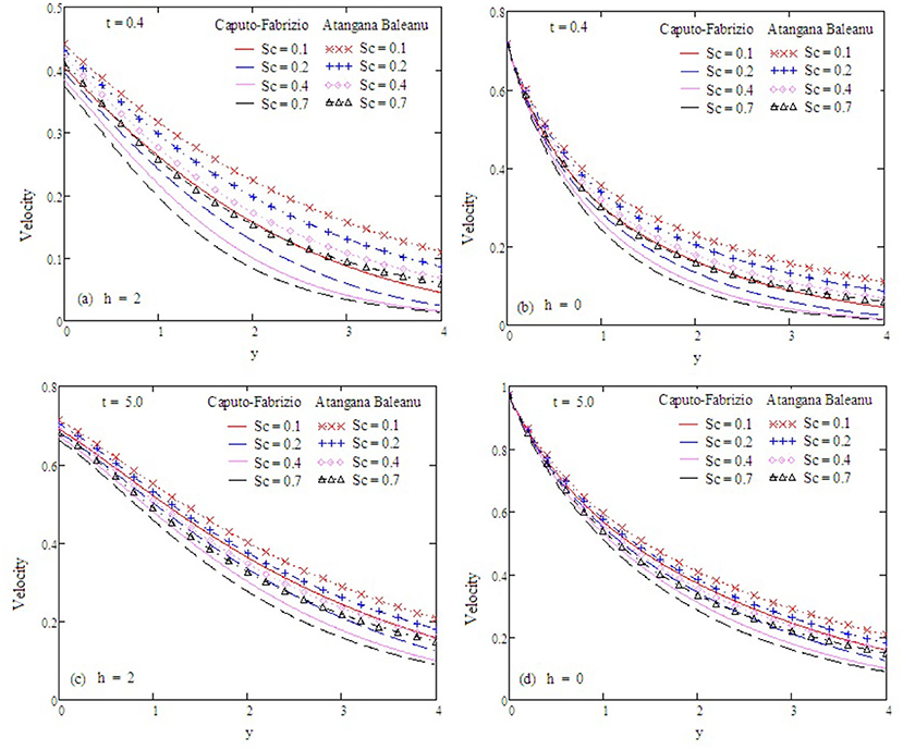
Figure 16. Velocity profiles with altered values of S_c and other parameters are ω = 0.2, G_r = 2, P_reff = 0.1, G_m = 0.75, α = 0.5, M = 0.9, and k_p = 1.5.

7. Conclusion

Ramped wall velocity and temperature conditions had a significant impact on MHD fractional Oldroyd-B fluid over a infinite vertical plate on a permeable surface. Fractional derivative operators are used to find the analytical solution using the Laplace transformation and inversion algorithm. Fluid velocity was analyzed through graphical results with the effect of different physical parameters. The main points of this problem are:

• The ABC fractional derivative is more significant compared to the classical model and other fractional models.

• The magnitude of the velocity increases with an increase in the fractional parameter α.

• The relationship between fractional parameters α and γ are reversed.

• Retardation time and relaxation time have a strong impact on the motion of fluid velocity.

• Velocity enhances with an increase in the value of λ_r.

• The relationship between λ and λ_r is the opposite to each other.

• The fluid velocity decreases with a large value of P_r.

• In the velocity field, the velocity reduces with the expansion of M.

Data Availability Statement

All datasets generated for this study are included in the article/supplementary material.

Author Contributions

MR and DB: conceptualization, investigation, and final review and editing. MR, DB, and SS: methodology. MG: software. SS: formal analysis. SS and MG: resources and original draft preparation. All authors contributed to the article and approved the submitted version.

Conflict of Interest

The authors declare that the research was conducted in the absence of any commercial or financial relationships that could be construed as a potential conflict of interest.

The handling editor declared a past co-authorship with the author DB.

References

1. Das K, Jana S. Heat and mass transfer effects on unsteady MHD free convection flow near moving vertical plate in porous medium. Bull Soc Math Banja Luka. (2010) 17:15–32.

Google Scholar

2. Hayat T, Khan I, Ellahi R, Fetecau C. Some MHD flows of a second grade fluid through the porous medium. J Por Media. (2008) 11:389–400. doi: 10.1615/JPorMedia.v11.i4.50

CrossRef Full Text | Google Scholar

3. Chandrakala P. Radiation effects on flow past an impulsively started vertical oscillating plate with uniform heat flux. Int J Dyn Fluids. (2011) 7:1–8.

Google Scholar

4. Narahari M, Nayan MY. Free convection flow past an impulsively started infinite vertical plate with Newtonian heating in the presence of thermal radiation and mass diffusion. Turk J Eng Environ Sci. (2011) 35:187–98.

Google Scholar

5. Chandran P, Sacheti NC, Singh AK. Natural convection near a vertical plate with ramped wall temperature. Heat Mass Trans. (2005) 41:459–64. doi: 10.1007/s00231-004-0568-7

CrossRef Full Text | Google Scholar

6. Narahari M, Beg OA, Ghosh SK. Mathematical modelling of mass transfer and free convection current effects on unsteady viscous flow with ramped wall temperature. World J Mech. (2011) 1:176–84. doi: 10.4236/wjm.2011.14023

CrossRef Full Text | Google Scholar

7. Toki CJ, Tokis JN. Exact solutions for the unsteady free convection flows on a porous plate with time-dependent heating. ZAMM Z Angew Math Mech. (2007) 87:4–13. doi: 10.1002/zamm.200510291

CrossRef Full Text | Google Scholar

8. Senapati N, Dhal RK, Das TK. Effects of chemical reaction on free convection MHD flow through porous medium bounded by vertical surface with slip flow region. Am J Comput Appl Math. (2012) 2:124–35. doi: 10.5923/j.ajcam.20120203.10

CrossRef Full Text | Google Scholar

9. Khan I, Fakhar K, Sharidan S. Magnetohydrodynamic free convection flow past an oscillating plate embedded in a porous medium. J Phys Soc Jpn. (2011) 80:1–10. doi: 10.1143/JPSJ.80.104401

CrossRef Full Text | Google Scholar

10. Das SS, Maity M, Das JK. Unsteady hydromagnetic convective flow past an infinite vertical porous flat plate in a porous medium. Int J Energy Environ. (2012) 3:109–18.

Google Scholar

11. Narahari M, Ishaq A. Radiation effects on free convection flow near a moving vertical plate with Newtonian heating. J Appl Sci. (2011) 11:1096–104. doi: 10.3923/jas.2011.1096.1104

CrossRef Full Text | Google Scholar

12. Kumar D, Singh J, Baleanu D. A fractional model of convective radial fins with temperature-dependent thermal conductivity. Rom Rep Phys. (2017) 69:103–5.

Google Scholar

13. Gupta S, Kumar D, Singh J. MHD mixed convective stagnation point flow and heat transfer of an incompressible nanofluid over an inclined stretching sheet with chemical reaction and radiation. Int J Heat Mass Trans. (2018) 118:378–87. doi: 10.1016/j.ijheatmasstransfer.2017.11.007

CrossRef Full Text | Google Scholar

14. Khan A, Karim F, Khan I, Ali F, Khan D. Irreversibility analysis in unsteady flow over a vertical plate with arbitrary wall shear stress and ramped wall temperature. Results Phys. (2018) 8:1283–90. doi: 10.1016/j.rinp.2017.12.032

CrossRef Full Text | Google Scholar

15. Imran MA, Riaz MB, Shah NA, Zafar AA. Boundary layer flow of MHD generalized Maxwell fluid over an exponentially accelerated infinite vertical surface with slip and Newtonian heating at the boundary. Results Phys. (2018) 8:1061–7. doi: 10.1016/j.rinp.2018.01.036

CrossRef Full Text | Google Scholar

16. Fetecau C, Vieru D, Fetecau C, Akhtar S. General solutions for magneto-hydrodynamic natural convection flow with radiative heat transfer and slip condition over a moving plat. Z Naturforsch. (2013) 68:659–67. doi: 10.5560/zna.2013-0041

CrossRef Full Text | Google Scholar

17. Jha BK, Apere CA. Combined effect of hall and ion-slip currents on unsteady MHD couette flows in a rotating system. J Phys Soc Jpn. (2010) 79:1–9. doi: 10.1143/JPSJ.79.104401

CrossRef Full Text | Google Scholar

18. Seth GS, Mahato GK, Sakar S. MHD natural convection flow with radiative heat transfer past an impulsively moving vertical plate with ramped temperature in the presence of hall current and thermal diffusion. Int J Appl Mech Eng. (2013) 18:1201–20. doi: 10.2478/ijame-2013-0073

CrossRef Full Text | Google Scholar

19. Yavuz M, Bonyah E. New approaches to the fractional dynamics of schistosomiasis disease model. Phys A. (2019) 525:373–93. doi: 10.1016/j.physa.2019.03.069

CrossRef Full Text | Google Scholar

20. Yavuz M. Characterizations of two different fractional operators without singular kernel. Math Mod Nat Phen. (2019) 14:302. doi: 10.1051/mmnp/2018070

CrossRef Full Text | Google Scholar

21. Atangana A, Baleanu D. New fractional derivatives with nonlocal and non-singular kernel: theory and application to heat transfer model. Therm Sci. (2016) 20:18. doi: 10.2298/TSCI160111018A

CrossRef Full Text | Google Scholar

22. Abdelijawad T. Different type kernel H-fractional differences and their fractional H-sums. Chaos Solit Fract. (2018) 116:146–56. doi: 10.1016/j.chaos.2018.09.022

CrossRef Full Text | Google Scholar

23. Siyal A, Abra KA, Solangi MA. Thermodynamics of magnetohydrodynamic Brinkman fluid in porous medium. J Therm Anal Calori. (2019) 136:2295–304. doi: 10.1007/s10973-018-7897-0

CrossRef Full Text | Google Scholar

24. Riaz MB, Atangana A, Saeed ST. MHD free convection flow over a vertical plate with ramped wall temperature and chemical reaction in view of non-singular kernel. In: Dutta H, Ocak A, Atangana A, editors. Fractional Order Analysis Theory, Methods and Application. Wiley-Blackwell (2020), 253–79.

Google Scholar

25. Riaz MB, Saeed ST. Comprehensive analysis of integer order, Caputo-fabrizio and Atangana-Baleanu fractional time derivative for MHD Oldroyd-B fluid with slip effect and time dependent boundary condition. Dis Con Dyn Sys. (2020).

Google Scholar

26. Saeed ST, Riaz MB, Baleanu D, Abro KA. A mathematical study of natural convection flow through a channel with non-singular kernels: an application to transport phenomena. Alex Engg J. (2020) 59:2269–81. doi: 10.1016/j.aej.2020.02.012

CrossRef Full Text | Google Scholar

27. Ghalib MM, Zafar AA, Riaz MB, Hammouch Z, Shabbir K. Analytical approach for the steady MHD conjugate viscous fluid flow in a porous medium with nonsingular fractional derivative. Phys A. (2020) 554:123941. doi: 10.1016/j.physa.2019.123941

CrossRef Full Text | Google Scholar

28. Asjad MI, Aleem M, Riaz MB, Ali R, Khan I. A comprehensive report on convective flow of fractional (ABC) and (CF) MHD viscous fluid subject to generalized boundary conditions. Chaos Solit Fract. (2019) 118:274–89. doi: 10.1016/j.chaos.2018.12.001

CrossRef Full Text | Google Scholar

29. Stehfest H, Goethe JW. Numerical inversion of Laplace transformation. Commun ACM. (1970) 13:47–9. doi: 10.1145/361953.361969

CrossRef Full Text | Google Scholar