 Ingo Tews
95% of researchers rate our articles as excellent or good
Learn more about the work of our research integrity team to safeguard the quality of each article we publish.
Find out more
REVIEW article
Front. Phys. , 14 May 2020
Sec. Nuclear Physics
Volume 8 - 2020 | https://doi.org/10.3389/fphy.2020.00153
This article is part of the Research Topic The Future of Nuclear Structure: Challenges and Opportunities in the Microscopic Description of Nuclei View all 11 articles
In recent years, new astrophysical observations have provided a wealth of exciting input for nuclear physics. For example, the observations of two-solar-mass neutron stars put strong constraints on possible phase transitions to exotic phases in strongly interacting matter at high densities. Furthermore, the recent observation of a neutron-star merger in both the electromagnetic spectrum and gravitational waves has provided compelling evidence that neutron-star mergers are an important site for the production of extremely neutron-rich nuclei within the r-process. In the coming years, an abundance of new observations is expected, which will continue to provide crucial constraints on the nuclear physics of these events. To reliably analyze such astrophysical observations and extract information on nuclear physics, it is very important that a consistent approach to nuclear systems is used. Such an approach consists of a precise and accurate method to solve the nuclear many-body problem in nuclei and nuclear matter, combined with modern nuclear Hamiltonians that allow to estimate the theoretical uncertainties. Quantum Monte Carlo methods are ideally suited for such an approach and have been successfully used to describe atomic nuclei and nuclear matter. In this contribution, I will present a detailed description of Quantum Monte Carlo methods focusing on the application of these methods to astrophysical problems. In particular, I will discuss how to use Quantum Monte Carlo methods to describe nuclear matter of relevance to the physics of neutron stars.
There are four fundamental forces in nature: gravity, the electromagnetic force, the weak nuclear force, and the strong nuclear force. While gravity describes the motion of the largest systems that we can observe, i.e., celestial bodies in the solar system and beyond, over very long distances, it is the weakest of the four fundamental forces. On the other end of the spectrum, the strong nuclear force is the strongest of the fundamental forces, but it acts only over very short distances and describes the interactions of some of the smallest building blocks of nature. In particular, it determines how neutrons and protons interact to form, e.g., atomic nuclei that make up all the matter that surrounds us everyday.
The strong interaction is described by its fundamental theory, Quantum Chromodynamics (QCD). QCD describes the strong interaction in terms of six quarks and eight gluons, which are elementary particles in the standard model. At low energies, these elementary particles can not be observed in isolation. Instead, they are confined to form so-called hadrons: mesons, e.g., the pion, or baryons, e.g., neutrons and protons. Furthermore, at these energies QCD is non-perturbative. Hence, it is computationally very demanding and costly to describe nuclear systems in terms of quarks and gluons by solving QCD explicitly. While Lattice QCD, which is a numerical approach to solve QCD on finite space-time lattices, attempts to achieve exactly that, such calculations are limited to systems with small nucleon numbers A < 5 and/or for large values of the quark masses, where simulations become cheaper. Instead, at low energies it is a very good approximation to describe nuclear systems, e.g., atomic nuclei, in terms of protons and neutrons which interact via some effective model of strong interactions, i.e., nuclear forces. One of the major goals of theoretical nuclear physics is to unravel the exact nature of nuclear forces and to understand how these forces lead to the properties of the nuclear systems that we can observe.
Nuclear systems that can be explored in terrestrial laboratories are atomic nuclei, and nuclear theory tries to explain their structure, i.e, energy levels, radii, separation energies, decays, etc. (see, e.g., Hagen et al. [1], Elhatisari et al. [2], Lynn et al. [3], Klos et al. [4], Calci et al. [5], Piarulli et al. [6], Lonardoni et al. [7], and Gysbers et al. [8]). Of particular interest are exotic nuclei far from stability, because they probe nuclear interactions at larger proton-to-neutron asymmetries [9–12]. The Coulomb interaction does not allow the ratio of protons to neutrons, the proton fraction, to become too large because in such cases the Coulomb repulsion among the protons would overcome the short-range nuclear attraction and make nuclei fall apart. On the other hand, neutron-rich nuclei, which explore smaller proton fractions, can be bound in nature, but the most exotic among them are extremely short-lived. The limits of existence of these nuclei are described by the neutron dripline, where one- and two-neutron separation energies become negative [13].
Neutron-rich nuclei are relevant for the so-called rapid neutron-capture process (r-process), a nucleosynthesis process that creates nearly half of all the elements heavier than iron in the universe. Hence, neutron-rich nuclei are extensively studied in nuclear-structure calculations and experiments. Our experimental knowledge will be significantly expanded in experiments at the upcoming Facility for Radioactive Ion Beams (FRIB) in the US and the Facility for Antiproton and Ion Research (FAIR) in Germany. But even with these advanced facilities, exotic nuclei with the most extreme neutron-to-proton ratios will not live long enough to be studied experimentally. Hence, the determination of their properties, which are very important as input in r-process studies, relies on theoretical models and astrophysical observations [14]. To improve theoretical models, the interactions in many-body systems with small proton fractions need to be understood better and tested against experimental data where available.
Luckily, atomic nuclei are not the only systems where one can test nuclear interactions at neutron-rich extremes. Neutron stars, which are one of the final stages of stellar evolution, are supported against gravitational collapse by strong interactions among its constituents, mainly neutrons with only around 5–10% of protons. In addition, with typical masses of 1.4 times the mass of our sun compressed into a star with a radius of 11–12 km, the densities in the core of neutron stars are extremely high. While atomic nuclei explore densities of the order of the nuclear saturation density, which corresponds to a mass density of 2.7 · 1014 g/cm3, neutron stars explore strong interactions at much larger densities of up to 10 times nsat. Hence, neutron-star observations allow us to test nuclear interactions at low proton fractions and high densities, which provides important complimentary information to experiments here on Earth. As a consequence, the study of these astrophysical systems is very fascinating and important, and allows to probe nuclear interactions under extreme conditions.
The crucial quantity relating both experiments and astrophysical observations is the equation of state (EOS), which provides a relation between the energy density, pressure, temperature, and the proton fraction of the matter in nuclear systems. For neutron stars, due to the very high densities in these systems, the Fermi energy of the nucleons is typically much larger than thermal energies. For example, while neutron stars typically have temperatures of the order of T = 108 K, the corresponding thermal energy of about 10 keV is much smaller than typical particle energies of the order of a few tens of MeV. Hence, one can neglect thermal effects, except in the most catastrophic astrophysical scenarios. Then, the EOS is simply relating the energy density ϵ and the pressure P, or alternatively the energy per particle E/A and the baryon density n, for a given proton fraction x.
Astrophysical observations of neutron stars allow us to constrain the EOS, and hence, the strong interactions that determine its properties. In recent years, exciting new astrophysical observations of neutron-star properties have provided a wealth of input for nuclear physics, and I will address these observations in section 2.2. Additional observations in the coming years, for example by the Neutron-Star Interior Composition Explorer (NICER) mission that recently reported its first measurement [15, 16], will add even more information. However, if we want to reliably analyze such astrophysical observations with the goal of constraining the nuclear EOS, we need to relate observations and nuclear interactions in a consistent and model-agnostic way, to avoid any model-related biases and to minimize systematic uncertainties.
In a microscopic approach, one would start from a Hamiltonian that describes the interactions among the relevant degrees of freedom of the system at hand, and solve the many-body Schrödinger equation for that system (e.g., nucleonic matter in neutron stars). Such an approach should consist of a precise and accurate method to solve the nuclear many-body problem in nuclei and nuclear matter, combined with modern nuclear Hamiltonians that allow to estimate the theoretical uncertainties of the nuclear interactions. Quantum Monte Carlo (QMC) methods [17] are ideally suited for such an approach and have been successfully used to describe atomic nuclei and nuclear matter. On the other hand, chiral effective field theory (EFT) [18–21] provides a systematic expansion of the nuclear forces, that allows to estimate theoretical uncertainties.
In this contribution, I will present a detailed description of Quantum Monte Carlo methods, focusing on the application of these methods to astrophysical problems. In particular, I will discuss how to use Quantum Monte Carlo methods to describe nuclear matter of relevance to the physics of neutron stars. I will also discuss how the combination of these methods with systematic interactions from chiral EFT allows us to extract information on the nuclear EOS in a reliable fashion. This contribution is organized as follows. In section 2, I will review neutron stars and the most important recent neutron-star observations. In section 3, I will address how to study the nuclear matter in neutron stars using Quantum Monte Carlo methods and modern nuclear interactions. In section 4, I will then show results and explain how to use these results to study neutron stars. Finally, I will summarize in section 5.
In this section, I will review neutron stars and their relevant equations, as well as the most important recent neutron-star observations.
Neutron stars are one of the final stages of stellar evolution. While low-mass stars like our sun end their life as white dwarfs, neutron stars are remnants of core-collapse supernova explosions of medium-mass stars in the range of 8–20 solar masses (heavier stars will collapse to black holes; see, e.g., Fryer [22]). Hence, neutron stars are the most compact stars in the Universe.
While stars in their burning stages are supported against gravitational collapse by the thermal energy released in nuclear fusion, these processes have stopped in white dwarfs and neutron stars. White dwarfs are the remaining cores of lighter stars that have shed their outer layers. They typically consist of Carbon and/or Oxygen, and have masses of the order of the mass of our sun compressed to the size of a typical planet, with radii of the order of several 1, 000 km. Due to the resulting densities and the fermionic nature of electrons, the electrons in white dwarfs form a degenerate gas. It costs energy to compress this electron gas, leading to a degeneracy pressure exerted outwards that balances the gravitational force that otherwise would collapse the star. Such a degenerate electron gas can typically support a white dwarf with a maximum mass of ~ 1.4M⊙, the so-called Chandrasekhar mass [23]. If a white dwarf accretes mass and surpasses this limit, the electron pressure does not suffice anymore to stabilize the star against gravitational collapse. This is what happens in core-collapse supernovae of heavier stars, where the white-dwarf-like core collapses due to continued accretion of fusion products. This collapse then triggers the supernova explosion of the star.
As a consequence of the core collapse, the densities of the electrons and nuclei increase dramatically, leading to an increasing Fermi energy for the electrons. At some point, it becomes energetically favorable for protons in the core to absorb electrons and form neutrons, lowering the proton fraction. As the collapse continues, at the largest densities in the core neutron-rich nuclei begin to dissolve into free nucleons, mostly neutrons. The collapse is halted when the core reaches radii of the order km. The abrupt stop of the contraction causes a so-called bounce that ultimately leads to a supernova explosion and ejects the remaining outer layers of the star, leaving a dense remnant. Due to their small proton fraction of the order of 5–10%, these young stars are called proto-neutron stars. They will cool over time and form cold neutron stars. Similar to white dwarfs, neutron stars are stabilized against gravitational collapse by the degeneracy pressure of their fermionic constituents, the neutrons. The discovery of the neutron by Chadwick [24] led to the postulation of neutron stars [25] long before their discovery in the 1960s [26, 27].
To investigate how the degeneracy pressure exerted by the neutron gas stabilizes neutron stars, one needs to start from the equations that describe the neutron-star structure. A less compact cold star (e.g., a white dwarf) would be described by the following structure equations:
where P is the pressure, G is the gravitational constant, m is the mass, ϵ is the energy density, and r is the radial coordinate. The first equation describes hydrostatic equilibrium and states that the pressure exerted outwards has to match the gravitational force acting inwards. The second equation is the conservation of mass. These equations are derived within Newtonian gravity, but since neutron stars are very compact, the structure equations need to be modified by general-relativistic extensions of Equation (1). These are the so-called Tolman-Oppenheimer-Volkoff (TOV) equations [31, 32]:
where c is the speed of light. In the following, we will write all equations in natural units and set c = 1. The energy density for non-relativistic nucleonic matter is given by
Here, n is the baryon number density and mN the nucleon mass. The first term of the energy density reflects the rest-mass density, while the second term is the specific internal energy.
To solve the TOV equations, the only required input is a relation between the pressure P and the energy density ϵ. This relation is the EOS, P = P(ϵ). With the EOS as input, the TOV equations can be solved by integrating from the stars center at r = 0 (where P = Pc and m = 0) to the stars edge at radius R (where P = 0 and m(R) = M). Hereby, the central pressure Pc is an input parameter, that determines the mass M and the radius R for the given EOS. Solving the TOV equations for many different values for Pc maps out the mass-radius (MR) relation, that describes the radius of a NS for a given mass, see Figure 1 for an example EOS. The EOS and the resulting MR relations are in a 1-to-1 correspondence: given an EOS, one can predict the structure properties of neutron stars, but neutron-star observations also allow to determine the EOS.
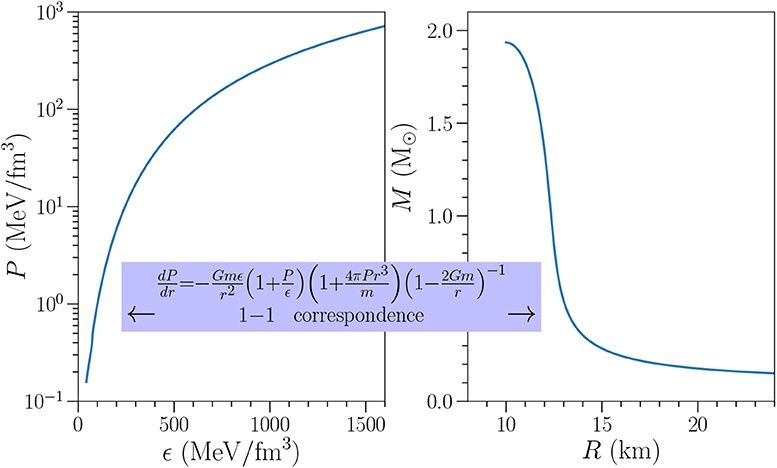
Figure 1. The equation of state (left) and the resulting mass-radius relation (right) upon solving the TOV equations for an example equation of state, i.e., the Skyrme model “NRAPR” constructed in Steiner et al. [28] which was fit to the APR equation of state of Akmal et al. [29]. Republished with permission of IOP Publishing, from Gandolfi et al. [30]; permission conveyed through Copyright Clearance Center, Inc.
Analogously to white dwarfs, Tolman and Oppenheimer inserted the EOS of a free and degenerate neutron gas to estimate the properties of neutron stars. They found a maximum mass of only 0.7M⊙ and, hence, concluded that neutron stars are not very important in nature. But, as we now know, the neutron-star EOS is much more complicated because strong interactions among neutrons, protons, and maybe other constituents at larger densities lead to many different effects. Including interaction effects can drastically increase the maximum mass of neutron stars to values as large as 3 − 4M⊙ [33], while observations have established the existence of neutron stars with masses as high as 2M⊙ (see next section). Hence, strong interactions are extremely important to stabilize neutron stars against gravitational collapse.
Generally, one can divide a neutron star into several layers. The neutron-star crust, the star's outer layer, can be separated into two regions. The outer crust consists of a lattice of neutron-rich nuclei of the iron region. With increasing density, these nuclei become more and more neutron-rich. At a density of approximately 4 · 1011 g/cm3, the inner crust begins. Here, the neutron chemical potential is so large that neutrons begin to drip out of the nuclei and form a neutron gas around the lattice of nuclei. With increasing density, the density of the neutron gas increases and the nuclei slowly dissolve. At the bottom of the inner crust, the lattice of nuclei can form exotic structures, called pasta phases, by merging into rods and slabs [34].
The crust connects to the neutron-star core at about half nuclear saturation density. Here, all nuclei have dissolved and the neutron star consists of a fluid of neutrons, protons, and electrons. At even larger densities, in the so-called inner core of neutron stars, exotic phases of matter might appear. The neutron-star might experience phase transitions to hyperonic matter [35], deconfined quark matter [36], or other exotic phases. However, there is no reliable experimental information on matter at such high densities and, hence, on the relevant degrees of freedom that are present in the neutron-star core. Therefore, theoretical models for the EOS have a large spread.
Due to the 1-to-1 correspondence between the EOS and the MR relation, neutron-star observations are an ideal way to constrain EOS models. While we can observe masses quite accurately, neutron-star radii are very uncertain, and typically range from 9−15 km for a typical 1.4M⊙ star [37]. This situation improves with new observations, e.g., from missions like NICER. For example, in the last years several observations have put tight constraints on the EOS and reduced the radius uncertainty quite dramatically. I will discuss these observations in the following, and show how they informed the EOS in section 4.
Neutron stars are typically observed as pulsars, i.e., rotating neutron stars that emit beams of electromagnetic signals (mostly radio signals) that can be detected on Earth. When these pulsars are in a binary with another star, it is possible to accurately measure the masses of the objects by making use of general-relativity effects, e.g., Shapiro delay [38]. As a consequence, neutron-star masses could historically be inferred quite precisely [37]. Neutron-star masses can provide strong EOS constraints because they require the EOS to be sufficiently stiff, i.e., the pressure inside the neutron star has to be sufficiently high to support a star of a certain mass against gravitational collapse. The heavier an observed neutron star is, the stiffer the EOS has to be. This can be used to rule out too soft EOS models, or EOS with very strong phase transitions that experience regions with a sudden and too strong softening.
Since the discovery of pulsars in the late 1960s, most neutron-star masses that were measured precisely are of the order of 1.4M⊙ [37]. This constraint is rather weak, and most EOS models can easily reproduce neutron stars of that mass. However, there have been a few exciting additional observations in the past decade. The first such observation was reported in 2008 [39, 40], when the mass of the binary pulsar J1903+0327 was determined to be of the order of 1.7M⊙. Only a few years later, in 2010, the first neutron star with a mass of the order of two solar masses was observed using Shapiro delay [41]: the pulsar PSR J1918-0642 with M = 1.97 ± 0.04M⊙. This value was later corrected to be M = 1.93 ± 0.02M⊙ [42]. In 2013, the existence of two-solar-mass neutron stars was firmly established with the observation of PSR J0348+0432 with a mass of M = 2.01 ± 0.04M⊙ [43]. Finally, only recently an even heavier neutron star was observed [44]: MSP J0740+6620 with a mass of M = 2.14 ± 0.10M⊙. These measurements put very strong constraints on the EOS of dense matter, and on possible phase transitions to exotic phases in strongly interacting matter at high densities.
In contrast to masses, it is quite difficult to infer neutron-star radii. X-ray observations, which are typically used to determine radii, have large uncertainties due to poorly understood systematics [45]. Recently, with the first observation of gravitational waves from a neutron-star merger and its electromagnetic counterpart [46, 47], a new possibility to constrain neutron-star radii was established.
As a consequence of general relativity, two neutron stars in a binary system emit gravitational waves. Hence, the system slowly looses energy and the distance of the two neutron stars slowly decreases. This leads to an even stronger emission of gravitational waves and so on. Finally, after a time scale of the order of gigayears, the two neutron stars will merge and form either a heavier neutron star or a black hole.
Neutron-star mergers are fascinating events because they simultaneously emit gravitational waves and electromagnetic signals in form of gamma-rays, X-rays, optical, infrared, to radio signals, and neutrinos. On August 17, 2017, the first such event was observed in gravitational waves and the electromagnetic spectrum [46–49]. The gravitational-wave signal was called GW170817 and I will focus on it in the following.
The crucial quantity that allows to extract radius information from neutron-star mergers is the tidal polarizability, Λ, which describes how a neutron star deforms under an external gravitational field, e.g., the field of the second neutron-star in a binary systems. The quadrupole deformation Qij of a star, given an external field Eij = −∂U(r)/∂xi∂xj with gravitational potential U(r), is given by Qij ~ ΛEij. The tidal polarizability depends on neutron-star properties as [52]
Here, k2 is the tidal Love number which is computed together with the Tolman-Oppenheimer-Volkoff equations; see, for example, Flanagan and Hinderer [52], Damour and Nagar [53], and Moustakidis et al.[54] for more details. For a neutron star of a given mass, one can immediately see that the tidal polarizability is strongly related to the radius of the neutron star. In particular, a larger neutron star will have a large tidal polarizability, while a small neutron star will have a small polarizability. In a neutron-star binary, one typically defines the binary tidal polarizability parameter as a mass-weighted average of the individual tidal polarizabilities,
where M1 and M2 are the individual masses of the two neutron stars, Λ1 and Λ2 are the two star's tidal polarizabilities, and Mtot is the total mass of the system. In the left panel of Figure 2, I show the correlation of the average radius of the two neutron stars in a binary with the binary tidal polarizability, in this case for a system like GW170817. However, such a relation exists for any neutron-star binary. By measuring from the gravitational-wave signal, one can constrain the radius.
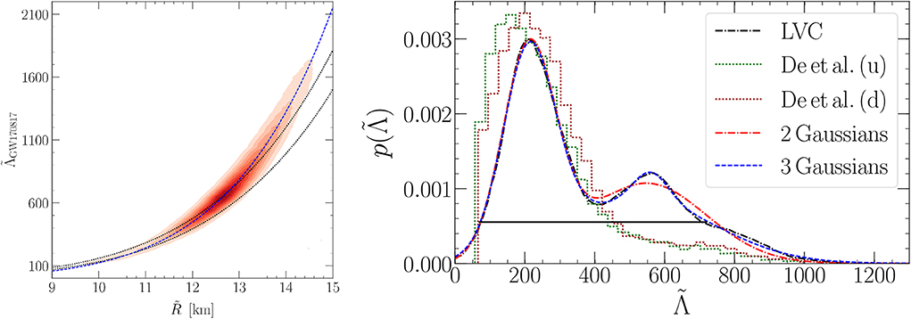
Figure 2. Left: Correlation between the average radius of the two neutron stars in GW170817 and the binary tidal polarizability . We show the distribution for the EOS models of Tews et al. [50] (red shaded area), a fit to this distribution (blue dashed line), as well as the result from Equation (5) of De et al. [51] with uncertainty (black dotted lines). Right: Marginalized and normalized posterior probability distribution for GW170817 from the LVC (black dashed-dotted line), from the analysis of De et al. [51] for the two extreme cases [uniform mass prior (u) and mass prior informed by double neutron stars (d)] (green and red dotted lines), and fits to the LVC distribution of Tews et al. [50] (red dashed-dotted and blue dashed lines). Reprinted by permission from Springer Nature, Tews et al. [50], copyright 2019.
The LIGO-Virgo collaboration (LVC) was able to observe the signal GW170817 for about 100s (several 1000 revolutions, starting from 25 Hz). A detailed analysis of the signal [49] allowed a precise determination of the chirp mass Mchirp, defined as
From the signal, the LVC could also extract the mass ratio q = M2/M1, where M1 is the mass of the heavier and M2 the mass of the lighter neutron star in the binary. Finally, several groups have analyzed the gravitational-wave data and provided posterior probability distributions for the binary tidal polarizability, . These probability distributions are normalized to 1 and are marginalized over the systems properties, like the EOS, the individual neutron-star masses and spins, etc. Hence, these distributions define the probability p that the two neutron stars in GW170817 had the binary tidal polarizability . I show the result from several extractions in the right panel of Figure 2.
In particular, I show the probability distributions extracted by the LVC [49] and from the analysis of De et al. [51] for the two extreme cases [uniform mass prior (u) and mass prior informed by double neutron stars (d)], as well as fits to the LVC distribution of Tews et al. [50]. In these analyses, parametric models for the EOS have been tested against the observed gravitational-wave data for varying system parameters using Bayesian statistical inference tools. The result of these analyses are multidimensional posterior functions for the tidal polarizability. Marginalizing over the various system parameters results in the function . For more details on the extractions I refer the reader to the corresponding references. Because the neutron-star deformation appreciably impacts the gravitational-wave signal only during the last few of several thousand observed orbits [52, 53], the uncertainty of the extracted tidal polarizability is rather large. In addition, there are ambiguities among several parameters, e.g., the neutron-star spins and the tidal polarizability, which additionally increase the uncertainties.
The results for were used by several groups to constrain the MR relation of neutron stars [55–59]. It was found that enforcing the constraint on rules out equations of state that are rather stiff and produce neutron stars with large radii. In particular, it was found that the radius of a 1.4M⊙ neutron star, R1.4, can be constrained to be R1.4 < 13.6 km. The observation of the first neutron-star merger, GW170817, was also very remarkable because the gravitational-wave signal was not the only observed signal. In addition, the electromagnetic counterpart, or kilonova, was observed in multiple wave lengths, and allows to impose additional constraints on the EOS. The kilonova seems to be inconsistent with a direct collapse of the merger remnant to a black hole and, hence, rules out very soft EOS that cannot support sufficiently large neutron-star masses [60]. The kilonova is also inconsistent with the formation of a long-lived neutron star [61] and, hence, rules out EOS with maximum masses larger than about 2.2–2.3 M⊙ [61, 62]. Hence, the kilonova observations seem to prefer a delayed collapse of the merger remnant to a black hole. I will discuss the impact of these observations later.
To constrain the neutron-star EOS from microscopic calculations, we need to understand the properties of the nuclear matter in the core of neutron stars. This system is described by a fluid of neutrons at nuclear densities with a small fraction of protons and electrons in β-equilibrium. Calculating the EOS of neutron-star matter is a challenging task because the interactions among nucleons are usually non-perturbative and have a complicated spin-isospin structure. Furthermore, given any nuclear interaction, an accurate and precise way of solving the many-body Schrödinger equation is needed to solve the many-body problem.
For strongly-interacting matter, there are several computational methods that have been used to solve the many-body problem. These methods include, for example, many-body perturbation theory (MBPT) [63–67], the coupled-cluster method [68], the self-consistent Green's function method [69, 70], or the Brueckner-Hartree-Fock approach [71]. Here, I illustrate how to calculate properties of the EOS of neutron stars using precise and accurate quantum Monte Carlo methods [17] combined with modern nuclear Hamiltonians that allow to estimate the theoretical uncertainties.
Quantum Monte Carlo methods are one among several many-body methods to solve the Schrödinger equation for strongly interacting nucleonic matter. In particular, QMC methods solve the nuclear many-problem non-perturbatively and with controlled approximations, which makes QMC methods quasi-exact. They have been very successfully used in studies of nuclear matter and light nuclei [17, 72]. Several implementations of QMC methods have been developed over the years, e.g., Green's function Monte Carlo (GFMC) [73] or auxiliary-field diffusion Monte Carlo (AFDMC) [74]. In this contribution, I will focus on the AFDMC method that has been used extensively to study nuclear matter for astrophysical applications [3, 33, 75–80].
The main idea of Quantum Monte Carlo methods is to stochastically solve the many-body Schrödinger equation to extract the ground state of a system, by evolving a given trial wave function of the many-body system, ΨV, in imaginary time τ = it,
Here, H is the Hamiltonian of the system, given by a collection of point-particles interacting via two-, three-, and other many-body forces (indicated by ellipses),
The first term is the nucleon kinetic energy with nucleon mass mN, vij is the nucleon-nucleon (NN) interaction, Vijk describes three-nucleon (3N) interactions, and so on. I will discuss the Hamiltonian in the next section.
When expanding the trial wave function ΨV in eigenfunctions of the Hamiltonian Φi, , one can rewrite Equation (7) as
where the index i = 0 describes the lowest-energy eigenstate in the trial wave function (typically the ground state of the system). As a consequence, when evolving ΨV in imaginary time as shown above, excited states (with Ei > E0) are exponentially suppressed and will be projected out from the trial wave function for evolutions to sufficiently large imaginary times. Only the Φ0 contribution will remain after this process. Hence, given a good trial wave function with overlap with the true ground state of the system, the imaginary-time evolution projects out this ground state and allows to access its properties.
Let us discuss this process in more detail. QMC methods formulate the many-body problem in coordinate space. Then, the many-body Schrödinger equation in imaginary time for N nucleons reads
where the vector R = {r1, …, rN, s1, …sN} contains the configurations of all N particles with respect to all degrees of freedom, i.e., their positions ri and their spin-isospin spinors si, that contain amplitudes for all possible spin-isospin states: |p ↑〉, |p ↓〉, |n ↑〉, and |n ↓〉. In bra and ket notation, n and p denote neutrons and protons, respectively, and the arrow-up and -down indicate spin-up and -down. One can rewrite the Schrödinger equation, and obtain the wave function at imaginary time τ, |Ψ(R, τ)〉, from the wave function at τ0 (which I set to τ0 = 0 in the following for simplicty) due to time evolution,
Projecting this equation into coordinate space and inserting a completeness relation, this leads to the general solution for the Schrödinger equation:
with the Green's function or propagator
Here, denotes the kinetic energy part of the Hamiltonian and the potential part. By solving this integral equation for large imaginary times, one projects out the ground state, as discussed before. The crucial ingredient to accomplish that task is to compute the Green's function.
The simplest case for the Green's function is given for the free system with vanishing interactions, V = 0. In this case, the propagator can be computed analytically:
Adding an interaction is non-trivial. Ideally, one would like to be able to compute the matrix elements for and separately, because the element for can be calculated analytically. However, and cannot simply be separated as they are both arguments of the exponential function. A solution is offered by the Trotter-Suzuki formula [81], which allows to simplify the propagator for a small timestep Δτ ≪ 1:
The smaller the imaginary time step, the smaller is the error of this approximation. This approximation is now used to calculate the propagator in Equation (13) for very large imaginary times τ, by splitting the total propagator into n small time steps, and using Equation (15) at each time step:
where the Ri describe paths in configuration space.
To add an interaction in Quantum Monte Carlo methods, it is important that the interactions are local, i.e., , and, thus, the potential is only a function of particle separations. In this case, the propagator for small time steps simplifies to
To write the propagator in this form, it is necessary to being able to separate all momentum dependencies as a quadratic term like above, which can generally be done only for local interactions. In this case, the interaction parts can be easily evaluated by exponentiating a small spin-isospin matrix. For non-local potentials, the evaluation of the propagator would involve the numerical calculation of derivatives, which is computationally too expensive.
Inserting this solution into Equation (12), one obtains
This equation is then solved consecutively for many small time steps until convergence is achieved. The remaining integrals are solved stochastically using Monte Carlo techniques, by averaging over a large number of configurations, or walkers, that are simultaneously evolved in imaginary time. Hence, this method is called Quantum Monte Carlo method. Each walker is propagated along a path sampled according to the Gaussian factor in the integral and observables are calculated once convergence is reached. During the evolution, additional techniques like importance sampling and branching are implemented to improve convergence and reduce the computational cost.
For fermionic systems of interest in nuclear physics, the wave function is antisymmetric and contains many changes in sign. Hence, the integrands in the previous QMC integrals are highly oscillatory and lead to very large statistical uncertainties, so that no information can be obtained from the calculation. This is known as the fermion sign problem. The QMC algorithms I discuss here need the trial wave function to have a definite sign to mediate the sign problem. In practice, the wave function space is split into regions of positive and negative wave functions, defining a nodal surface at which the wave function changes sign. Generally, walkers that cross the nodal surface are removed from the evolution. This approximation is called fixed-node approximation [82, 83]. A generalization of this approximation to complex wave functions is called constrained-path method [84–86], constraining the path of walkers to regions of space where the overlap of walker and the trial wave function has a positive real part. In the following, I will present results that were obtained using the constrained-path method.
To estimate the impact of this approximation, one can perform a so-called unconstrained evolution after the constrained-path evolution is completed. In this process, the approximation is abandoned and the walkers are allowed to cross the nodal surface. The simulation is performed until the sign problem creates noise that is too large. If a good trial wave function was chosen in the beginning of the QMC calculation, the change from the constrained to unconstrained result is very small, because the nodal surface of the trial wave function is sufficiently close to the nodal surface of the true ground state. In that case, the constrained-path approximation is good and leads to results close to the true answer.
In Figure 3, I show an example for the ground-state energy of 4He from Lynn et al. [89]. In the example, first a constrained-path evolution was performed using the GFMC method until an imaginary time of τ ≈ 0.5 MeV−1. It can be seen that the energy drops fast and levels off after sufficiently large imaginary times. At this point in the evolution, all excited state contributions have been projected out and differences to the true ground-state energy are due to the constrained-path approximation. Afterwards, an unconstrained evolution was performed, which is shown in more detail in the inset. The unconstrained evolution presents only a small correction to the constrained result, which highlights the quality of the trial wave function in this case. This does not need to be the case, as I show in the right panel of Figure 3, where the unconstrained evolution is presented for a calculation of 16O using AFDMC. In this case, the trial wave function leads to a constrained-path result far from the true ground state of the system (at τ = 0), and the unconstrained evolution is necessary to extract the final answer.
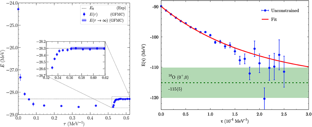
Figure 3. Left: The imaginary time evolution for the ground state energy of 4He in the GFMC method using the local chiral two- and three-nucleon interactions of Gezerlis et al. [87], Gezerlis et al. [88], and Lynn et al. [3] at cutoff R0 = 1.0 fm. The figure shows the constrained evolution, i.e., an evolution where the nodal surface is fixed, while the inset shows the unconstrained evolution. Reprinted figure with permission from Lynn et al. [89]. Copyright 2017 by the American Physical Society. Right: The unconstrained evolution for the ground-state energy of 16O in the AFDMC method (blue points) using the same local interactions. The red line represents an exponential fit to the data to extrapolate to the final result (green band). Reprinted figure with permission from Lonardoni et al. [90]. Copyright 2018 by the American Physical Society.
Typically, the unconstrained evolution is very important for nuclei and considered less important when calculating nuclear matter relevant for astrophysics. Hence, in the following I will only show results obtained using the constrained-path evolution. However, please see Piarulli et al. [79] for a recent analysis of the quality of the constrained-path approximation when calculating neutron matter with realistic Hamiltonians.
In the following, I will explain how a Quantum Monte Carlo calculation is done in practice. The first step of a QMC calculation of infinite matter is a Variational Monte Carlo (VMC) calculation. The VMC method is used to calculate the properties of the given many-body system starting from a trial wave function, ΨV, which is usually chosen of the form
where the factor FC accounts for all the central spin/isospin-independent correlations, and F2 and F3 are linear spin/isospin two- and three-body correlations; see Carlson et al. [17] for details. The part |Φ(R)〉 is usually given by a Slater determinant,
where the index α labels the single-particle states which depend on the studied system, and set the correct quantum numbers. For nuclear matter of interest here, |Φ〉 is built from a Slater determinant of plane-wave states with momenta ki. The ki are given by quantized momenta in a finite box with periodic boundary conditions, whose dimensions are determined by the chosen density and number of particles. The choice of periodic boundary conditions allows to study the infinite system [76]. The energy at the VMC level can be calculated as
and provides an upper bound to the true ground-state energy, E0 ≤ EV. Here, σ = {σ1…σN}, and τ = {τ1…τN} include all particles' spins σi, and isospins τi. The above equation can be written as
where P(R, σ, τ) is a probability distribution. Typically, one chooses, . The probability distribution P is then used to sample the configurations that are used to stochastically solve the multidimensional integral by employing Monte Carlo integration methods, e.g., the Metropolis algorithm.
It is obvious that the results of a VMC calculation depend strongly on the choice of the variational wave function, because no diffusion as described in the beginning of this section is performed. However, since the VMC method offers an upper bound to the true ground state of the system, it allows to improve the variational wave function for a given system, which feeds into all subsequent parts of the calculation. This is done by varying all the parameters that describe the trial wave function, e.g., the correlations in Equation (19), and minimizing the variational energy. For the optimal set of variational parameters, the optimized trial wave function serves as input for the next step of the calculation, where diffusion Monte Carlo methods are used to perform the imaginary time evolution.
The most accurate diffusion Monte Carlo technique is GFMC, where each walker contains not only the nucleon positions but also a complex amplitude for each possible spin-isospin configuration of the A nucleons including Z protons. In particular, in addition to the Monte Carlo integration over all spatial coordinates described above, summations in spin-isospin space are performed explicitly in GFMC. Because nuclear forces contain quadratic spin-isospin operators, components for all possible nucleon pairs have to be retained and accounted for explicitly. Hence, the scaling of the GFMC method with A is exponential, which makes it suitable to study light nuclei but unsuitable to study systems with large numbers of nucleons, like nucleonic matter. GFMC calculations are presently limited to 12 nucleons or 16 neutrons [91].
Instead, for nuclear matter discussed in this contribution, the AFDMC method [74] is more suitable. In AFDMC, all the summations in spin-isospin space are performed stochastically and quadratic spin-isospin dependences are linearized, which improves the scaling behavior but at the cost of less accuracy. This is made possible by using a Hubbard-Stratonovich transformation for an operator O,
As a consequence, dependences on spin-isospin operators can be changed from quadratic to linear, at the cost of additional integrations over the variables xi, called auxiliary fields. The Hubbard-Stratonovich transformation is exact when the integrals are exactly solved, but only statistically exact when Monte Carlo sampling is used like in the AFDMC method. As a consequence of applying the Hubbard-Stratonovich transformation, the wave function can be written as a product of single-particle spin-isospin states, which is a large simplification and improves the scaling behavior from exponential like in GFMC to linear or polynomial in the nucleon number A.
Following Schmidt and Fantoni [74] and considering only quadratic spin, isospin, and tensor operators, the potential can be written as
where the first term contains all spin-isospin-independent parts of the interaction, the second term absorbs the isospin-independent but spin-dependent parts, and so on. Here, Latin indices label nucleons and Greek indices label Cartesian components. For the m eigenvectors and eigenvalues of these matrices, one finds
For the matrices and the index m ranges from 1 to 3A, while there are A eigenvectors and eigenvalues for the matrix . Using this set of eigenvectors and the eigendecomposition of the A matrices, the potential can be rewritten as
where
The Hubbard-Stratonovich transformation is now applied to this interaction to linearize all spin-isospin dependences. Hence, wave functions only need to depend on single-particle spinors,
This allows to treat - nucleons in AFDMC.
When calculating nuclear matter, one typically simulates N particles in a cubic box with size L, where L is determined in such a way that the number density n in the box reflects a chosen value, L = (N/n)1/3. To avoid finite-size effects, the particle number N has to be chosen sufficiently large to probe the thermodynamic limit. As stated before, for nuclear matter the trial wave function is constructed from plane waves in a box with periodic boundary conditions (the implementation of twist-averaged boundary conditions [92] is currently explored). For periodic boundary conditions, the momenta are defined as . Here, the numbers nx, ny, and nz are integer numbers. In this case, the system acquires a shell structure, and the shell number is given by . Typically, since a homogenic and isotropic system is considered, calculations are only performed with closed shells. For I = 0 there is one combination of nx, ny, and nz, for I = 1 there are six combinations, etc. Then, shell closures are given for 1, 7, 19, 27, 33, etc. particles for a given spin-isospin configuration. In pure neutron matter, this leads to shell closures for N = 2, 14, 38, 54, 66, etc., as neutrons can be spin-up and spin-down. Due to growing computational costs associated with larger and larger particle numbers, for neutron matter one typically chooses N = 66 (33 spin up and 33 spin down neutrons). When comparing results for the free Fermi gas in a box as a function of particle number, it was found that N = 66 gives results close to the thermodynamic limit [75, 93].
In addition to the many-body method, it is necessary to specify a model for the nuclear interaction that defines the interaction terms in Equation (8). In the past, Quantum Monte Carlo methods have been used with phenomenological interactions of the Argonne type [94, 95] and 3N interactions of the Urbana [96] and Illinois [97] families with great success. However, the last years have seen the development of new local interactions within the framework of chiral effective field theory (EFT) [3, 87, 88, 98–100]. This enabled QMC calculations with a much greater number of nuclear interactions. While the interactions are not the focus of this review, in this section I briefly discuss local chiral interactions. For more details, I refer the reader to the more detailed reviews in Lynn et al. [72] and Piarulli et al. [101].
Chiral EFT [18–20] is a low-energy effective theory for QCD in terms of nucleon and pion degrees of freedom. It is naturally formulated in momentum space in terms of the momentum transfer q = p′ − p and the momentum transfer in the exchange channel, k = (p + p′)/2, where p and p′ are the average momenta of the incoming and outgoing particles. When performing a Fourier transformation to coordinate space, all q dependences transform to dependences on the relative distance of particles i and j, r = ri − rj and, hence, are local, while k dependences transform to gradients and, hence, non-localities. As a consequence, to implement a chiral interaction in QMC methods the interaction can only depend on q.
Chiral EFT is grounded in a separation of scales between the typical momentum scale of nucleons in nuclear systems Q, of the order of the pion mass, Q ~ mπ, and high-energy scales that denote the appearance of new degrees of freedom that are not explicitly accounted for in chiral EFT. The appearance of these high-energy degrees of freedom is marked by the so-called breakdown scale Λb, and beyond this scale, chiral EFT interactions can not be reliably employed in many-body calculations anymore. The nuclear interaction is then expanded in terms of according to a so-called power counting scheme. This scheme leads to a systematic expansion for nuclear interactions that makes chiral EFT very powerful. First, one can work up to a desired accuracy by going to higher and higher orders in the expansion. Second, one can estimate theoretical uncertainties based on the order-by-order contributions to a certain observable [102]. Another powerful advantage of chiral EFT interactions is that many-body forces naturally appear in the expansion and are intimately connected to the two-nucleon sector. This provides a systematic guiding principle to improve all individual parts of the nuclear Hamiltonian, in contrast to phenomenological interactions.
In chiral EFT, all the unresolved, short-range, high-energy physics beyond the breakdown scale is parameterized by a set of short-range contact operators among nucleons, which obey all the relevant symmetries [101]. For example, at leading order (LO), where ν = 0 and the interaction is momentum-independent, the contact part is given by
where the αi are low-energy couplings (LECs) that absorb the contributions of high-energy degrees of freedom. These LECs are typically fit once to experimental data, e.g., NN scattering phase shifts or cross sections. The resulting Hamiltonian can then be used to make predictions for all nuclear systems, e.g., the nuclear matter of interest to this contribution. At next-to-leading order (NLO), where ν = 2, the contact interactions are momentum-dependent:
where the γi are the LECs at NLO.
In addition to contact interactions, chiral EFT explicitly includes long-range pion exchange contributions. At LO for example, chiral interactions include the one-pion-exchange interaction (OPE), given in momentum space by
where gA is the axial-vector coupling constant of the nucleon, fπ is the pion decay constant, and mπ is the pion mass. Similarly to the short-range part, at higher orders more involved pion exchange contributions need to be accounted for.
These interactions are then Fourier transformed from momentum to coordinate space. To implement chiral interactions in QMC methods, local interactions need to be constructed. There are two sources of possible non-localities: (i) non-local operators that depend on k, see, e.g., Equation (34), or (ii) non-localities originating in the choice of so-called regulator functions, that are necessary in many-body calculations to cut off diverging momentum dependences.
The first source of non-localities can be avoided by choosing a local set of contact interactions. Let me explain the basic idea. Since chiral forces describe fermionic interactions that are typically used between antisymmetrized wave functions, it is intuitive to define the antisymmetrized interaction , with the antisymmetrizer
Constructing the antisymmetrized LO interaction, one obtains
Hence, one finds that if the LO chiral interactions are used between antisymmetrized wave functions, only two out of the four couplings are linearly independent. This is also intuitive, as the LO interactions describe the two possible S-wave scattering channels. As a consequence, it is sufficient to choose two out of the four operators and the common choice is
Similarly, at NLO, it is possible to choose only 7 out of the 14 operators given in Equation (34). To construct local interactions, one chooses the 6 local terms as well as the spin-orbit interaction ~ γ9 that can be treated within QMC methods. All the additional operator structures are then generated through antisymmetrization. Furthermore, pion-exchange interactions are local up to next-to-next-to-leading order (N2LO).
To avoid the non-localities due to the choice of regulator function, one typically defines these functions directly in coordinate space, e.g., by
where flong(r) is a long-range regulator and fshort(r) is a short-range regulator, and R0 is the cutoff scale. The long-range regulator function is applied to pion-exchange contributions, and cuts off short-range divergences ~ 1/r3n, while the short-range regulator smears out short-range delta-like contact interactions. When applying these regulator functions, regulator artifacts might appear that have to be carefully analyzed [103, 104].
It can be shown that it is possible to construct local chiral interactions up to N2LO [87, 88, 98, 100] using the ideas described above. These interactions can then be used in QMC methods. The N2LO interactions used in the following describe nucleon-nucleon phase shifts up to laboratory energies of 500 MeV within uncertainties, except the triplet D-wave phase shifts. To properly describe these phase shifts, it is necessary to construct interactions at next-to-next-to-next-to-leading order (N3LO), because only at that order D-wave contact interactions appear. At N3LO, however, only 8 out of 30 operators are local and, hence, there are too many non-local operators for this approach to work. Possible solutions are the definition of maximally local potentials [6], or the perturbative treatment of non-localities. The continued development of local chiral interactions is work in progress. However, I would like to stress that when describing neutron matter the triplet D waves vanish.
A detailed discussion of local interactions is not within the scope of this contribution and I refer the interested reader to Piarulli and Tews [101], where the derivation of local chiral interactions in both the delta-full and delta-less approaches (i.e, including explicitly delta-isobar degrees of freedom or not) is explained. In addition, Piarulli and Tews [101] explains the regularization scheme and appearing regulator artifacts in great detail. Local chiral interactions have been successfully used in calculations of nuclei [6, 7, 90] and I refer to Lynn et al. [72] for a review of recent results. In section 4, I will show how to use QMC calculations with chiral interactions to understand neutron stars.
Before discussing results, I would like to discuss strengths and weaknesses of the QMC approach with local chiral interactions compared to other many-body approaches mentioned before.
A major weakness of QMC methods is that they can only employ local interactions. This makes many contemporary nuclear Hamiltonians, especially many chiral Hamiltonians, not suitable at the moment. For example, as stated before, this currently limits the order of the chiral interactions employed in QMC methods to be below N3LO, while other many-body methods can typically employ interactions at higher orders. The need for local interactions presents a very strong limitation of QMC methods, and leads to additional problems, e.g., the appearance of regulator artifacts due to the violation of Fierz rearrangement freedom [104]. These regulator artifacts increase the uncertainties of the calculations [3].
However, even though QMC methods can only explore local interactions up to N2LO, they are capable of solving the many-body problem also for hard, high-cutoff interactions in an accurate and precise manner. While other many-body methods, can employ a wider range of interactions, they are typically limited to perturbative, low-cutoff interactions, for which these methods converge. Typically, bare chiral interactions have large Weinberg eigenvalues [105] and need to be softened to be implemented in most many-body methods. This is done by either employing low cutoffs of the order of 400 MeV from the start or by using softening transformations, e.g., the similarity RG (SRG). The ability to employ hard and/or bare interactions presents a major strength of QMC methods.
Work on constructing N3LO interactions for QMC methods is under way, see, e.g., Piarulli et al. [6]. Furthermore, work on high-cutoff local interactions is in progress, which will allow to explore cutoff regions where regulator choices become less important and where uncertainties from regulator artifacts are reduced [106].
To describe neutron stars, one needs access to the EOS, i.e., the relation of energy density and pressure; see section 2. In the following I will discuss how to extract this information from QMC simulations of nuclear matter.
Quantum Monte Carlo simulations are typically performed for A nucleons in a box with volume V = L3. The result of these simulations is the total energy per nucleon in the box, E/A, as a function of the number density n = A/V and the chosen proton fraction, x = np/(nn + np) = Z/A, where np is the proton density, nn is the neutron density, and Z is the number of protons in the box. The proton fraction determines the ratio of protons to neutrons, and is typically less than 10% in the core of neutron stars. Given the quantity E/A(n, x), it is easy to reconstruct the energy density and pressure:
The proton fraction is determined by the β-equilibrium between protons, neutrons, and electrons and results from the condition
where the μi are the chemical potentials of neutrons, protons, and electrons, respectively. The chemical potential can also be obtained from E/A(n, x). At a given density, Equation (42) determines the proton fraction x. Hence, if one calculates E/A(n, x), one can obtain p(n) and ϵ(n) in β-equilibrium, and from this the EOS.
Ideally, a calculation of E/A(n, x) at arbitrary proton fraction would be desirable to compute the EOS in β equilibrium. However, this is computationally expensive because several values of x would need to be computed for each density. Furthermore, with the addition of protons, interactions become more complicated to treat in QMC methods for nucleonic matter. For neutron stars, due to the small proton fraction, one generally starts from calculations of the pure neutron system with x = 0, called pure neutron matter (PNM), because the calculation is much easier as only certain parts of the interaction contribute. The AFDMC method is ideally suited to study pure neutron systems, and has been extensively used in the past for calculations of neutron drops and PNM [3, 33, 75, 76, 79, 99, 107, 108]. From PNM, one can typically extrapolate to small proton fractions by using empirical information from symmetric nuclear matter (SNM) with x = 1/2:
where S(n) = EPNM(n) − ESNM(n) is the symmetry energy and denotes the difference between SNM and PNM. The SNM EOS can be expanded around saturation density as
where E0 ≈ −16 MeV, n0 ≈ 0.16 fm−3, and K0 ≈ 230 MeV are empirical parameters that can be constrained experimentally. Using this information, the EOS of PNM can be easily extended to the small proton fractions of the order of 5% in β-equilibrium; see also Hebeler et al. [109]. I would like to note that, instead of using empirical values for the SNM parameters, it is also possible to calculate these parameters using QMC methods and local chiral interactions. This has very recently been achieved in Lonardoni et al. [80].
In Figure 4, I show AFDMC results for the energy per particle for 66 neutrons in a box as a function of density [3, 33]. The results have been obtained with local chiral interactions at N2LO with coordinate-space cutoff R0 = 1.0fm (red band), where the band denotes the theoretical uncertainty from the nuclear interactions as estimated from the order-by-order results [102]. In addition, the results are compared to results for astrophysical model EOS that are commonly used in astrophysical simulations: the Lattimer-Swesty EOS with incompressibility K = 220 [110], the TM1, SFHo, and SFHx EOSs (Hempel, private communication), the FSU and NL3 EOSs (Shen, private communication), and the DD2 EOS (Typel, private communication). It is obvious that the QMC calculations put strong constraints on the EOS of PNM, and disfavor several EOS, in particular EOS that lead to large pressures (large slopes of E/A with density). The L parameter, which is defined as the slope of the symmetry energy at saturation density and is connected to the pressure of PNM at saturation density, is found to lie in the range L = 24 − 68 MeV [80]. The calculation of PNM is now the starting point to construct the neutron-star EOS.
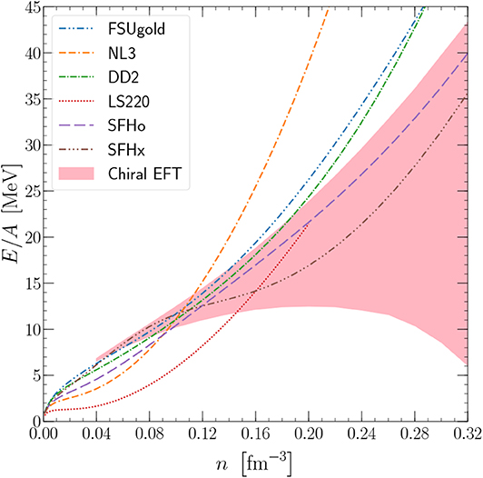
Figure 4. EOS of PNM obtained from QMC calculations with local chiral interactions at N2LO from Tews et al. [33]. The band indicates the theoretical uncertainty of the calculation, which mainly originates in the uncertainty of the nuclear interaction [3]. The chiral EFT band is compared with several model EOS for astrophysical calculations. Republished with permission of IOP Publishing, from Gandolfi et al. [30]; permission conveyed through Copyright Clearance Center, Inc.
To study neutron stars, we have to extend these calculations threefold. First, as discussed before, we have to extend the PNM EOS to finite proton fractions in β-equilibrium. Second, at low densities, neutron stars have a crust that consists of a lattice of nuclei and has to be taken into account. It is possible to replace the EOS at low densities, below ≈ 1/2nsat, with phenomenological crust EOS models. In Tews [111], I have shown how to use neutron-matter calculations and information on SNM to construct a crust EOS with theoretical uncertainties in the Wigner-Seitz approximation. In this approximation, the Wigner-Seitz cell is modeled as a nucleus with density nnuc and proton fraction xnuc surrounded by a pure neutron phase in equilibrium. The two phases can be modeled using the results of many-body calculations and I refer the reader to Tews [111] for more details. The results of this crust model are also in excellent agreement with phenomenological crust models. This crust EOS replaces the EOS at low densities. Third and final, as one can see in Figure 4, the uncertainty from calculations with chiral EFT interactions grows fast with density because momenta approach the breakdown scale. Beyond approximately 2nsat, calculations with local chiral interactions are not reliable anymore [33].
To reliably extract neutron-star properties, it is crucial to find a way of extending QMC calculations to higher density in a model-agnostic way, to avoid introducing any systematic uncertainties. In Tews et al. [33, 50, 59], we have developed an extension of QMC calculations to higher densities using the speed of sound cS; see also Greif et al. [112]. This extension uses the QMC calculations, extended to β-equilibrium and including a crust, up to a certain density ntr, which is varied between 1 − 2nsat. From these results, the speed of sound up to ntr is calculated. We do not know the speed of sound at higher densities, but we know that it has to be smaller then the speed of light, due to causality, and larger than 0, as the neutron star would otherwise be unstable: 0 ≤ cS ≤ c. Hence, by sampling many curves in the speed of sound plane, that are constrained up to ntr by QMC calculations and above by 0 ≤ cS ≤ c, we can gauge the uncertainty in the neutron-star EOS. In practice, we sample these curves as piecewise linear segments in the speed-of-sound plane. From the resulting curves for cS, we then can reconstruct the EOS and solve the TOV equations. The only observational requirement we enforce is that each EOS has to reproduce the heaviest observed neutron stars.
I show the resulting EOS envelopes in Figure 5 for ntr = nsat (left panel) and ntr = 2nsat (right panel). These envelopes include all EOS that are consistent with QMC calculations at low densities. The range where low-density constraints from QMC calculations are enforced can easily be identified from the plots. At larger densities, there is a great freedom for the EOS. However, even though uncertainties of the QMC calculations grow fast with density, the additional information from such calculations in the density range between 1 − 2nsat constrains the EOS significantly.
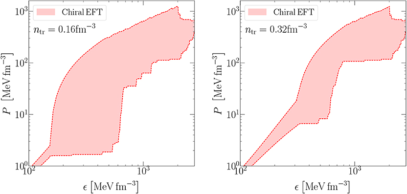
Figure 5. Equation-of-state envelopes for ntr = nsat (left) and ntr = 2nsat (right). Adapted by permission from Springer Nature, Tews et al. [50], copyright 2019.
Using these two sets of EOSs and solving the TOV equations (2), we can obtain the masses and radii of neutron stars as constrained by microscopic QMC calculations with uncertainty estimates from chiral EFT. We show the resulting MR envelopes in Figure 6 again for the cases ntr = nsat (left panel) and ntr = 2nsat (right panel). In the first case (left panel), the radius of a typical 1.4M⊙ neutron star is constrained to be between 8.4 − 15.2km. The maximum mass can reach values as high as 4 solar masses. It is interesting to note that the observation of heavy neutron stars directly impacts this uncertainty band, by ruling out too soft EOS. We indicate the excluded region by the gray-shaded area. The observation of heavier neutron stars, for example in Cromartie et al. [44], would allow to place even stronger constraints on soft EOS that produce low-radius neutron stars. Hence, neutron-star mass observations are a powerful tool to constrain the EOS of dense matter. However, even with such observations, the uncertainty remains quite large.
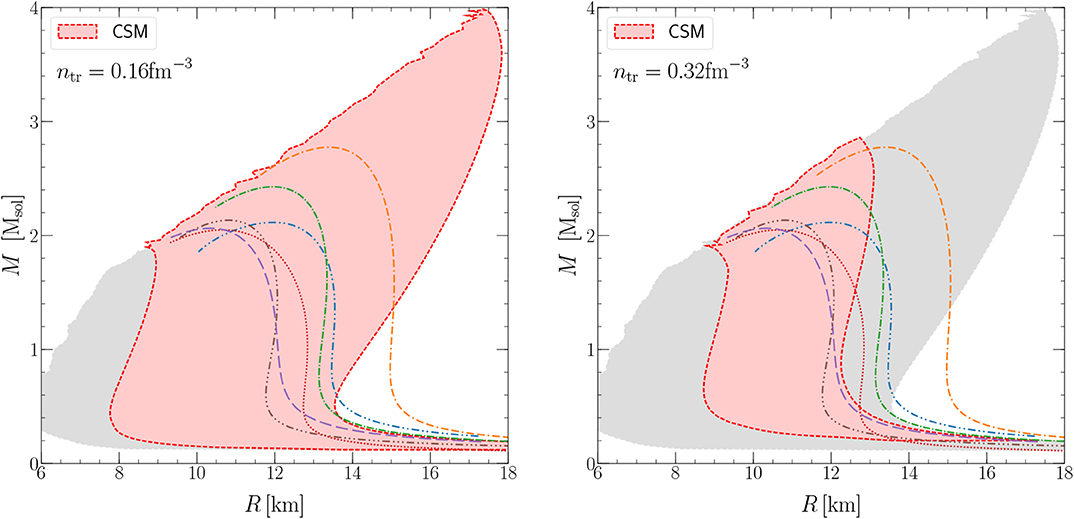
Figure 6. Mass-radius envelopes for ntr = nsat (left) and ntr = 2nsat (right). We show the EOS envelope given all constraints (red area), as well as the MR space that is ruled out by the two-solar mass constraint and/or when enforcing chiral EFT constraints up to larger densities (gray areas). The results are compared to the same EOSs shown in Figure 4. Adapted by permission from Springer Nature, Tews et al. [50], copyright 2019.
As in the EOS case, a possible improvement for the radius uncertainty is given by pushing the low-density constraints from QMC calculations to higher densities. We show the resulting MR envelope in the right panel of Figure 6 (for ntr = 2nsat), where the gray-shaded area is shown for comparison. It is found that the radius range for a typical neutron star reduces to 8.7 − 12.6km, much narrower than in the previous case. In this case, the upper limit on the maximum mass reduces to 2.9M⊙.
Finally, I address the recently observed neutron-star merger GW170817 [46–49] and its impact on inferring the MR relation. Using the information obtained from GW170817 and its electromagnetic counterpart, the EOS in our set can be analyzed according to their consistency with the gravitational-wave and EM signals. In particular, the EM signal constrains the EOS twofold: it disfavors a prompt collapse of the merger remnant to a black hole (which requires the maximum mass to be sufficiently large) [60, 61] and it disfavors a longer-lived neutron star as merger product (which requires the maximum mass to be sufficiently small) [61, 62]. This allows to constrain each EOS by computing its threshold mass for prompt collapse to a black hole [113, 114], Mthresh, comparing it with the total gravitational mass of GW170817, Mtot, and keeping only EOS where Mthresh > Mtot. Also, each EOS is required to have a maximum mass below 2.3M⊙ [61, 62]. Enforcing the gravitational-wave constraints as well as the constraints due to the energetics of the kilonova using a Bayesian analysis [115], this approach allows one to compute a posterior probability for each EOS in our EOS sets. I show the results in Figure 7.
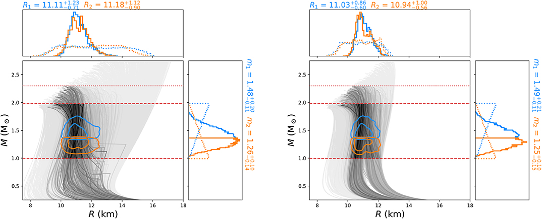
Figure 7. Mass-radius posteriors after constraints from the binary neutron-star merger GW170817 are enforced for the EOS set with ntr = nsat (left) and ntr = 2nsat (right). The shading of the individual MR curves corresponds to their posterior probability. The red-dashed lines indicate the mass range spanned by the prior, and the red-dotted line indicates the maximum neutron-star mass constraint as inferred from GW170817. The colored contours indicate the 50th and 90th percent credibility regions for the two neutron stars in GW170817, with the corresponding 1D marginalized posteriors plots on the sides. Figure taken from Capano et al. [115].
It is found that the gravitational-wave data from GW170817 constrains the maximum radius of neutron stars but is not informative for small radii [51, 116]. The observation of an electromagnetic counterpart for GW170817 and the deduction that there cannot have been a prompt collapse to a black hole, on the other hand, eliminates EOS that are too soft and produce a too small maximum mass, analogous to NS mass observations. This, in turn, places a lower limit on neutron-star radii. The upper limit on the maximum mass, however, does not significantly constrain the EOS posterior.
Assuming that local chiral EFT interactions remain valid up to nuclear saturation density, one finds that very stiff EOS can be ruled out by the tidal polarizability of GW170817. I show the results in the left panel of Figure 7. If, instead, local chiral EFT interactions remain valid up to twice nuclear saturation density, theoretical predictions for the EOS and gravitational-wave observations agree from the start, and enforcing gravitational-wave constraints does not impact the MR relation significantly (right panel of Figure 7). In both cases, the final results are consistent with each other and provide the most stringent constraints on the radius of a typical neutron star to date, .
In this review, I have discussed how to use QMC methods in combination with local interactions from chiral effective field theory up to N2LO to address the structure of neutron stars. I have shown how to obtain constraints on the EOS of dense matter, probed in the core of neutron stars, from microscopic calculations, and how these constraints impact the mass-radius relation. I have addressed the impact of the observation of heavy two-solar-mas neutron stars and the first observed binary neutron-star merger and its electromagnetic counterpart.
Quantum Monte Carlo methods have proven to be a reliable tool to investigate the EOS of neutron and neutron-star matter. Its recent combination with interactions from chiral effective field theory allows to build a systematic framework for the EOS with theoretical uncertainty estimates. However, current uncertainties are still sizable due to limitations in the employed interactions. Results for the mass-radius relation highlight that theoretical predictions need to be improved in the density range between 1 − 2nsat in order to provide accurate theoretical predictions of neutron-star structure observables. Work to improve the interactions is under way.
The author confirms being the sole contributor of this work and has approved it for publication.
This work was supported by the US Department of Energy, Office of Science, Office of Nuclear Physics, under Contract DE-AC52-06NA25396, the Los Alamos National Laboratory (LANL) LDRD program, and the NUCLEI SciDAC program. This research used resources provided by the Los Alamos National Laboratory Institutional Computing Program, which is supported by the U.S. Department of Energy National Nuclear Security Administration under Contract No. 89233218CNA000001, and the National Energy Research Scientific Computing Center (NERSC), a DOE Office of Science User Facility supported by the Office of Science of the U.S. Department of Energy under Contract No. DE-AC02-05CH11231.
The author declares that the research was conducted in the absence of any commercial or financial relationships that could be construed as a potential conflict of interest.
I thank my collaborators D. A. Brown, S. M. Brown, C. Capano, J. Carlson, S. De, E. Epelbaum, S. Gandolfi, A. Gezerlis, K. Hebeler, L. Huth, B. Krishnan, S. Kumar, J. Lippuner, D. Lonardoni, J. E. Lynn, B. Margalit, J. Margueron, A. Nogga, S. Reddy, K. E. Schmidt, A. Schwenk, and A. W. Steiner for their contributions to the studies presented in this work.
1. Hagen G, Ekström A, Forssén C, Jansen CR, Nazarewicz W, Papenbrock T, et al. Neutron and weak-charge distributions of the 48Ca nucleus. Nature Phys. (2015) 12:186–90. doi: 10.1038/nphys3529
2. Elhatisari S, Lee D, Rupak G, Epelbaum E, Krebs H, Lähde TA, et al. Ab initio alpha-alpha scattering. Nature. (2015) 528:111. doi: 10.1038/nature16067
3. Lynn JE, Tews I, Carlson J, Gandolfi S, Gezerlis A, Schmidt KE, et al. Chiral three-nucleon interactions in light nuclei, neutron-α scattering, and neutron matter. Phys Rev Lett. (2016) 116:062501. doi: 10.1103/PhysRevLett.116.062501
4. Klos P, Carbone A, Hebeler K, Menéndez J, Schwenk A. Uncertainties in constraining low-energy constants from3H β decay. Eur Phys J A. (2017) 53:168. doi: 10.1140/epja/i2017-12357-7
5. Calci A, Navrátil P, Roth R, Dohet-Eraly J, Quaglioni S, Hupin G. Can ab Initio Theory Explain the Phenomenon of Parity Inversion in 11Be? Phys Rev Lett. (2016) 117:242501. doi: 10.1103/PhysRevLett.117.242501
6. Piarulli M, Baroni A, Girlanda L, Kievsky A, Lovato A, Lusk E, et al. Light-nuclei spectra from chiral dynamics. Phys Rev Lett. (2018) 120:052503. doi: 10.1103/PhysRevLett.120.052503
7. Lonardoni D, Carlson J, Gandolfi S, Lynn JE, Schmidt KE, Schwenk A, et al. Properties of Nuclei up to A = 16 using Local Chiral Interactions. Phys Rev Lett. (2018) 120:122502. doi: 10.1103/PhysRevLett.120.122502
8. Gysbers P, Hagen G, Holt JD, Jansen JR, Morris TD, Navrátil P, et al. Discrepancy between experimental and theoretical β-decay rates resolved from first principles. Nat Phys. (2019) 15:428–31. doi: 10.1038/s41567-019-0450-7
9. Steppenbeck D, Takeuchi S, Aoi N, Doornenbal P, Matsushita M, Wang H, et al. Evidence for a new nuclear 'magic number' from the level structure of 54Ca. Nature. (2013) 502:207–10. doi: 10.1038/nature12522
10. Stroberg SR, Hergert H, Holt JD, Bogner SK, Schwenk A. Ground and excited states of doubly open-shell nuclei from ab initio valence-space Hamiltonians. Phys Rev C. (2016) 93:051301. doi: 10.1103/PhysRevC.93.051301
11. Liu HN, Obertelli A, Doornenbal P, Bertulani C, Hagen G, Holt JD, et al. How robust is the N = 34 subshell closure? First spectroscopy of 52Ar. Phys Rev Lett. (2019) 122:072502. doi: 10.1103/PhysRevLett.122.072502
12. Holt JD, Stroberg SR, Schwenk A, Simonis J. Ab initio limits of atomic nuclei. arXiv [Preprint] (2019). arXiv:1905.10475.
13. Erler J, Birge N, Kortelainen M, Nazarewicz W, Olsen E, Perhac AM, et al. The limits of the nuclear landscape. Nature. (2012) 486:509–12. doi: 10.1038/nature11188
14. Mumpower MR, Surman R, McLaughlin GC, Aprahamian A. The impact of individual nuclear properties on r-process nucleosynthesis. Prog Part Nucl Phys. (2016) 86:86–126. doi: 10.1016/j.ppnp.2015.09.001
15. Miller MC, Lamb FK, Dittmann AJ, Bogdanov S, Arzoumanian Z, Gendreau KC, et al. PSR J0030+0451 mass and radius from NICER data and implications for the properties of neutron star matter. Astrophys J Lett. (2019) 887:L24. doi: 10.3847/2041-8213/ab50c5
16. Riley TE, Watts AL, Bogdanov S, Ray PS, Ludlam RM, Guillot S, et al. A NICER view of PSR J0030+0451: millisecond pulsar parameter estimation. Astrophys J Lett. (2019) 887:L21. doi: 10.3847/2041-8213/ab481c
17. Carlson J, Gandolfi S, Pederiva F, Pieper SC, Schiavilla R, Schmidt KE, et al. Quantum Monte Carlo methods for nuclear physics. Rev Mod Phys. (2015) 87:1067–118. doi: 10.1103/RevModPhys.87.1067
18. Weinberg S. Nuclear forces from chiral Lagrangians. Phys Lett. (1990) B251:288–92. doi: 10.1016/0370-2693(90)90938-3
19. Weinberg S. Effective chiral Lagrangians for nucleon - pion interactions and nuclear forces. Nucl Phys. (1991) B363:3–18. doi: 10.1016/0550-3213(91)90231-L
20. Weinberg S. Three body interactions among nucleons and pions. Phys Lett. (1992) B295:114–21. doi: 10.1016/0370-2693(92)90099-P
21. Epelbaum E, Hammer HW, Meißner UG. Modern theory of nuclear forces. Rev Mod Phys. (2009) 81:1773–825. doi: 10.1103/RevModPhys.81.1773
22. Fryer CL. Mass limits for black hole formation. Astrophys J. (1999) 522:413. doi: 10.1086/307647
23. Chandrasekhar S. The maximum mass of ideal white dwarfs. Astrophys J. (1931) 74:81–2. doi: 10.1086/143324
25. Baade W, Zwicky F. Remarks on super-novae and cosmic rays. Phys Rev. (1934) 46:76–7. doi: 10.1103/PhysRev.46.76.2
26. Hewish A, Okoye SE. Evidence for an unusual source of high radio brightness temperature in the crab nebula. Nature. (1965) 207:59–60. doi: 10.1038/207059a0
27. Hewish A, Bell SJ, Pilkington JDH, Scott PF, Collins RA. Observation of a rapidly pulsating radio source. Nature. (1968) 217:709–13. doi: 10.1038/217709a0
28. Steiner AW, Prakash M, Lattimer JM, Ellis PJ. Isospin asymmetry in nuclei and neutron stars. Phys Rept. (2005) 411:325–75. doi: 10.1016/j.physrep.2005.02.004
29. Akmal A, Pandharipande VR, Ravenhall DG. The equation of state of nucleon matter and neutron star structure. Phys Rev C. (1998) 58:1804–28. doi: 10.1103/PhysRevC.58.1804
30. Gandolfi S, Lippuner J, Steiner AW, Tews I, Du X, Al-Mamun M. From the microscopic to the macroscopic world: from nucleons to neutron stars. J Phys. (2019) G46:103001. doi: 10.1088/1361-6471/ab29b3
31. Oppenheimer JR, Volkoff GM. On massive neutron cores. Phys Rev. (1939) 55:374–81. doi: 10.1103/PhysRev.55.374
32. Tolman RC. Static Solutions of Einstein's Field Equations for Spheres of Fluid. Phys Rev. (1939) 55:364–73. doi: 10.1103/PhysRev.55.364
33. Tews I, Carlson J, Gandolfi S, Reddy S. Constraining the speed of sound inside neutron stars with chiral effective field theory interactions and observations. Astrophys J. (2018) 860:149. doi: 10.3847/1538-4357/aac267
34. Ravenhall DG, Pethick CJ, Wilson JR. Structure of matter below nuclear saturation density. Phys Rev Lett. (1983) 50:2066–9. doi: 10.1103/PhysRevLett.50.2066
35. Lonardoni D, Lovato A, Gandolfi S, Pederiva F. Hyperon puzzle: hints from Quantum Monte Carlo calculations. Phys Rev Lett. (2015) 114:092301. doi: 10.1103/PhysRevLett.114.092301
36. Alford MG, Schmitt A, Rajagopal K, Schäfer T. Color superconductivity in dense quark matter. Rev Mod Phys. (2008) 80:1455–515. doi: 10.1103/RevModPhys.80.1455
37. Lattimer JM. The nuclear equation of state and neutron star masses. Ann Rev Nucl Part Sci. (2012) 62:485–515. doi: 10.1146/annurev-nucl-102711-095018
38. Shapiro II. Fourth Test of General Relativity. Phys Rev Lett. (1964) 13:789–91. doi: 10.1103/PhysRevLett.13.789
39. Champion DJ, Ransom SM, Lazarus P, Camilo F, Bassa C, Kaspi VM, et al. An eccentric binary millisecond pulsar in the galactic plane. Science. (2008) 320:1309–12. doi: 10.1126/science.1157580
40. Freire PCC, Bassa CG, Wex N, Stairs IH. On the nature and evolution of the unique binary pulsar J1903+0327. Mon Not R Astron Soc. (2011) 412:2763. doi: 10.1111/j.1365-2966.2010.18109.x
41. Demorest P, Pennucci T, Ransom S, Roberts M, Hessels J. Shapiro delay measurement of a two solar mass neutron star. Nature. (2010) 467:1081–3. doi: 10.1038/nature09466
42. Fonseca E, Pennucci TT, Ellis JA, Stairs IH, Nice DJ, Ransom SM, et al. The NANOGrav nine-year data set: mass and geometric measurements of binary millisecond pulsars. Astrophys J. (2016) 832:167. doi: 10.3847/0004-637X/832/2/167
43. Antoniadis J, Freire PCC, Wex N, Tauris TM, Lynch RS, van Kerkwijk MH, et al. A massive pulsar in a compact relativistic binary. Science. (2013) 340:6131. doi: 10.1126/science.1233232
44. Cromartie HT, Fonseca E, Ransom SM, Demorest PB, Arzoumanian Z, Blumer H, et al. Relativistic Shapiro delay measurements of an extremely massive millisecond pulsar. Nat Astron. (2019) 4:72–6. doi: 10.1038/s41550-019-0880-2
45. Ozel F, Freire P. Masses, Radii, and the Equation of State of Neutron Stars. Ann Rev Astron Astrophys. (2016) 54:401–40. doi: 10.1146/annurev-astro-081915-023322
46. Abbott BP, Abbott R, Abbott TD, Acernese F, Ackely K, Adams C, et al. GW170817: observation of gravitational waves from a binary neutron star inspiral. Phys Rev Lett. (2017) 119:161101. doi: 10.1103/PhysRevLett.119.161101
47. Abbott BP, Abbott R, Abbott TD, Acernese F, Ackley K, Adams C, et al. Multi-messenger observations of a binary neutron star merger. Astrophys J. (2017) 848:L12. doi: 10.3847/2041-8213/aa91c9
48. Abbott BP, Abbott R, Abbott TD, Acernese F, Ackley K, Adams C, et al. Gravitational waves and gamma-rays from a binary neutron star merger: GW170817 and GRB 170817A. Astrophys J. (2017) 848:L13. doi: 10.3847/2041-8213/aa920c
49. Abbott BP, Abbott R, Abbott TD, Acernese F, Ackley K, Adams C, et al. Properties of the binary neutron star merger GW170817. Phys Rev X. (2019) 9:011001. doi: 10.1103/PhysRevX.9.011001
50. Tews I, Margueron J, Reddy S. Confronting gravitational-wave observations with modern nuclear physics constraints. Eur Phys J. (2019) A55:97. doi: 10.1140/epja/i2019-12774-6
51. De S, Finstad D, Lattimer JM, Brown DA, Berger E, Biwer CM. Tidal deformabilities and radii of neutron stars from the observation of GW170817. Phys Rev Lett. (2018) 121:091102. doi: 10.1103/PhysRevLett.121.091102
52. Flanagan EE, Hinderer T. Constraining neutron star tidal Love numbers with gravitational wave detectors. Phys Rev. (2008) D77:021502. doi: 10.1103/PhysRevD.77.021502
53. Damour T, Nagar A. Relativistic tidal properties of neutron stars. Phys Rev. (2009) D80:084035. doi: 10.1103/PhysRevD.80.084035
54. Moustakidis CC, Gaitanos T, Margaritis C, Lalazissis GA. Bounds on the speed of sound in dense matter, and neutron star structure. Phys Rev. (2017) C95:045801. doi: 10.1103/PhysRevC.95.045801
55. Annala E, Gorda T, Kurkela A, Vuorinen A. Gravitational-wave constraints on the neutron-star-matter Equation of State. Phys Rev Lett. (2018) 120:172703. doi: 10.1103/PhysRevLett.120.172703
56. Fattoyev FJ, Piekarewicz J, Horowitz CJ. Neutron skins and neutron stars in the multimessenger era. Phys Rev Lett. (2018) 120:172702. doi: 10.1103/PhysRevLett.120.172702
57. Most ER, Weih LR, Rezzolla L, Schaffner-Bielich J. New constraints on radii and tidal deformabilities of neutron stars from GW170817. Phys Rev Lett. (2018) 120:261103. doi: 10.1103/PhysRevLett.120.261103
58. Lim Y, Holt JW. Neutron star tidal deformabilities constrained by nuclear theory and experiment. Phys Rev Lett. (2018) 121:062701. doi: 10.1103/PhysRevLett.121.062701
59. Tews I, Margueron J, Reddy S. Critical examination of constraints on the equation of state of dense matter obtained from GW170817. Phys Rev C. (2018) 98:045804. doi: 10.1103/PhysRevC.98.045804
60. Bauswein A, Just O, Janka HT, Stergioulas N. Neutron-star radius constraints from GW170817 and future detections. Astrophys J. (2017) 850:L34. doi: 10.3847/2041-8213/aa9994
61. Margalit B, Metzger BD. Constraining the maximum mass of neutron stars from multi-messenger observations of GW170817. Astrophys J Lett. (2017) 850:L19. doi: 10.3847/2041-8213/aa991c
62. Shibata M, Zhou E, Kiuchi K, Fujibayashi S. Constraint on the maximum mass of neutron stars using GW170817 event. Phys Rev D. (2019) 100:023015. doi: 10.1103/PhysRevD.100.023015
63. Hebeler K, Lattimer JM, Pethick CJ, Schwenk A. Constraints on neutron star radii based on chiral effective field theory interactions. Phys Rev Lett. (2010) 105:161102. doi: 10.1103/PhysRevLett.105.161102
64. Coraggio L, Holt JW, Itaco N, Machleidt R, Marcucci LE, Sammarruca F. Nuclear-matter equation of state with consistent two- and three-body perturbative chiral interactions. Phys Rev C. (2014) 89:044321. doi: 10.1103/PhysRevC.89.044321
65. Wellenhofer C, Holt JW, Kaiser N, Weise W. Nuclear thermodynamics from chiral low-momentum interactions. Phys Rev C. (2014) 89:064009. doi: 10.1103/PhysRevC.89.064009
66. Holt JW, Kaiser N. Equation of state of nuclear and neutron matter at third-order in perturbation theory from chiral effective field theory. Phys Rev. (2017) C95:034326. doi: 10.1103/PhysRevC.95.034326
67. Drischler C, Hebeler K, Schwenk A. Chiral interactions up to next-to-next-to-next-to-leading order and nuclear saturation. Phys Rev Lett. (2019) 122:042501. doi: 10.1103/PhysRevLett.122.042501
68. Hagen G, Papenbrock T, Ekström A, Wendt KA, Baardsen G, Gandolfi S, et al. Coupled-cluster calculations of nucleonic matter. Phys Rev C. (2014) 89:014319. doi: 10.1103/PhysRevC.89.014319
69. Carbone A, Rios A, Polls A. Symmetric nuclear matter with chiral three-nucleon forces in the self-consistent Green's functions approach. Phys Rev C. (2013) 88:044302. doi: 10.1103/PhysRevC.88.044302
70. Carbone A, Cipollone A, Barbieri C, Rios A, Polls A. Self-consistent Green's functions formalism with three-body interactions. Phys Rev C. (2013) 88:054326. doi: 10.1103/PhysRevC.88.054326
71. Isaule F, Arellano HF, Rios A. Di-neutrons in neutron matter within a Brueckner-Hartree-Fock approach. Phys Rev C. (2016) 94:034004. doi: 10.1103/PhysRevC.94.034004
72. Lynn JE, Tews I, Gandolfi S, Lovato A. Quantum Monte Carlo methods in nuclear physics: recent advances. Ann Rev Nucl Part Sci. (2019) 69:279–305. doi: 10.1146/annurev-nucl-101918-023600
73. Carlson J. Greens function Monte Carlo study of light nuclei. Phys Rev C. (1987) 36:2026–33. doi: 10.1103/PhysRevC.36.2026
74. Schmidt KE, Fantoni S. A quantum Monte Carlo method for nucleon systems. Phys Lett B. (1999) 446:99–103. doi: 10.1016/S0370-2693(98)01522-6
75. Gandolfi S, Illarionov AY, Schmidt KE, Pederiva F, Fantoni S. Quantum Monte Carlo calculation of the equation of state of neutron matter. Phys Rev C. (2009) 79:054005. doi: 10.1103/PhysRevC.79.054005
76. Gandolfi S, Gezerlis A, Carlson J. Neutron matter from low to high density. Ann Rev Nucl Part Sci. (2015) 65:303–28. doi: 10.1146/annurev-nucl-102014-021957
77. Buraczynski M, Gezerlis A. Ab initio and phenomenological studies of the static response of neutron matter. Phys Rev C. (2017) 95:044309. doi: 10.1103/PhysRevC.95.044309
78. Riz L, Pederiva F, Gandolfi S. Spin response and neutrino mean free path in neutron matter. J Phys G. (2020) 47:045106. doi: 10.1088/1361-6471/ab6520
79. Piarulli M, Bombaci I, Logoteta D, Lovato A, Wiringa RB. Benchmark calculations of pure neutron matter with realistic nucleon-nucleon interactions. Phys Rev C. (2020) 101:045801. doi: 10.1103/PhysRevC.101.045801
80. Lonardoni D, Tews I, Gandolfi S, Carlson J. Nuclear and neutron-star matter from local chiral interactions. arXiv [Preprint] (2019). arXiv:1912.09411.
81. Suzuki M. On the convergence of exponential operators- the Zassenhaus formula, BCH formula and systematic approximants. Comm Math Phys. (1977) 57:193–200. doi: 10.1007/BF01614161
83. Schmidt KE, Kalos MH. Applications of the Monte Carlo method in statistical physics. In: Binder K, editor. Topics in Current Physics, Vol. 36. New York, NY; Berlin; Heidelberg: Springer-Verlag (1984). p. 125–43. doi: 10.1007/978-3-642-96788-7
84. Zhang S, Carlson J, Gubernatis JE. Constrained path Quantum Monte Carlo method for fermion ground states. Phys Rev Lett. (1995) 74:3652–5. doi: 10.1103/PhysRevLett.74.3652
85. Zhang S, Carlson J, Gubernatis JE. Constrained path Monte Carlo method for fermion ground states. Phys Rev B. (1997) 55:7464–77. doi: 10.1103/PhysRevB.55.7464
86. Zhang S, Krakauer H. Quantum Monte Carlo method using phase-free random walks with slater determinants. Phys Rev Lett. (2003) 90:136401. doi: 10.1103/PhysRevLett.90.136401
87. Gezerlis A, Tews I, Epelbaum E, Gandolfi S, Hebeler K, Nogga A, et al. Quantum Monte Carlo calculations with chiral effective field theory interactions. Phys Rev Lett. (2013) 111:032501. doi: 10.1103/PhysRevLett.111.032501
88. Gezerlis A, Tews I, Epelbaum E, Freunek M, Gandolfi S, Hebeler K, et al. Local chiral effective field theory interactions and quantum Monte Carlo applications. Phys Rev C. (2014) 90:054323. doi: 10.1103/PhysRevC.90.054323
89. Lynn JE, Tews I, Carlson J, Gandolfi S, Gezerlis A, Schmidt KE, et al. Quantum Monte Carlo calculations of light nuclei with local chiral two- and three-nucleon interactions. Phys Rev C. (2017) 96:054007. doi: 10.1103/PhysRevC.96.054007
90. Lonardoni D, Gandolfi S, Lynn JE, Petrie C, Carlson J, Schmidt KE, et al. Auxiliary field diffusion Monte Carlo calculations of light and medium-mass nuclei with local chiral interactions. Phys Rev C. (2018) 97:044318. doi: 10.1103/PhysRevC.97.044318
92. Lin C, Zong FH, Ceperley DM. Twist-averaged boundary conditions in continuum quantum Monte Carlo. Phys Rev E. (2001) 64:016702. doi: 10.1103/PhysRevE.64.016702
93. Sarsa A, Fantoni S, Schmidt KE, Pederiva F. Neutron matter at zero temperature with auxiliary field diffusion Monte Carlo. Phys Rev. (2003) C68:024308. doi: 10.1103/PhysRevC.68.024308
94. Wiringa RB, Stoks VGJ, Schiavilla R. Accurate nucleon-nucleon potential with charge-independence breaking. Phys Rev C. (1995) 51:38–51. doi: 10.1103/PhysRevC.51.38
95. Wiringa RB, Pieper SC. Evolution of nuclear spectra with nuclear forces. Phys Rev Lett. (2002) 89:182501. doi: 10.1103/PhysRevLett.89.182501
96. Pudliner BS, Pandharipande VR, Carlson J, Wiringa RB. Quantum Monte Carlo Calculations of A ≤ 6 Nuclei. Phys Rev Lett. (1995) 74:4396. doi: 10.1103/PhysRevLett.74.4396
97. Pieper SC, Pandharipande VR, Wiringa RB, Carlson J. Realistic models of pion exchange three nucleon interactions. Phys Rev C. (2001) 64:014001. doi: 10.1103/PhysRevC.64.014001
98. Piarulli M, Girlanda L, Schiavilla R, Navarro Prez R, Amaro JE, Ruiz Arriola E. Minimally nonlocal nucleon-nucleon potentials with chiral two-pion exchange including Δ resonances. Phys Rev C. (2015) 91:024003. doi: 10.1103/PhysRevC.91.024003
99. Tews I, Gandolfi S, Gezerlis A, Schwenk A. Quantum Monte Carlo calculations of neutron matter with chiral three-body forces. Phys Rev C. (2016) 93:024305. doi: 10.1103/PhysRevC.93.024305
100. Piarulli M, Girlanda L, Schiavilla R, Kievsky A, Lovato A, Marcucci LE, et al. Local chiral potentials with Δ-intermediate states and the structure of light nuclei. Phys Rev C. (2016) 94:054007. doi: 10.1103/PhysRevC.94.054007
101. Piarulli M, Tews I. Local nucleon-nucleon and three-nucleon interactions within chiral effective field theory. Front Phys. (2020) 7:245. doi: 10.3389/fphy.2019.00245
102. Epelbaum E, Krebs H, Meißner UG. Improved chiral nucleon-nucleon potential up to next-to-next-to-next-to-leading order. Eur Phys J A. (2015) 51:53. doi: 10.1140/epja/i2015-15053-8
103. Dyhdalo A, Furnstahl RJ, Hebeler K, Tews I. Regulator artifacts in uniform matter for chiral interactions. Phys Rev C. (2016) 94:034001. doi: 10.1103/PhysRevC.94.034001
104. Huth L, Tews I, Lynn JE, Schwenk A. Analyzing the Fierz rearrangement freedom for local chiral two-nucleon potentials. Phys Rev C. (2017) 96:054003. doi: 10.1103/PhysRevC.96.054003
105. Hoppe J, Drischler C, Furnstahl RJ, Hebeler K, Schwenk A. Weinberg eigenvalues for chiral nucleon-nucleon interactions. Phys Rev C. (2017) 96:054002. doi: 10.1103/PhysRevC.96.054002
106. Tews I, Huth L, Schwenk A. Large-cutoff behavior of local chiral effective field theory interactions. Phys Rev C. (2018) 98:024001. doi: 10.1103/PhysRevC.98.024001
107. Gandolfi S, Carlson J, Pieper SC. Cold neutrons trapped in external fields. Phys Rev Lett. (2011) 106:012501. doi: 10.1103/PhysRevLett.106.012501
108. Maris P, Vary JP, Gandolfi S, Carlson J, Pieper SC. Properties of trapped neutrons interacting with realistic nuclear Hamiltonians. Phys Rev C. (2013) 87:054318. doi: 10.1103/PhysRevC.87.054318
109. Hebeler K, Lattimer JM, Pethick CJ, Schwenk A. Equation of state and neutron star properties constrained by nuclear physics and observation. Astrophys J. (2013) 773:11. doi: 10.1088/0004-637X/773/1/11
110. Lattimer JM, Swesty FD. A Generalized equation of state for hot, dense matter. Nucl Phys A. (1991) 535:331–76. doi: 10.1016/0375-9474(91)90452-C
111. Tews I. Spectrum of shear modes in the neutron-star crust: Estimating the nuclear-physics uncertainties. Phys Rev C. (2017) 95:015803. doi: 10.1103/PhysRevC.95.015803
112. Greif SK, Raaijmakers G, Hebeler K, Schwenk A, Watts AL. Equation of state sensitivities when inferring neutron star and dense matter properties. Mon Not Roy Astron Soc. (2019) 485:5363–76. doi: 10.1093/mnras/stz654
113. Bauswein A, Baumgarte TW, Janka HT. Prompt merger collapse and the maximum mass of neutron stars. Phys Rev Lett. (2013) 111:131101. doi: 10.1103/PhysRevLett.111.131101
114. Koppel S, Bovard L, Rezzolla L. A general-relativistic determination of the threshold mass to prompt collapse in binary neutron star mergers. Astrophys J. (2019) 872:L16. doi: 10.3847/2041-8213/ab0210
115. Capano CD, Tews I, Brown SM, Margalit B, De S, Kumar S, et al. Stringent constraints on neutron-star radii from multimessenger observations and nuclear theory. Nat. Astron. (2019) 8. doi: 10.1038/s41550-020-1014-6
Keywords: neutron stars, dense-matter equation of state, nuclear interactions, chiral effective field theory, ab-initio calculations, Quantum Monte Carlo methods
Citation: Tews I (2020) Quantum Monte Carlo Methods for Astrophysical Applications. Front. Phys. 8:153. doi: 10.3389/fphy.2020.00153
Received: 06 January 2020; Accepted: 15 April 2020;
Published: 14 May 2020.
Edited by:
Luigi Coraggio, National Institute of Nuclear Physics of Naples, ItalyReviewed by:
Francesca Sammarruca, University of Idaho, United StatesCopyright © 2020 Tews. This is an open-access article distributed under the terms of the Creative Commons Attribution License (CC BY). The use, distribution or reproduction in other forums is permitted, provided the original author(s) and the copyright owner(s) are credited and that the original publication in this journal is cited, in accordance with accepted academic practice. No use, distribution or reproduction is permitted which does not comply with these terms.
*Correspondence: Ingo Tews, aXRld3NAbGFubC5nb3Y=
Disclaimer: All claims expressed in this article are solely those of the authors and do not necessarily represent those of their affiliated organizations, or those of the publisher, the editors and the reviewers. Any product that may be evaluated in this article or claim that may be made by its manufacturer is not guaranteed or endorsed by the publisher.
Research integrity at Frontiers
Learn more about the work of our research integrity team to safeguard the quality of each article we publish.