 Haidong Feng
 Jin Wang
94% of researchers rate our articles as excellent or good
Learn more about the work of our research integrity team to safeguard the quality of each article we publish.
Find out more
ORIGINAL RESEARCH article
Front. Phys. , 13 May 2020
Sec. Interdisciplinary Physics
Volume 8 - 2020 | https://doi.org/10.3389/fphy.2020.00129
This article is part of the Research Topic The Fluctuation-Dissipation Theorem Today View all 9 articles
The study of non-equilibrium quantum dynamics has recently received attention. However, the nature and effects of non-equilibrium, such as detailed-balance breaking and the relationship to the underlying intrinsic geometry, is still unclear. In this study, we show that a gauge field will be induced by non-equilibrium in the coherence representation. Furthermore, we show that its internal geometrical curvature is directly related to the degree of detailed balance breaking. The non-equilibrium of the quantum system induces an intrinsic geometric curvature which can enhance the quantum coherence, leading to the possibility of a space time origin for non-local quantum correlations or the possibility of curved space time emergence from non-equilibrium quantum dynamics. We also uncovered that the internal curvature of the gauge field provides a bridge to connect the generalized quantum fluctuation dissipation theorem to the fluctuation theorem and time irreversibility of quantum dynamics. The quantum time irreversibility is due to the path dependent factor along any particular path in an internal curved space, which is analogous to the Wilson lines (or Wilson loops) in Abelian gauge theory. We also found that the steady state quantum coherence disappears when the non-trivial internal curvature vanishes for the quantum system coupled with environments. When the curvature is relatively small, indicating weak detailed balance breaking, the coherence increases as curvature increases. The internal curvature can provide a general and direct quantitative measure of the detail-balance breaking for any quantum/classical non-equilibrium systems, even without knowing the underlying steady state distribution or the steady state flux. Using an example of two harmonic oscillators, coupled to two environments with different temperatures, we explicitly show the dependence of the internal curvature and quantum coherence.
With the recent progress made in experimental and theoretical studies on quantum synchronization, energy/charge transports in molecular junctions, and quantum information devices [1–6], non-equilibrium quantum systems characterized by detailed-balance breaking have attracted more attention. However, it remains challenging to understand the fundamental nature and underlying mechanisms of the non-equilibrium quantum systems, for example, the effect on quantum coherence and entanglement [7–10].
For non-equilibrium systems at the classical level, it has been shown that the driving force for the dynamics of non-equilibrium systems can be decomposed into the gradient of a potential, quantified by the steady state probability distribution and a curl flux (current) quantified by the steady state probability flux [11]. The non-trivial curl flux provides a direct measure of the degree of the intrinsic non-equilibrium: the detailed balance breaking [12, 13]. Given a complex non-equilibrium system, the quantification of the curl flux requires the information of the resulting dynamics in the long run which is often challenging to obtain. In our recent work [14] on classical non-equilibrium systems, a connection between the curl flux or the detailed-balance breaking and an internal curvature of a gauge field [15] was uncovered. This leads to a new and geometric perspective of classical non-equilibrium physics: it is the internal curvature that leads to the detailed-balance breaking and the time irreversibility in non-equilibrium dynamics.
Therefore, it will be interesting to know how this concept can be extended to non-equilibrium quantum systems. In this work, using coherent phase space representation in quantum mechanics [16–19], we derive the gauge field and internal curvature to a generic class of non-equilibrium bosonic quantum systems coupled with the environments [9, 10]. The internal curvature of the gauge field, which is derived from the fundamental dynamics without requiring numerical or analytical steady state solution, provides a direct measure of detailed-balance breaking for non-equilibrium quantum systems. In addition, it provides a new and geometric view for the general nature and behaviors of non-equilibrium quantum systems, such as the fluctuation-dissipation theorem (FDT), the fluctuation theorem, and time irreversibility. In particular, the Wilson lines/loops of the gauge theory provide the direct measure of time irreversibility of non-equilibrium quantum systems. On the other hand, quantum coherence, which characterizes the quantum nature such as interferences, is also shown to be connected to the internal curvature. When the internal curvature is zero, there is no detailed-balance breaking and no steady quantum coherence. Vice versa, when the internal curvature is nonzero, detailed-balance breaking emerges with non-zero quantum coherence. From here, we can develop a new view in non-equilibrium quantum physics: the steady state coherence is associated with internal curvature quantified by the degree of the detailed-balance breaking. The non-equilibrium of the quantum system induces an intrinsic geometric curvature which can enhance the quantum coherence, leading to the possibility of the space time origin for the non-local quantum correlations or the possibility of curved space time emergence from non-equilibrium quantum dynamics.
As an explicit example, we study two harmonic oscillators coupled to two heat baths. For the first time, we explicitly calculate the internal curvature and associated gauge field for a specific non-equilibrium quantum system, which can be measured and examined in experiments. Furthermore, in this quantum system, we demonstrate the dependence of quantum coherence on the internal curvature. It is found that, when a quantum system is not very far away from the equilibrium, the quantum coherence increases with the internal curvature monotonically, which can also be tested in future experiments.
In this study, to quantify the gauge field and the curvature introduced by non-equilibrium quantum flux, we consider the Bose-Hubbard model on N sites with each site coupled to two environments with site-dependent coupling strengths [9, 10]. It is expected that the temperature difference of the two environments can lead to non-equilibrium quantum dynamics.
By using creation/annihilation operators, the free Hamiltonian of the system and the baths can be written as:
and the interactions between the sites and baths are given as
In what follows, for simplicity without the loss of generality, we will focus first on the case where the nonlinear self-coupling strength is small (set to zero): g = 0. Δij are the hopping rates between different sites, which are real and symmetric. The creation/annihilation operators creates/annihilates bosons on the i-th site, while create/annihilate bosons of mode k in the v-th environment.
In the interaction picture, the dynamics of the annihilator of the system is given as: . Following some standard procedures, after tracing out the environmental influences under certain approximations [18], quantum master equation (QME) in the interaction picture governs the time evolution density operator ρs of the reduced dynamics as:
where the Einstein's summation rule is applied. The dissipation rates are given in the Supplementary Materials, which contains parameters of the form , i.e., the mean number of bosons with frequency ω in thermal equilibrium at temperature T. The non-equilibrium dynamics can emerge under different temperatures of the two environments while assuming identical coupling strengths to both environments: .
One conventional way to solve QME in Equation (3) was to write the density matrix as a supervector in Liouville space [20, 21]. However, this strategy gives rise to an infinite dimensional Fock space for bosons, which makes it difficult to manipulate.
Here we will consider the coherent representation, which was first developed by Glauber [18], with the establishment of a close analog to classical Fokker-Planck equations. The coherent state is the eigenstate of the annihilation operators and satisfies: j|{αi}〉 = αj|{αi}〉. The coherent state is introduced in a wide range of physical systems, from quantum harmonic oscillators, quantum optics, superconductivity, superfluid, to string theory. Coherent states mostly describe the classical-like states by displacing the ground-state wave packet from its origin, which minimizes the uncertainty relation. On the basis of Fock states, the coherent state can be written as:
with the probability of in state |ni〉 following Poissonian distribution and the average boson number .
Then the density matrix can be expanded by the coherent states as: .
By introducing the short notation α ≡ {αi}, the resulting PDE takes the form of the classical Fokker-Planck equation:
with a quasiprobability distribution P(α, α*). The non-negative quasiprobability P(α, α*) acts like an ordinary probability distribution in Fokker-Planck equations with dependence on complex variables [22].
The driving force represents the environmental influences from tracing out the baths. This driving force is linear in the coherent coordinate αl, which will push the system to the coherent state with larger |α|. Since |α|2 represents the average boson number and the large boson number represents a higher average energy of the system, this driving force, which is due to the coupling to the environment heat baths, will effectively drive the quantum system to a higher energy level.
The diffusion term represents the transitions between different energy levels of each site (for diagonal diffusion matrix elements) and between different sites (for off-diagonal diffusion matrix elements). In particular, the off-diagonal diffusion matrix elements of govern coupling between coherence and population dynamics for different coordinates αμ and αl in coherent space. Since the coherent state |αi〉 is the superpositions of Fock states |ni〉 for sites i, The off-diagonal term of naturally represents the coherence in Fock states |ni〉 for site i, which is introduced by interaction terms . When coupling between different sites Δij → 0, the diffusion matrix will have no off-diagonal terms between different sites and the density matrix P(α, α*) in coherent space can be decomposed into the production of density matrices in sub-space of different coherent coordinates: . On the other hand, with no interaction between different sites, obviously the coherence of density matrix ρs in Fock space |ni〉 will vanish as well. Later, we will uncover the important link to the geometrical curvature introduced by non-equilibrium dynamics.
In classical non-equilibrium dynamical systems, the dual description with both potential and flux has been identified and quantified to determine the global dynamics [11, 13, 23]. There, in the continuous space, the non-equilibrium dynamics are governed by Fokker-Planck equations with a driving force which can be decomposed into the gradient of a potential and a curl flux, quantifying the degree of the detailed-balance-breaking. Therefore, by observing the analogous form of the density matrix dynamical equation (5), a similar investigation can be applied for non-equilibrium quantum systems.
Defining the probability flux J as , and quantum Fokker-Planck equation (5) can be written as a continuity equation ∂tP + ∇ · J = 0 in coherent space. is the driving force in the complex coherent state space with i = 1, 2, …, N representing N different sites, and are symmetric diffusion coefficients:
Here, starred indexes indicate complex components corresponding to the coordinates . is the damping coefficient depending on the site index and is the density of states.
The steady-state quasiprobability distribution satisfies ∂tPss = 0 and the steady-state probability flux Jss is given by
which implies that Jss is a curl flux (a solenoidal vector field) satisfying ∇ · Jss = 0. This does not necessarily mean that the flux Jss = 0. Instead, due to the detailed-balance-breaking, the divergence-free condition implies that the net non-zero coherent state space dependent flux is a rotational curl field in complex coherent state space. For general non-equilibrium systems without detailed balance: Jss ≠ 0, the force term can not be written as the gradient of a potential. From Equation (7), the driving force for non-equilibrium quantum dynamics can be decomposed into two parts in the complex coherent state space: a potential gradient term where U(x) = −ln Pss and flux term , where represents a probabilistic velocity. In the next section, we can see that this potential-flux landscape provides new insights into the non-equilibrium quantum dynamics.
Analogous to the classical non-equilibrium systems, using Ito calculus, dynamically quantum Fokker-Planck equation (5) is equivalent to Langevin equations in the coherent state space:
where ξμ(t) is the Gaussian distributed white stochastic force: and the diffusion coefficient is given as .
With the help of the driving force decomposition:
we can relate the non-equilibrium Quantum Fokker-Planck equation Equation(5) with Abelian Gauge Theory and internal curved space, as in Quantum Electrodynamics (QED)[15] and classic Fokker-Planck equation. Defining the covariant derivative and the Abelian gauge field , flux can be rewritten as the form of covariant derivative: . As in Abelian gauge theory, the curvature of internal charge space is:
where [·] indicates a commutator of two operators. According to Equation (7), for the detailed balance case: JSS = 0, is a pure gradient and the curvature is zero: Rμν = 0 which corresponds to a flat internal space. While for non-equilibrium cases, A cannot be written as a gradient and Rμν ≠ 0 which corresponds to a curved internal space. On the other hand, Rμν = 0 also means that Aμ can be written as a pure gradient which can lead to a steady state solution PSS to ensure JSS = 0. In other words, JSS = 0 and Rμν provide equivalent measures of whether the detail balance is broken or not. Therefore, by checking the internal phase space curvature Rμν, we can know if the system is in detail balance or not without knowing the steady state solution or by solving the steady state flux. In addition, Rμν is a gauge invariant tensor: for a gauge transformation Aμ → Aμ + ∂μϕ, . Furthermore, the probabilistic velocity v and the flux J are also related to this internal curvature as:
As we discussed in the previous section, the interactions between different sites introduce the coherence. When the coupling δij between different sites vanish, the coherence between different sites will go to zero. Meanwhile, the diffusion matrix and its inverse matrix will be diagonal. Then, following the linear driving force as in Equation (6), we have the gauge field Aμ ∝ xμ and the curvature of the internal charge space Rμν = 0. In this way, we linked the coherence from the quantum systems to the internal curvature of coherent state space, which only become non-zero in non-equilibrium quantum dynamics.
Similar to Abelian gauge theory, we can define the Wilson loop or Wilson line along any specific path ζ(t) = {α(t), α*(t)} as:
with
The above expression for Δsm reminds the definition of the work done by the force or heat dissipation, which may be used as an analog to define quantum work or heat dissipation. Along a closed loop C, we have the Wilson loop . Using the Stokess theorem, the phase factor can be written as:
where Σ is the surface of the closed loop C, dσij is the area element on this surface, and Rij is the curvature due to the gauge field A. Under the gauge transformation Aμ → Aμ + ∂μϕ, the Wilson loop U(x, y) or the exponential of the quantum work, or heat dissipation, transforms as: U(x, y) → eϕ(x)U(x, y)e−ϕ(y), while Rij and U(x, x), or the exponential of quantum work/heat dissipation are gauge invariant. Therefore, the non-equilibrium quantum dynamics and thermodynamics relate to an internal curved coherent space. Here, the gauge field A can also be considered as a Berry connection and the curvature Rij as a Berry curvature. The non-zero flux in quantum dynamics breaks the detailed balance, which leads to non-zero internal curvature in the coherent state space and a global topological non-trivial phase analogous to quantum mechanical Berry phase [11]. This can also lead to quantum work and heat dissipation, which is important for quantum thermodynamics. The phase factor of Wilson line Δsm in Equation (13) plays an important role in the time irreversibility for non-equilibrium systems [14, 24–27] and generalized FDT for non-equilibrium dynamics [14].
Based on perturbation theories, Fluctuation-Dissipation Theorem (FDT) for classic equilibrium systems under detailed balance has been well studied [28–32]. Furthermore, such investigations are extended to classic nonequilibrium systems under detailed-balance breaking [14]. Since the operator master equation (Equation 5) has the form of the classical Fokker-Planck equation, the extension of FDT to non-equilibrium quantum systems is straight forward [19]: With a linear perturbation applied to the force: , we have
Equation (15) provides a general relation between the response functions and the correlation functions, which is a general extension of FDT to non-equilibrium quantum systems [19, 26, 27]. Here, 〈…〉 represents the average over the steady-state quasiprobability distribution PSS. In particular, if the perturbation is independent on α, α*: , we obtain
Equation (16) is a quantum generalization of FDT for non-equilibrium systems. The response of the system can be decomposed to two terms. The first term, which is present in FDT of equilibrium systems obeying the detailed balance is related to the equilibrium contribution due to the correlation of the variable with the driving force. The second term is directly related to the nontrivial non-zero flux which violates the detailed balance and measures the degree of non-equilibrium (how far away the system is from equilibrium).
For the quantum equilibrium system with detailed balance, we have JSS = 0 and time reversal invariant: . Using the Langevin equation (8) in coherent state space, , since random force will not correlate with Ω of previous time (t > t′): . Then, we arrive at:
Particularly, considering the operator Ω(x) = xη, we have
It can be considered as the FDT near quantum equilibrium, which is analogous to classic equilibrium FDT[32].
If the quantum system is in non-equilibrium without detailed balance, we have the flux J ≠ 0 or curvature Rμν ≠ 0. Without detailed balance, the quantum system is time irreversible: . For general non-equilibrium quantum systems, due to the analogy to the classical case in the coherent state representation, we expect the quantum analog of the classical Fluctuation theorem [24–27, 33–37] to have the similar analytical form as:
with () indicating the transition probabilities of a forward (backward) path from x′ at time t′ to x at time t (from x at time t′ to x′ at time t). We define the commutator with
Here, D[x] is the path integral from x′(t′) to x(t). Then, we can rewrite the response function, as
With the operator Ω(x) = xν, the response function reads
The first term is the same as the equilibrium case. The last two terms in Equation (22) are zero for equilibrium cases with detailed balance, which are related to the internal curvature due to the gauge field in space, as shown in Equations (11) and (14). In Equation (20), the path-dependent factor is defined as the Wilson loop or Wilson line due to the internal curvature Rμν, as Equation (12).
Now we illustrate the FDT for non-equilibrium quantum systems by studying an explicit example: a simple model describing energy transfer simulated by two harmonic oscillators coupled to two environments with different temperatures.
and the interactions are
The operator Fokker-Planck equation (in the interaction picture) in the coherent state space Equation (5) reads
with , and
and , , , .
Then, Abelian gauge field can be written as
where inverse matrix reads
with elements , , and . It easy to calculate the curvature of the internal charge space due to the non-trivial Abelian gauge field Aμ:
with
Therefore, without calculating steady state solution or the steady state flux, we can obtain the curvature Rμν. It is noticed that the internal curvature Rμν is proportional to the . If internal curvature vanishes, the coherence vanishes . The internal curvature can promote the emergence of the steady state coherence. On the other hand, as we mentioned in the beginning of the article, when the coupling between different sites vanishes, it leads to vanishing coherence between different site or zero quantum correlations and the zero internal curvature Rμν = 0. The detailed-balance is more broken as the temperature difference between two baths increases, leading to higher coherence.
In addition, the steady state of the two quantum oscillators under the two baths is exactly solvable, which has the form of:
with
With a given density matrix, the coherence
can be used to quantify the non-local correlations between the vibrational modes of spatially separated sites, from the combination of off-diagonal elements of the density matrix in the Fock space. In our model, the coherence can be written as:
When the coupling between different sites , we have B = 0, which leads to C(ρ) = 0 and the curvature R = 0. This means, when the coupling between different sites vanishes, the coherence between spatially separated sites vanishes at the steady state. In Figures 1A,B, we plot the coherence C(ρ) vs curvature R with different sets of parameters. One observation is that all curves cross the same points: when the coherence C(ρ) is zero, the curvature R is 0. The coherence C(ρ) depends on the curvature R in a nonlinear and non-monotonic way. In the near-equilibrium region where R ≈ 0, the quantum coherence C(ρ) increases with the internal curvature R.
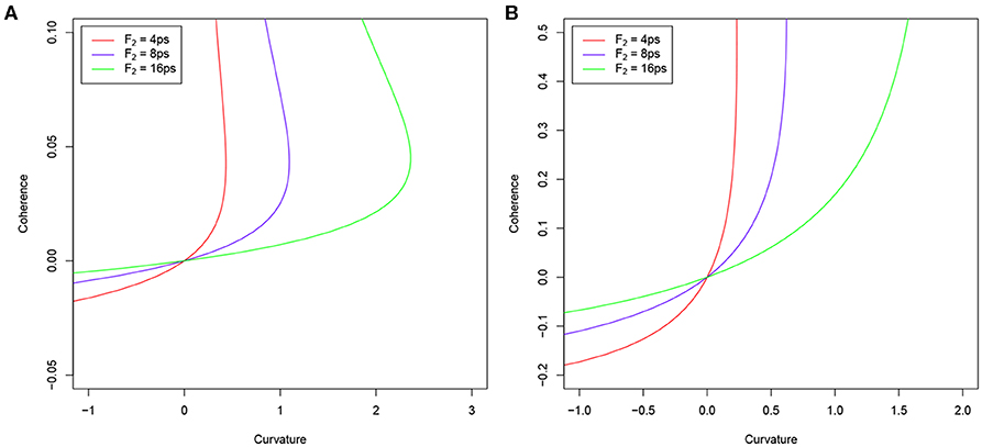
Figure 1. Coherence C(ρ) varies as the function of the curvature R. Red, Blue, and Green lines represent F2 = 4ps, F2 = 8ps, and F2 = 16ps, respectively. (A) Δε = ε1 − ε2 = 0.2ev and (B) Δε = ε1 − ε2 = 0.4ev. Other parameters are F1 = 2ps, T1 = 2100K, ε1 = 0.5ev, Δ = 0.3ev.
Therefore, quantum coherence is naturally connected to the internal curvature of the gauge field. Without quantum coherence, the gauge field is trivial associated with flat internal space. On the other hand, when the internal space is not flat and the gauge field is non-trivial, the detailed-balance is broken with non-local quantum coherence. This provides a new fundamental view in quantum physics: the non-local coherence can emerge from the non-equilibrium detailed-balance breaking which can be measured by an internal curvature of the gauge field in phase space.
The steady state curl quantum flux is of the form:
Here, from steady state curl quantum flux, we have the same observations as from the internal curvature Rμν discussed above.
On the other hand, from the coherent space {α, α*} to the Fock space, the coherence between αi and αj is equivalent to the coherence or coupling between eigenstate of different sites: |ni〉 and |nj〉, since the coherence is introduced by the interaction term . If the coupling between different sites vanishes, we have and no interactions between sites, which leads to the curvature Rμν → 0 and steady curl quantum flux . Therefore, there will be no quantum correlations regardless of the environmental conditions.
In this study, we have uncovered that non-equilibrium quantum dynamics gives rise to an intrinsic geometric curvature which can enhance quantum coherence. The non-equilibrium can be characterized by the curvature. This may help reveal an intrinsic connection between the space time geometry/topology and the quantum nature. On the one hand, curved space time may emerge from the non-equilibrium quantum dynamics, on the other hand, the intrinsic underlying curved space time may provide a possible channel (space time shortcut) or physical origin for the non-local quantum correlations such as coherence and entanglement. Furthermore, we illustrated that intrinsic curvature could lead to new fluctuation-dissipation theorem for non-equilibrium quantum systems. Therefore, the curved space time geometry/topology from non-equilibrium can give rise to new types of fluctuations in addition to the original spontaneous fluctuations. The non-equilibrium response is now linked not only to the spontaneous fluctuations around the equilibrium but also to the non-equilibrium fluctuations that originated from the curved geometry/topology or non-equilibrium. We have also shown that the curved geometry/topology characterized by the intrinsic curvature from non-equilibrium can generate quantum work and heat dissipation important for quantum thermodynamics. We believe our approach and results in the current study are general and can be applied to further study many interesting non-equilibrium quantum systems.
HF and JW have contributed to the organization, research performance, and writing of this article.
The authors declare that the research was conducted in the absence of any commercial or financial relationships that could be construed as a potential conflict of interest.
JW would like to acknowledge the support from the National Science Foundation PHY-76066.
The Supplementary Material for this article can be found online at: https://www.frontiersin.org/articles/10.3389/fphy.2020.00129/full#supplementary-material
1. Tao NJ. Electron transport in molecular junctions. Nat Nano. (2006) 1:173–81. doi: 10.1038/nnano.2006.130
2. Joachim C, Ratner MA. Molecular electronics: some views on transport junctions and beyond. Proc Natl Acad Sci USA. (2005) 102:8801–8. doi: 10.1073/pnas.0500075102
3. Nitzan A, Ratner MA. Electron transport in molecular wire junctions. Science. (2003) 300:1384–9. doi: 10.1126/science.1081572
4. Walter S, Nunnenkamp A, Bruder C. Quantum synchronization of a driven self-sustained oscillator. Phys Rev Lett. (2014) 112:094102. doi: 10.1103/PhysRevLett.112.094102
5. Ludwig M, Marquardt F. Quantum many-body dynamics in optomechanical arrays. Phys Rev Lett. (2013) 111:073603. doi: 10.1103/PhysRevLett.111.073603
6. Lee TE, Sadeghpour HR. Quantum synchronization of quantum van der Pol oscillators with trapped ions. Phys Rev Lett. (2013) 111:234101. doi: 10.1103/PhysRevLett.111.234101
7. Chen H, Wen X, Guo X, Zheng J. Intermolecular vibrational energy transfers in liquids and solids. Phys Chem Chem Phys. (2014) 16:13995. doi: 10.1039/C4CP01300J
8. Woutersen S, Bakker HJ. Resonant intermolecular transfer of vibrational energy in liquid water. Nature. (1999) 402:507–9. doi: 10.1038/990058
9. Zhang ZD, Wang J. Curl flux, coherence, and population landscape of molecular systems: nonequilibrium quantum steady state, energy (charge) transport, and thermodynamics. J Chem Phys. (2014) 140:245101. doi: 10.1063/1.4884125
10. Zhang ZD, Wang J. Assistance of Molecular Vibrations on Coherent Energy Transfer in Photosynthesis from the View of a Quantum Heat Engine. J Phys Chem B. (2015) 119:4662. doi: 10.1021/acs.jpcb.5b01569
11. Wang J, Xu L, Wang EK. Potential landscape and flux framework of nonequilibrium networks: robustness, dissipation, and coherence of biochemical oscillations. Proc Natl Acad Sci USA. (2008) 105:12271–6. doi: 10.1073/pnas.0800579105
12. Qian H. Open-system nonequilibrium steady state:? statistical thermodynamics, fluctuations, and chemical oscillations. J Phys Chem B. (2006) 110:15063–74. doi: 10.1021/jp061858z
13. Wang J. Landscape and flux theory of non-equilibrium dynamical systems with application to biology. Adv Phys. (2015) 64:1. doi: 10.1080/00018732.2015.1037068
14. Feng H, Wang J. Potential and flux decomposition for dynamical systems and non-equilibrium thermodynamics: curvature, gauge field, and generalized fluctuation-dissipation theorem. J Chem Phys. (2011) 135:234511. doi: 10.1063/1.3669448
15. Peskin ME, Schroeder DV. An Introduction to Quantum Field Theory. Addison-Wesley Publishing Company (1995).
16. Wigner EP. On the quantum correction for thermodynamic equilibrium. Phys Rev. (1932) 40:749. doi: 10.1103/PhysRev.40.749
17. Glauber RJ. Coherent and incoherent states of the radiation field. Phys Rev. (1963) 131:2766. doi: 10.1103/PhysRev.131.2766
18. Carmichael HJ. Statistical Methods in Quantum Optics 1: Master Equations and Fokker-Planck Equations. New York, NY: Springer (1999).
19. Zhang Z, Wu W, Wang J. Fluctuation-dissipation theorem for nonequilibrium quantum systems. Europhys Lett. (2016) 115:20004. doi: 10.1209/0295-5075/115/20004
20. Esposito M, Harbola U, Mukamel S. Nonequilibrium fluctuations, fluctuation theorems, and counting statistics in quantum systems. Rev Mod Phys. (2009) 81:1665. doi: 10.1103/RevModPhys.81.1665
21. Harbola U, Esposito M, Mukamel S. Quantum master equation for electron transport through quantum dots and single molecules. Phys Rev B. (2006) 74:235309. doi: 10.1103/PhysRevB.74.235309
22. Risken H. The Fokker-Planck Equation: Methods of Solution and Applications. Berlin: Springer-Verlag (1989).
23. Wang J, Zhang K, Wang E. Kinetic paths, time scale, and underlying landscapes: A path integral framework to study global natures of nonequilibrium systems and networks. J Chem Phys. (2010) 133:125103. doi: 10.1063/1.3478547
24. Evans DJ, Cohen EGD, Morriss GP. Probability of second law violations in shearing steady states. Phys Rev Lett. (1993) 71:2401–4. doi: 10.1103/PhysRevLett.71.2401
25. Evans DJ, Searles DJ. Equilibrium microstates which generate second law violating steady states. Phys Rev E. (1994) 50:1645–8. doi: 10.1103/PhysRevE.50.1645
26. Seifert U. Entropy production along a stochastic trajectory and an integral fluctuation theorem. Phys Rev Lett. (2005) 95:040602. doi: 10.1103/PhysRevLett.95.040602
27. Speck T, Seifert U. Integral fluctuation theorem for the housekeeping heat. J Phys A Math Gen. (2005) 38:L581. doi: 10.1088/0305-4470/38/34/L03
28. Kubo R. The fluctuation-dissipation theorem. Rep Prog Phys. (1966) 29:255–84. doi: 10.1088/0034-4885/29/1/306
29. Ruelle D. General linear response formula in statistical mechanics, and the fluctuation-dissipation theorem far from equilibrium. Phys Lett A. (1998) 245:220–4. doi: 10.1016/S0375-9601(98)00419-8
30. Colangeli M, Maes C, Wynants B. A meaningful expansion around detailed balance. J Phys A Math Theor. (2011) 44:095001. doi: 10.1088/1751-8113/44/9/095001
31. Marini Bettolo Marconi U, Puglisi A, Rondoni L, Vulpiani A. Fluctuation-dissipation: response theory in statistical physics. Phys Rep. (2008) 461:111. doi: 10.1016/j.physrep.2008.02.002
32. Deker U, Haake F. Fluctuation-dissipation theorems for classical processes. Phys Rev A. (1975) 11:2043. doi: 10.1103/PhysRevA.11.2043
33. Wang GM, Sevick EM, Mittag E, Searles DJ, Evans DJ. Experimental demonstration of violations of the second law of thermodynamics for small systems and short time scales. Phys Rev Lett. (2002) 89:050601. doi: 10.1103/PhysRevLett.89.050601
34. Andrieux D, Gaspard P. A fluctuation theorem for currents and non-linear response coefficients. J Stat Mech. (2007) P02006. doi: 10.1088/1742-5468/2007/02/P02006
35. Hummer G, Szabo A. Free energy reconstruction from nonequilibrium single-molecule pulling experiments. Proc Natl Acad Sci USA. (2001) 98:3658–61. doi: 10.1073/pnas.071034098
36. Jarzynski C. Nonequilibrium equality for free energy differences. Phys Rev Lett. (1997) 78:2690. doi: 10.1103/PhysRevLett.78.2690
Keywords: gauge field, non-equilibrium, coherence, quantum, geometric curvature
Citation: Feng H and Wang J (2020) The Quantum Coherence Induced by Geometric Curvature of Gauge Field in Non-equilibrium Quantum Dynamics. Front. Phys. 8:129. doi: 10.3389/fphy.2020.00129
Received: 12 December 2019; Accepted: 03 April 2020;
Published: 13 May 2020.
Edited by:
Fernando A. Oliveira, University of Brasilia, BrazilReviewed by:
Carmine Ortix, University of Salerno, ItalyCopyright © 2020 Feng and Wang. This is an open-access article distributed under the terms of the Creative Commons Attribution License (CC BY). The use, distribution or reproduction in other forums is permitted, provided the original author(s) and the copyright owner(s) are credited and that the original publication in this journal is cited, in accordance with accepted academic practice. No use, distribution or reproduction is permitted which does not comply with these terms.
*Correspondence: Jin Wang, amluLndhbmcuMUBzdG9ueWJyb29rLmVkdQ==
Disclaimer: All claims expressed in this article are solely those of the authors and do not necessarily represent those of their affiliated organizations, or those of the publisher, the editors and the reviewers. Any product that may be evaluated in this article or claim that may be made by its manufacturer is not guaranteed or endorsed by the publisher.
Research integrity at Frontiers
Learn more about the work of our research integrity team to safeguard the quality of each article we publish.