Discrete Geometrical Invariants in 3D Space: How Three Random Sequences Can Be Compared in Terms of “Universal” Statistical Parameters

Previous work has determined the discrete geometrical invariant (DGI) in 2D space, which allows the analysis of a pair of random sequences ([r_1k, r_2k], k = 1,2,…N) containing an equal number of data points to be reduced to eight “universal” parameters that present different inter-correlations between the two compared sequences. These eight parameters can serve as a “universal” platform for comparison of various random sequences of different natures. In this paper, we derive mathematical expressions for the DGI in 3D space, which represent three random sequences in the form of a “trajectory” of an “imaginary” particle in 3D space. The DGI is of the fourth order in 3D space and allows three random sequences ({r_1k, r_2k, r_3k}, k = 1,2,…N) to be compared with one another. This unified and “universal” platform identifies (in total) six surfaces and 13 reduced and compact parameters obtained from 28 basic moments and their intercorrelations up to the fourth order, inclusively. The transcendental numbers π and E (Euler constant) are considered as examples of the use of the DGI method, and their 3D images are derived together with values for the 13 quantitative parameters that differentiate them from each other. An application of the method, identifying two different classes of earthquake data, is also presented to illustrate the potentially wide application of the approach to the identification and classification of nominally random data sequences.

Introduction and Formulation of the Problem

The statement that any random sequence has a set of deterministic components sounds absurd and unacceptable. In fact, many researchers claim that one can find true irreproducible random sequences that cannot be compared or correlated with each other, basing their claim on the theory of dynamic chaos. This statement is especially important in modern cryptography, where the search for cryptographically stable codes remains a real problem [1–3]. From a different point of view, however, it is important to find fitting functions for complex systems, where the “best fit” model function is absent. Any fitting function intended to provide a quantitative description of a given set of data must be expressed in an analytical form and hence can be considered a deterministic function. Such a function can be used to fit a given set of random data, implying the ability to construct a neuro-net and make predictions for the continuation of the data sequence. In [4, 5], for example, a “universal” fitting function was found that represented a segment of the Prony series that can be used for the fitting of data associated with any quasi-reproducible experiment. For non-reproducible experiments, one can use the NAFASS (Nonorthogonal Amplitude-Frequency Analysis of the Smoothed Signals) approach [6, 7]. There is therefore something of a contradiction: some researchers claim that it is impossible to find a fitting function for “true” random sequences, but on the other hand, research is carried out to find the desired fitting function for complex systems, where the “best fit” function is absent. Recently [8, 9], however, it has been shown that the ideas expressed in the generalization of the Pythagorean theorem proposed by Babenko [10, 11], which was proved for 2D and 3D figures with different symmetry, can be developed to take into consideration different random sequences. In this way, a 2D approach has allowed real data for different types of olive oils to be compared [8] and Weierstrass-Mandelbrot sequences to be compared together with other real data, such that the differences between them could be expressed in terms of different inter-correlations up to the fourth order, inclusively [9]. The approach is reminiscent of the universal form of the partition function proposed by Gibbs in classical/quantum statistical mechanics, where all microscopic parameters are transformed to a finite and compact set of thermodynamic variables. A similar formulation for a pair of random sequences belonging to 2D space is realized with the help of a discrete geometrical invariant (DGI).

Here we intend to extend the approach of [8, 9] to prove that the compact form of the discrete geometrical invariant (DGI) of the fourth order also exists in 3D space. This surface is of the fourth order and admits the separation of random sequences in a spherical coordinate system that allows the surface to be expressed in analytical and visual form. The DGI that we obtain plays a similar role to the partition function in statistical physics by allowing the transformation of 3N random data points into a 13D indication space. We think that the reduced number of 13 parameters (incorporating in itself 28 moments and different intercorrelations up to the fourth order, inclusive) is sufficient for classification of the variety of random sequences in 3D space. Furthermore, the DGI of the fourth order that has been obtained can be expressed in the form of six surfaces in the 3D space. These 3D-images facilitate the analysis and classification of different random sequences of various natures. The main outcome of this approach is that it creates a “universal” platform for the classification of different random sequences in one scheme described by the set of 13 (28) unified parameters.

Description of the Algorithm and Basic Formulas

In this section, we present the necessary “algebra” for derivation of the desired DGI of the fourth order in 3D space including three random sequences ({r_1k, r_2k, r_3k} k = 1,2,…N).

We start from the fourth-order expression:

$\begin{array}{ll}\begin{array}{c}{L}_k^{(4)}=A_{40}^{(1,0)}{(y_1-r_{1k})}^4+A_{40}^{(2,0)}{(y_2-r_{2k})}^4\hfill \\ +A_{40}^{(3,0)}{(y_3-r_{3k})}^4-\hfill \\ -2B_{22}^{(1,2)}{(y_1-r_{1k})}^2{(y_2-r_{2k})}^2\hfill \\ -2B_{22}^{(1,3)}{(y_1-r_{1k})}^2{(y_3-r_{3k})}^2-\hfill \\ -2B_{22}^{(2,3)}{(y_2-r_{2k})}^2{(y_3-r_{3k})}^2\hfill \\ +C_{2,1,1}^{1(2,3)}{(y_1-r_{1k})}^2(y_2-r_{2k})(y_3-r_{3k})+\hfill \\ +C_{2,1,1}^{2(1,3)}{(y_2-r_{2k})}^2(y_1-r_{1k})(y_3-r_{3k})\hfill \\ +C_{2,1,1}^{3(1,2)}{(y_3-r_{3k})}^2(y_1-r_{1k})(y_2-r_{2k}).\hfill \end{array}\hfill & (1)\end{array}$

Here, the upper indices of the coefficients of the right-hand side indicate an arbitrary point M(y₁, y₂, y₃) in the 3D space and its order, having three arbitrary Cartesian coordinates (y₁, y₂, y₃) combined with the same number of random sequences r_ik, (i = 1,2,3). The lower indices indicate the corresponding power-law exponents. This set of combinations is not complete; we omit the combinations $D_{3,1}^{(1,2)},D_{3,1}^{(1,3)},D_{3,1}^{(2,3)}$ in order not to increase the number of additional parameters too much. As necessary, these three combinations can be imbedded into expression (1) or can be considered separately. The calculations given below show that there are in total 28 different parameters that incorporate: 3 first moments, 6 second moments and their pair correlations, 10 third moments and their inter-correlations and, finally, 9 moments of the fourth order and their correlations. As will be shown below, these parameters can be unified into 13 compact parameters that are sufficient for analysis and classification of three basic random sequences having 3N data points initially. We propose that this reduced 13D indication space is sufficient for many practical purposes.

The desired fourth order invariant is obtained from the formula:

$\begin{array}{ll}\frac{1}{N}{\displaystyle \sum _{k=1}^N}{L}_k^{(4)}=I.& (2)\end{array}$

In order to decrease the number of parameters and obtain a compact expression that does not depend on them, we use the condition that all linear terms in expression (2) are equal to zero. This condition allows the desired invariant to be found in the compact form and the realization of the reduction procedure of 10 moments and inter-correlations of the third order to three combinations only. If one avoids this condition, the desired invariant loses its closed form. Besides, this requirement allows three conditions between parameters $A_{40}^{(1,0)},A_{40}^{(2,0)},A_{40}^{(3,0)};B_{22}^{(1,2)},B_{22}^{(1,3)},B_{22}^{(2,3)},C_{2,1,1}^{1(2,3)},C_{2,1,1}^{2(1,3)},C_{2,1,1}^{3(1,2)}$ to be found in the form of three ratios:

$\begin{array}{ll}\begin{array}{c}{A}_{40}^{(1,0)}=A_{40}^{(2,0)}=A_{40}^{(3,0)}\equiv A,\hfill \\ R^{(1,2)}=\frac{B_{22}^{(1,2)}}{A}=\frac{C_{2,1,1}^{3(1,2)}}{A};\hfill \\ R^{(1,3)}=\frac{B_{22}^{(1,3)}}{A}=\frac{C_{2,1,1}^{2(1,3)}}{A};R^{(2,3)}=\frac{B_{22}^{(2,3)}}{A}=\frac{C_{2,1,1}^{1(2,3)}}{A}.\hfill \end{array}\hfill & (3)\end{array}$

The ratios R^{(1, 2)}, R^{(1, 3)}, and R^{(2, 3)}, which play an important role in this work, satisfy the linear system of algebraic equations:

$\begin{array}{ll}\begin{array}{c}\left[4Q_{122}-Q_{233}\right]·R^{(1,2)}+\left[4Q_{133}-Q_{223}\right]\hfill \\ ·R^{(1,3)}-2Q_{123}·R^{(2,3)}=4Q_{111}\hfill \\ \left[4Q_{112}-Q_{133}\right]·R^{(1,2)}-2Q_{123}·R^{(1,3)}\hfill \\ +\left[4Q_{233}-Q_{113}\right]·R^{(2,3)}=4Q_{222}\hfill \\ -2Q_{123}·R^{(1,2)}+\left[4Q_{113}-Q_{122}\right]·R^{(1,3)}\hfill \\ +\left[4Q_{223}-Q_{113}\right]·R^{(2,3)}=4Q_{333}\hfill \end{array}\hfill & (4)\end{array}$

Here, we introduce the following definitions for the 10 correlations of the third order:

$\begin{array}{ll}\begin{array}{c}{Q}_{\alpha \beta \gamma }=\frac{1}{N}{\displaystyle \sum _{k=1}^N}(r_{\alpha k}-\langle r_{\alpha }\rangle )·(r_{\beta k}-\langle r_{\beta }\rangle )·(r_{\gamma k}-\langle r_{\gamma }\rangle )\equiv \hfill \\ \equiv \langle \Delta r_{\alpha }\Delta r_{\beta }\Delta r_{\gamma }\rangle ,\alpha ,\beta ,\gamma =1,2,3.\hfill \end{array}\hfill & (5)\end{array}$

We do not give the solutions of equation (4) in the explicit form because the final expressions look cumbersome. The equation system (4) plays a key role in the construction of the desired invariant because it allows 10 correlations of the third order to be reduced to three basic correlation parameters R^{(1, 2)}, R^{(1, 3)}, and R^{(2, 3)}. It is interesting to realize their symmetrical properties relative to the input random sequences. If all three compared sequences coincide with each other (r_1k = r_2k = r_3k, k = 1,2,…N), then R^{(1, 2)} = R^{(1, 3)} = R^{(2, 3)} = R, and solving (4) gives R = 1 (the case of spherical symmetry). If only two sequences coincide with each other, r_1k = r_2k ≠ r_3k, i.e., the case of cylindrical symmetry, the coupled linear system (4) is reduced to a couple of linear equations relative to the variables R^{(1, 2)} ≠ R^{(1, 3)} = R^{(2, 3)}. The number of triple correlations equals four in this case (Q₁₁₁, Q₁₁₃, Q₁₃₃, Q₃₃₃).

$\begin{array}{ll}\begin{array}{c}\left[4Q_{111}-Q_{133}\right]·R^{(1,2)}+\left[4Q_{133}-3Q_{113}\right]·R^{(1,3)}=4Q_{111}\hfill \\ -2Q_{123}·R^{(1,2)}+2\left[4Q_{113}-Q_{111}\right]·R^{(1,3)}=4Q_{333}\hfill \end{array}\hfill & (6)\end{array}$

The two unknown parameters R^{(1, 2)}, R^{(1, 3)} from (6) can be expressed in an explicit form.

After all average transformations are made in expression (2), the final expression for the DGI in 3D space takes the form:

$\begin{array}{ll}{K}_4(Y_1,Y_2,Y_3)+K_2(Y_1,Y_2,Y_3)=I& (7)\end{array}$

This equation describes a 3D surface in terms of relative variables, Y₁, Y₂, Y₃. As in Nigmatullin and Vorobev [9] and Babenko [10], we note that the expression for the constant I is found from the condition that 2I is a constant expression including all quadruple correlations figuring in the left-hand side. This condition leads to the following expression for I:

$\begin{array}{ll}\begin{array}{c}I=Q_{1111}+Q_{2222}+Q_{3333}+R^{(1,2)}(Q_{3312}-2Q_{1122})+\hfill \\ +R^{(1,3)}(Q_{2213}-2Q_{1133})+R^{(2,3)}(Q_{1123}-2Q_{2233}).\hfill \end{array}\hfill & (8)\end{array}$

Here the correlations of the fourth order can be presented in the following compact form:

$\begin{array}{ll}\begin{array}{c}{Q}_{\alpha \beta \gamma \delta }=\frac{1}{N}{\displaystyle \sum _{k=1}^N}(r_{\alpha k}-\langle r_{\alpha }\rangle )·(r_{\beta k}-\langle r_{\beta }\rangle )·(r_{\gamma k}-\langle r_{\gamma }\rangle )\hfill \\ ·(r_{\delta k}-\langle r_{\delta }\rangle )\equiv \hfill \\ \equiv \langle \Delta r_{\alpha }\Delta r_{\beta }\Delta r_{\gamma }\Delta r_{\delta }\rangle ,\alpha ,\beta ,\gamma ,\delta =1,2,3.\hfill \end{array}\hfill & (9)\end{array}$

After simple algebraic transformations, the fourth order term K₄(Y₁, Y₂, Y₃) figuring in (7) can be expressed as:

$\begin{array}{ll}\begin{array}{c}{K}_4(Y_1,Y_2,Y_3)={\displaystyle \sum _{i=1}^3}{Y}_i^4+R^{(1,2)}(Y_3^2·Y_1·Y_2-2Y_1^2{Y}_2^2)+\hfill \\ +R^{(1,3)}(Y_2^2·Y_1·Y_3-2Y_1^2{Y}_3^2)\hfill \\ +R^{(2,3)}(Y_1^2·Y_2·Y_3-2Y_2^2{Y}_3^2).\hfill \end{array}\hfill & (10)\end{array}$

The coefficients R^{(1, 2)}, R^{(1, 3)}, R^{(2, 3)} are found from equation system (4). The variables Y_{1, 2, 3} defining the coordinates of the unknown point M (Y₁, Y₂, Y₃) relative to the gravity center of the random sequences are expressed as:

$\begin{array}{ll}{Y}_i=y_i-\langle r_i\rangle ,\langle r_i\rangle =\frac{1}{N}{\displaystyle \sum _{k=1}^N}{r}_{ik}.& (11)\end{array}$

The complete quadratic form figuring in (7) can be written as:

$\begin{array}{ll}{K}_2(Y_1,Y_2,Y_3)={\displaystyle \sum _{\alpha <\beta =1}^3}{M}_{\alpha \beta }{Y}_{\alpha }{Y}_{\beta }.& (12)\end{array}$

The six matrix coefficients M_αβ mixing the correlations of the second and third orders, accordingly, can be presented as:

$\begin{array}{ll}\begin{array}{c}{M}_{11}=6Q_{11}-2Q_{22}{R}^{(1,2)}-2Q_{33}{R}^{(1,3)}+Q_{23}{R}^{(2,3)},\hfill \\ M_{22}=6Q_{22}-2Q_{11}{R}^{(1,2)}+Q_{13}{R}^{(1,3)}-2Q_{33}{R}^{(2,3)},\hfill \\ M_{33}=6Q_{33}+Q_{12}{R}^{(1,2)}-2Q_{11}{R}^{(1,3)}-2Q_{22}{R}^{(2,3)},\hfill \\ M_{12}=(-8Q_{12}+Q_{33})R^{(1,2)}+2Q_{12}{R}^{(1,3)}+2Q_{13}{R}^{(2,3)},\hfill \\ M_{13}=2Q_{23}{R}^{(1,2)}+(-8Q_{13}+Q_{22})R^{(1,3)}+2Q_{12}{R}^{(2,3)},\hfill \\ M_{23}=2Q_{13}{R}^{(1,2)}+2Q_{23}{R}^{(1,3)}+(-8Q_{23}+Q_{11})R^{(2,3)}.\hfill \end{array}\hfill & (13)\end{array}$

The constraints defined by equation set (4) allow the surface (7) to be separated into spherical coordinates when it is written relative to the initial variables Y_{1, 2, 3}. Introducing the notations

$\begin{array}{ll}\begin{array}{c}{y}_1=\langle r_1\rangle +R(\phi ,\theta )\text{cos}(\phi )\text{sin}(\theta ),\hfill \\ y_2=\langle r_2\rangle +R(\phi ,\theta )\text{sin}(\phi )\text{sin}(\theta ),\hfill \\ y_3=\langle r_3\rangle +R(\phi ,\theta )\text{cos}(\theta ),\hfill \\ 0\le \phi <2\pi ,0\le \theta <\pi ,R\ge 0,\hfill \end{array}\hfill & (14)\end{array}$

and then inserting these variables into expression (7), one can obtain the equation for the radial distance R(φ, θ):

$\begin{array}{ll}{R}^4(\phi ,\theta )P_4(\phi ,\theta )+R^2(\phi ,\theta )P_2(\phi ,\theta )=I& (15)\end{array}$

From equation (15), it is easy to find the positive root for the desired radial distance R(φ, θ):

$\begin{array}{ll}R(\phi ,\theta )={\left[\frac{\sqrt{P_2^2(\phi ,\theta )+4I·P_4(\phi ,\theta )}-P_2(\phi ,\theta )}{2·P_4(\phi ,\theta )}\right]}^{1/2}& (16)\end{array}$

The polynomials P_{2, 4}(φ, θ) in equations (15) and (16) are defined by the following expressions:

$\begin{array}{l}{P}_4(\phi )={\cos }^4(\phi ){\sin }^4\left(\text{θ}\right)+{\sin }^4(\phi ){\sin }^4\left(\text{θ}\right)\\ +{\cos }^4\left(\text{θ}\right)+\\ +R^{(1,2)}[\sin (\phi )\cos (\phi ){\sin }^2\left(\text{θ}\right){\cos }^2\left(\text{θ}\right)\\ -2·{\sin }^2(\phi ){\cos }^2(\phi ){\sin }^4\left(\text{θ}\right)]+\\ +R^{(1,3)}[{\sin }^2(\phi )\cos (\phi ){\sin }^3\left(\text{θ}\right)\cos \left(\text{θ}\right)\\ -2·{\cos }^2(\phi ){\sin }^2\left(\text{θ}\right){\cos }^2\left(\text{θ}\right)]+\\ +R^{(2,3)}[\sin (\phi ){\cos }^2(\phi ){\sin }^3\left(\text{θ}\right)\cos \left(\text{θ}\right)\\ -2·{\sin }^2(\phi ){\sin }^2\left(\text{θ}\right){\cos }^2\left(\text{θ}\right)].& (\mathrm{17a})\end{array}$

$\begin{array}{ll}\begin{array}{c}{P}_2(\phi ,\theta )=M_{11}{\text{cos}}^2(\phi ){\text{sin}}^2(\theta )+M_{22}{\text{sin}}^2(\phi ){\text{sin}}^2(\theta )\hfill \\ +M_{33}{\text{cos}}^2(\theta )+\hfill \\ +M_{12}\text{sin}(\phi )\text{cos}(\phi ){\text{sin}}^2(\theta )\hfill \\ +M_{13}\text{cos}(\phi )\text{sin}(\theta )\text{cos}(\theta )\hfill \\ +M_{23}\text{sin}(\phi )\text{sin}(\theta )\text{cos}(\theta ).\hfill \end{array}\hfill & (\mathrm{17b})\end{array}$

Here the matrix parameters M_αβ (α,β = 1,2,3) are defined by (13).

Expressions (14), (16), and (17) completely determine the desired DGI in 3D space. There are other DGIs admitting the existence of other variables associated with the constants, $D_{3,1}^{(1,2)},D_{3,1}^{(1,3)},D_{3,1}^{(2,3)}$, that we have omitted here. However, we stress that only the nullification of the linear terms allows structure (7) to be constructed, which leads finally to the closed parameterization of type (14), which includes other combinations of spherical polynomials P_{2, 4}(φ, θ). When the cubic and linear terms are included in the invariant of the fourth order (2), the closed structure of equation (14) cannot be constructed in the compact form. Concluding this section, we should stress that one has three surfaces (14); however, expression (16) admits the existence of a solution when the radicand becomes negative. It corresponds to the condition I < 0 in expression (16). In this case, in addition to expression (14), one can have three additional 3D surfaces:

$\begin{array}{ll}\begin{array}{c}{Y}_1=\text{Im}(R(\phi ,\theta ))\text{cos}(\phi )\text{sin}(\theta ),\hfill \\ Y_2=\text{Im}(R(\phi ,\theta ))\text{sin}(\phi )\text{sin}(\theta ),\hfill \\ Y_3=\text{Im}(R(\phi ,\theta ))\text{cos}(\theta )\hfill \\ 0\le \phi <2\pi ,0\le \theta <\pi ,R\ge 0,\text{Im}(R(\phi ,\theta ))>0.\hfill \end{array}\hfill & (18)\end{array}$

Expression (18) will be helpful also in cases where it is necessary to have an additional source of information for separation of the given random sequences from each other. If this information is redundant and not necessary, one can consider only the modulus of the radial distance $|R(\phi ,\theta )|=\sqrt{Re{(R(\phi ,\theta ))}^2+Im{(R(\phi ,\theta ))}^2}$. In this paper, in order to decrease the number of figures, we consider only expression (14), having in mind only the real part of the radial distance R(φ, θ).

Application the DGI method for differentiation of the trans-numbers π and E

In order not to overload this paper with a large number of figures, we consider the 3D structure of two famous transcendental numbers: (a) π = 3.141492653689793238462643…and (b) Euler constant E = 2.718281828459045235360287…. Each of these numbers containing 60,000 data points is combined into a set of normalized triads. These 20,000 triads are transformed to an “ideal” noise in accordance with the following procedure: (a) the integer part is omitted; (b) each three digits of the infinite sequence form a normalized number in the interval [0,1] after division by 1,000. For example, the number of π forms the following sequence of numbers falling into the interval [0,1]. π = 3.141 492 653 689 793 238 462 643 → 0.141, 0.492, 0.653, 0.689, 0.793, 0.238, 0.462, 0.643,… Normalized triads for E are obtained similarly. Then we apply the procedure of reduction to three incident points. This procedure is described in previous papers [12, 13]. It allows three types of noise to be obtained from a sequence, i.e., sequences of group-localized maximal [Yup(x)], minimal [Ydn(x)], and mean values [Ymn(x)], correspondingly. After application of the reduction procedure to three incident points (the compression parameter b = 20, i.e., we compress twenty points in the sequence to their mean, maximum, and minimum values), each local set {b₁, b₂,…, b₂₀} is reduced to three incident points {max(b), min(b), and mean(b)}, giving the desired three sequences. We want to stress also that these three remarkable points are invariant relative to all possible permutations inside the chosen local set {b}. They are shown for the trans-number π in Figure 1 and contain 1,000 data points only. Relationship (14), as a “fingerprint,” gives three surfaces for the real part of the radial distance R(φ, θ), and, similarly, it can contain three additional surfaces for the imaginary part of the radial distance, implying that Im R(φ, θ) > 0, when the radicand in (16) becomes negative. As has been mentioned above, we omit these surfaces for simplicity. Finally, for the identification of the chosen trans-number π, we have three 3D surfaces and a minimum number of 13 parameters (three parameters identify the gravity center < r_i> (i = 1,2,3), three parameters R^{(1, 2), (1, 3), (2, 3)} associated with the reduced triple correlations calculated from the linear system (4), six parameters from (13) identifying the correlation of the second order, and, finally, the value of the invariant I from relationship (8). This 13D indication and reduced space is in most cases sufficient for finding the differences between compared random sequences. In Figures 2–4, we show the three desired surfaces corresponding to trans-number π for the real values of the radial distance R(φ,θ) > 0. The 13 parameters identifying these surfaces are given in Table 1. Similarly, we realize the same procedure for E (see Figures 5–8 for details). The comparison of the reduced parameters given in Table 1 for the two trans-numbers clearly demonstrates their difference. These differences are seen in the values of the parameters and even in their signs. It is not yet clear which parameter is the most sensitive to a possible perturbation (possible attack of the given “ideal” noise). The analysis of these possible perturbations form the subject of further work.

FIGURE 1

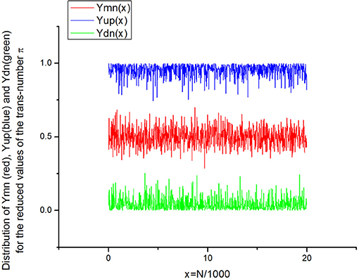
Figure 1. Three distributions of the “ideal” noise obtained for the transcendental number π. They are compressed by the factor b = 20 and contain only 1,000 data points. They form three initial random sequences that can be transformed into three 3D-surfaces for identification of their differences and formation of a specific “fingerprint”.

FIGURE 2

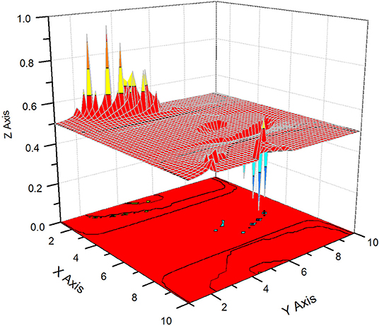
Figure 2. This is the first 3D surface formed by the curve y₁(φ,θ). The scale for the angles φ [OX axis] and θ [OY axis] is given in the discrete numbers of the visible data points. Each angle is digitized as φ_j = 2π·(j/10), θ_j = π·(j/10), and j = 0,1,…,10.

FIGURE 3

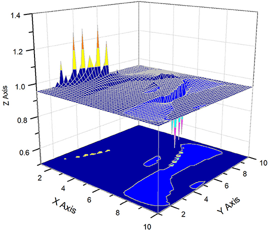
Figure 3. Here we display the surface formed by the curve y₂(φ,θ). The scale for the angles φ [OX axis] and θ OY axis] is given in the numbers corresponding to the discrete data points (j = 0,1,..10).

FIGURE 4

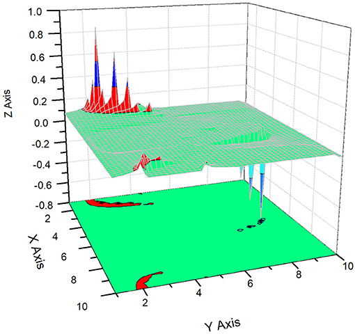
Figure 4. Here we display the surface formed by the curve y₃(φ,θ). The scale is similar to that of the previous figures.

TABLE 1

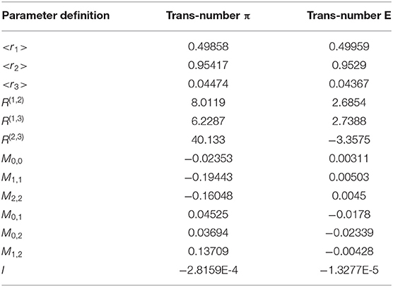
Table 1. The comparison of the 13 basic parameters that correspond to the trans-numbers π and E.

FIGURE 5

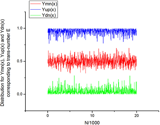
Figure 5. Three distributions of the initial “ideal” noise obtained for the transcendental number E, with the initial sequence compressed by the factor b = 20 and containing only 1,000 data points. They form three initial random sequences that can be transformed into three 3D-surfaces for identification of their differences and formation of a specific “fingerprint.” Visually, this noise looks like the “ideal” noise depicted in Figure 1.

FIGURE 6

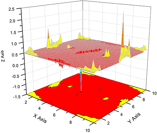
Figure 6. This figure corresponds to the surface Z = y₁(φ,θ) for the trans-number E. The scale for the angles φ [OX axis] and θ [OY axis] is given in the numbers of the visible data points. Each angle is digitized as X Axis = φ_j = 2π·(j/10), Y Axis = θ_j = π·(j/10), j = 0,1,…,10.

FIGURE 7

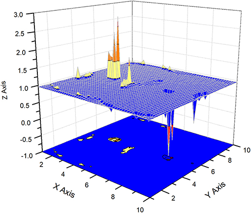
Figure 7. This figure corresponds to the surface Z = y₂(φ,θ) for the trans-number E. The scale for the angles φ [OX axis] and θ [OY axis] is kept the same. Each angle is digitized as X Axis = φ_j = 2π·(j/10), Y Axis = θ_j = π·(j/10), j = 0,1,…,10. This figure should be compared with Figure 3, where the same surface Z=y₂(φ,θ) for the trans-number π is shown.

FIGURE 8

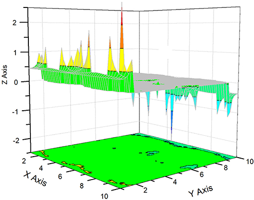
Figure 8. Here we display the surface formed by the curve y₃(φ,θ). The scale and axes notations are similar to previous figures.

DGI Analysis of Earthquake (EQ) Signals

Close analysis of the method we have proposed allows a simplified version of the DGI presentation to be obtained, where by applying a similar digitization to the corresponding angles φ_j = 2π·j/N and θ_j = π·j/N (j = 0,1,…, N), we obtain specific “projections” of all three surfaces onto the plane j/N. In this case, we have three deterministic curves y_{1, 2, 3}(j) that are defined as:

$\begin{array}{ll}\begin{array}{c}{y}_1(j)=\langle r_1\rangle +R({\phi }_j,{\theta }_j)\text{cos}({\phi }_j)\text{sin}({\theta }_j),\hfill \\ y_2(j)=\langle r_2\rangle +R({\phi }_j,{\theta }_j)\text{sin}({\phi }_j)\text{sin}({\theta }_j),\hfill \\ y_3(j)=\langle r_3\rangle +R({\phi }_j,{\theta }_j)\text{cos}({\theta }_j),\hfill \\ {\phi }_j=2\pi \left(\frac{j}{N}\right),\theta =\pi \left(\frac{j}{N}\right),R_j\ge 0,j=0.1\dots ,N.\hfill \end{array}\hfill & (19)\end{array}$

These three functions can serve for identification and quantitative description of the given random/deterministic sequences. The compact number of parameters that determine the behavior remains the same and is equal to 13. The authors decided to apply this simplified analysis to the differentiation and recognition of available EQ data. It is known that the direct quantitative description of EQ perturbations itself represents an unsolved and complex problem. Recently, one of us (RRN), together with other geophysicists, was able to apply the NAFASS approach for describing the envelopes of a set of EQs [14]. However, in many cases, it is not sufficient. It is desirable to have a unified quantitative platform that enables a comparison of various EQs recorded from different sources. The approach proposed here can serve as a promising tool for the solution of this problem. Referring a potential reader to the reference [14], the authors decided to compare six randomly taken EQ signals recorded from one source (selected EQ signals were obtained from Karagay Bulak station, the Kyrgyz Republic). We are not going to consider this problem in detail, as, for us, it is important only to demonstrate the possibility of applying the DGI approach [expressed in its simplest form (19)] to this complex phenomenon as a quantitative description and possible classification of the complex EQ signals.

The applied algorithm remains partly the same as was used for the trans-numbers above. We reduced the chosen EQ signal to three signals, again selecting their sequences {in terms of the localized maximal [Yup(x)], mean [Ymn(x)], and minimal [Ydn(x)] values}, correspondingly. The compression factor b = 5. A typical triple EQ signal compressed by a factor of five is shown in Figure 9. Application of expressions (19) allows the desired y_{1, 2, 3}(j) projections (j = 1,2,…N = 50) to be calculated. These three functions, associated with specific projections of three surfaces on the common plane, can be considered to be the quantitative identifiers of the given EQ-1 signal. These function-projections are shown in Figure 10. Similarly, one can calculate other EQ signals (2–6). Their corresponding projection functions, together with their signals, are depicted in Figures 11–15, and their parameters are collected in Table 2. Preliminary analysis of these figures allows it to be concluded that the functions y_{1, 2, 3}(j) for the EQs-1, 3, 4, 6 have the same statistical nature. The other two EQs-2, 5, are different and should be analyzed separately. Therefore, even the simplified version of the DGI approach, realized in a planar projection, allows a naive user (i.e., one not having any specialized geophysical education) to differentiate the EQs and select those that are similar with close statistical characteristics. It implies that this routine work can be realized with the help of a computer program containing the DGI algorithm.

FIGURE 9

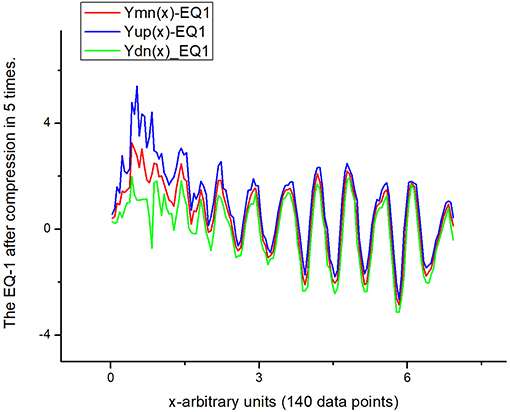
Figure 9. The recorded signal corresponding to the EQ-1. After compression by a factor of 5 (b = 5) the reduced signal contains 140 data points only.

FIGURE 10

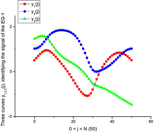
Figure 10. Three curves y_{1, 2, 3}(j) that were calculated with the help of expression (19) and correspond to the EQ-1 signal in 3D—DGI projection space. All 13 quantitative parameters are collected in Table 2.

FIGURE 11

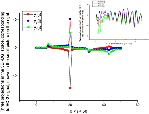
Figure 11. Three curves corresponding to the projections of the EQ-2 signal. As one can notice this signal is different to the signal shown in Figure 9. Therefore, the usage of the y_{1, 2, 3}(j) projections helps to differentiate them, at least qualitatively.

FIGURE 12

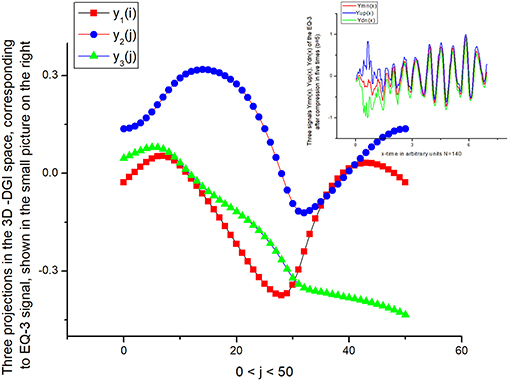
Figure 12. Comparison of this figure with Figure 10 allows a preliminary conclusion about the statistical similarity of the EQ-1 with EQ-3 to be made, i.e., the corresponding projections y_{1, 2, 3}(j) are very similar to each other.

FIGURE 13

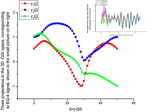
Figure 13. Plots for y_{1, 2, 3}(j) of the EQ-4 signal. In spite of their quantitative difference the EQs-1, 3, 4 have the same statistical nature.

FIGURE 14

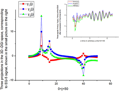
Figure 14. The projections y_{1, 2, 3}(j) of the EQ-5 have quite different behavior to those of EQ-1, 3, 4, 6, and the nature of this signal should be analyzed separately.

FIGURE 15

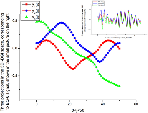
Figure 15. The behavior of these projections y_{1, 2, 3}(j) corresponding to EQ-6 are, in spite of their differences in amplitudes, similar to EQs-1,3,4. Therefore, this analysis of the different EQs enables them to be classified as similar or different.

TABLE 2

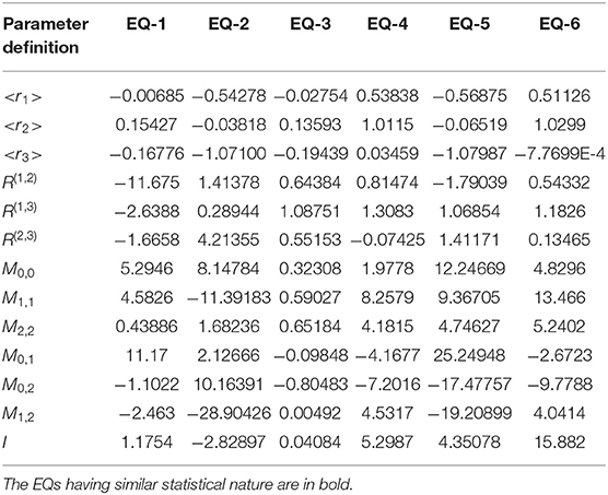
Table 2. The comparison of the 13 basic parameters that correspond to the EQs-1–6.

Discussion and Conclusions

In this paper, the authors propose an extension of the DGI approach realized previously for 2D space. It allows the comparison of three random sequences characterizing a complex object (having, in general, a 3D structure) and the transformation of it into six surfaces for its reliable identification and classification with other objects. Each surface has 13 compact parameters (derived from 28 moments and their inter-correlations), that allow it to be used as a general platform for the comparison of different random or deterministic sequences. We stress again that the DGI transformation is similar to the partition function used in the statistical mechanics. The same compression of the 3N data points initially present in the given sequences by the proposed DGI approach derived for 3D space allows them to be transformed to 13 (28) statistical parameters for their quantitative description.

Examples, associated with the classification of the famous transcendental numbers π and E and randomly taken EQ signals, have been presented in order to convince a skeptical reader to approach this work from a wide perspective and to see in it a general method that will undoubtedly find a wide field of application in the solution of different problems associated with the quantitative analysis of different random and even deterministic functions. The framework of the paper does not allow the authors to present other interesting possibilities for the proposed DGI method. They do hope that potential researchers will quickly understand its nature and potential power for application in the natural sciences and modern engineering.

Data Availability Statement

The datasets generated for this study are available on request to the corresponding author.

Author Contributions

The author confirms being the sole contributor of this work and has approved it for publication.

Conflict of Interest

The author declares that the research was conducted in the absence of any commercial or financial relationships that could be construed as a potential conflict of interest.

Acknowledgments

RN expresses his thanks to Dr. Ksenia Nepeina (Karagay Bulak station, Kyrgyzstan Republic) for providing the possibility of using the EQ data considered in this analysis. The author expresses deep thanks for Dr. Prof. Len Dissado for attentive reading the previous version of a manuscript and help in writing the final chapter.

References

1. Aumasson J-P. Serious Cryptography, A Practical Introduction to Modern Encryption. San-Francisco, CA: No Starch Press. (2018).

Google Scholar

2. Scneier B. Secrets & Lies, Digital Security in a Network World. New York, NY: John Wiley &Sons, Inc. (2000).

Google Scholar

3. Menezes A, van-Oorschot P, Vanstone S. Handbook of Applied Cryptography. Boca Raton, FL: CRC Press (1996).

Google Scholar

4. Nigmatullin RR, Maione G, Lino P, Saponaro F, Zhang W. The general theory of the quasi-reproducible experiments: How to describe the measured data of complex systems? Commun Nonlinear Sci Num Simul. (2017) 42:324–41. doi: 10.1016/j.cnsns.2016.05.019

CrossRef Full Text | Google Scholar

5. Nigmatullin RR. Detection of quasi-periodic processes in experimental measurements: reduction to an “ideal experiment” Chapter 1. In: Luo A, Afraimovich V, Machado JAT, Zhang J, editors. Complex Motions and Chaos in Nonlinear Systems, Nonlinear Systems and Complexity. Springer International Publishing (2016). p. 1–37.

Google Scholar

6. Nigmatullin RR, Gubaidullin IA. NAFASS: fluctuation spectroscopy and the Prony spectrum for description of multi-frequency signals in complex systems. J Commun Nonlinear Sci Num Simul. (2018) 56:1263–80. doi: 10.1016/j.cnsns.2017.08.009

CrossRef Full Text | Google Scholar

7. Nigmatullin RR, Osokin SI, Toboev VA. NAFASS: discrete spectroscopy of random signals. Chaos Solitons Fractals. (2011) 44:226–40. doi: 10.1016/j.chaos.2011.02.003

CrossRef Full Text | Google Scholar

8. Nigmatullin RR, Vorobev AS, Budnikov HC, Sidelnikov AV, Badikova AD, Maksyutova EI. The usage of unremovable artefacts for the quantitative “reading” of nanonoises in voltammetry. New J Chem. (2019) 43:6168. doi: 10.1039/C9NJ00159J

CrossRef Full Text | Google Scholar

9. Nigmatullin RR, Vorobev AS. Discrete geometrical invariants: how to differentiate the pattern sequences from the tested ones? Chapter 5. In: Agarwal P, Baleanu D, Chen Y, Momani S, Machado JAT, editors. ICFDA Springer Proceedings in Mathematics & Statistics, Vol. 303. Amman: Springer Publishing Company (2018). pp. 47–68.

Google Scholar

10. Babenko YI. Power Relations in a Circumference and a Sphere. Landisviller, NJ: Division of NORELL Inc. (1997).

Google Scholar

11. Babenko YI. The Power Law Invariants of the Point Sets, Professional, St Petersburg: Russian Federation. ISBN 978-5-91259-095-5. (2014). Available online at: www. naukaspb.ru.

Google Scholar

12. Nigmatullin RR, Striccoli D, Boggia G, Ceglie C. A novel approach for characterizing multimedia 3D video streams by means of quasiperiodic processes. Signal Image Video Proc. (2016) 10:1113–18. doi: 10.1007/s11760-016-0866-9

CrossRef Full Text | Google Scholar

13. Nigmatullin RR, Tenreiro Machado JA, Menezes R. Self-similarity principle: the reduced description of randomness. Cent Eur J Phys. (2013). 11:724–39. doi: 10.2478/s11534-013-0181-9

CrossRef Full Text | Google Scholar

14. Raoul Nigmatullin R, Artem Vorobev S, Kseniia Nepeina S, Alexandrov PN. Fractal description of the complex beatings: How to describe quantitatively seismic waves? Chaos Solitons Fractals. (2019) 120:171–82. doi: 10.1016/j.chaos.2019.01.017

CrossRef Full Text | Google Scholar