A New Approximation Approach for Transient Differential Equation Models

Ordinary differential equation (ODE) models are frequently applied to describe the dynamics of signaling in living cells. In systems biology, ODE models are typically defined by translating relevant biochemical interactions into rate equations. The advantage of such mechanistic models is that each dynamic variable and model parameter has its counterpart in the biological process which potentiates interpretations and enables biologically relevant conclusions. A disadvantage for such mechanistic dynamic models is, however, that they become very large with respect to the number of dynamic variables and parameters if entire cellular pathways are described. Moreover, analytical solutions of the ODEs are not available and the dynamics is nonlinear which proves to be challenging for numerical approaches as well as for statistically valid reasoning. Here, a complementary modeling approach based on curve fitting of a tailored retarded transient function (RTF) is introduced which exhibits amazing capabilities in approximating ODE solutions in case of transient dynamics as it is typically observed for cellular signaling pathways. A benefit of the suggested RTF is the feasibility of self-explanatory interpretations of the parameters as response time, as amplitudes, and time constants of a transient and a sustained part of the response. In order to demonstrate the performance of this approach in realistic systems biology settings, nine benchmark problems for cellular signaling have been analyzed. The presented approach can serve as an alternative modeling approach of individual time courses for large systems in the case of few observables. Moreover, it not only facilitates the interpretation of the model response of traditional ODE models, but also offers a data-driven strategy for predicting the approximate dynamic responses by an explicit function that, in addition, facilitates subsequent analytical calculations. Thus, it constitutes a promising complementary mathematical modeling strategy for situations where classical ODE modeling is cumbersome or even infeasible.

1. Introduction

Mathematical modeling is applied in many scientific fields in order to characterize and understand the behavior of dynamical systems. In systems biology, a major aim is the establishment of such models for describing and predicting the behavior of certain processes at the cellular level in living systems. An important area of research is the investigation of cellular signaling pathways because they control the response of cells to external signals and regulate cell division, migration and cell death. Consequently, a dysfunction of these cellular signaling pathways is a major reason for many diseases.

The traditional approach for deriving mathematical models is based on translation of known biochemical interactions by applying rate laws like the law of mass action in its dynamic form [1]. This leads to ordinary differential equation (ODE) models which are termed mechanistic since each dynamic variable and parameter has its counterpart in the described process. Typically, dynamic variables represent concentrations of biochemical compounds, parameters are used for unknown initial conditions and for rate constants.

Mechanistic models facilitate explicit interpretations, e.g., unknown regulators or interactions can be postulated. Another advantage of mechanistic models is the ability to comprehensively translate existing knowledge about molecular interactions. On the downside, all relevant processes have to be included in order to obtain a realistic and unbiased model which is an elaborate task. Since each cell type features a distinct protein expression pattern which might be regulated in a growth- and environment-specific manner, the set of relevant molecular interactions is typically unknown. Therefore, proper model structures have to be deduced from experimental data and a large number of parameters have to be estimated. To this end, in order to establish an ODE model a rather large and comprehensive amount of experimental data is a critical prerequisite, even if the major focus of a study is on a few compounds or merely an input-output relationship.

Another disadvantage of ODE models is the fact that they cannot be integrated analytically and that their solutions depend non-linearly on parameters. As this impedes analytical mathematical calculations, sophisticated numerical tools become necessary for their analyses. Up to now, the typical model size in the case of data-based modeling is in the range of 10–40 dynamic compounds and 10–50 dynamic parameters [2]. The currently available methodology might be able to handle models with up to around 10²–10³ parameters or model states. However, the availability of single-cell data as well as the attempt to establish whole cell, tissue, organ, or even whole body models demands for complementary modeling techniques that can be applied for large systems and are capable of integrating different temporal and spatial scales.

In the scientific literature, several approaches for function estimation can be found. On the one hand, there are nonparameteric regression methods that do not rely on the specification of a model structure, for instance smoothing approaches [3] like smoothing splines [4], Gaussian processes regression [5], kernel regression [6] or locally weighted scatterplot smoothing [7]. On the other hand, there are parametric regression approaches that require the specification of a model. Prominent examples are polynomial regression [8], all non-linear regression techniques [9], and regression based on fractional polynomials [10].

In systems biology, some approaches have been suggested that can be applied instead of ODE models in order to describe and investigate the dynamics of biochemical interactions or as approximations of ODE models. Gaussian processes have been proposed, e.g., for learning unknown differential functions [11] or for inference of latent biochemical species [12]. In addition, Boolean models and representations of cellular signaling networks have been introduced [13, 14]. Such Boolean models can be transformed into continuous ODEs and thereby serve as approximations [15]. In Liu et al. [16], an approximation of ODEs by dynamic Bayesian networks (DBNs) has been suggested that enables parallelized simulations on graphical processing units (GPUs). Moreover, fuzzy logic models were suggested for modeling of the dynamic response of cellular signaling pathways [17].

In this manuscript, a novel modeling approach is presented that is based on curve fitting of a non-linear explicit function in order to describe the dynamics of biochemical networks. For transient responses as typically observed for cellular signaling pathways, it will be demonstrated that the approximation error, i.e., the difference between the suggested function and an ODE-based model, is much smaller than common measurement errors. The described function can be readily applied to integrate the approximate behavior of ODE systems into multi-scale models. It also offers a possibility to fit input output behavior of a system of interest in a less elaborate manner by a phenomenological, non-mechanistic mathematical description.

2. Methodology

In section 2.1 of this chapter, the traditional ODE-based modeling approach is briefly summarized. Then, a transient function (TF) is introduced in section 2.2 which can be applied to describe immediate responses. In order to describe delayed responses as commonly observed for signal transduction models, the retarded transient function (RTF) is introduced in section 2.3 For simplicity, hereinafter, I will not distinguish between mathematical symbols representing scalars or vectors.

2.1. Traditional ODE Modeling

The dynamics $\dot{x}$(t) of concentrations $x\in {ℝ}^{n_x}$ of molecular compounds can be modeled using ordinary differential equations

$\begin{array}{ll}\dot{x}(t)=d(x(t),u,{\theta }_d).& (1)\end{array}$

which can be derived from known or hypothesized biochemical interactions based on the rate equation approach [1]. Unknown initial values ${\theta }_x:=x(0)\in {ℝ}^{n_x}$ and rate constants ${\theta }_d\in {ℝ}^{n_{{\theta }_d}}$ are termed as dynamic parameters. u denote externally controlled inputs [18] such as the stimulation with a ligand or knockdowns and might either be represented by a scalar or a time dependent function on the right hand side of (1). For all realistic systems biology applications, the ODEs (1) cannot be integrated analytically. Therefore, there exists only a numerical solution

$\begin{array}{ll}x(t)=D(t,u,{\theta }_D)& (2)\end{array}$

that can be calculated by generic solvers for initial value problems, for instance from the SUite of Nonlinear and DIfferential/Algebraic equation Solvers (SUNDIALS) [19]. ${\theta }_D\in {ℝ}^{n_x+n_{{\theta }_d}}$ aggregates all dynamic parameters, i.e., unknown rate constants θ_d and initial values θ_x.

Since the concentrations x(t) of molecular compounds usually cannot be measured directly, observation functions O_i(x(t_i), θ_O) containing additional observation parameters ${\theta }_O\in {ℝ}^{n_{{\theta }_O}}$ such as offsets or scaling factors have to be introduced in order to link data points

$\begin{array}{ll}{y}_i=O_i(x(t_i,u_i,{\theta }_D),{\theta }_O)+{\epsilon }_i.& (3)\end{array}$

to dynamic states. In this notation, i = 1, …, N_data is the index of the data point y_i and each data point has its respective observation function O_i, measurement time t_i, input functions u_i and measurement error ε_i. If the system is evaluated for several distinct inputs or initial conditions, the ODEs have to be integrated for each combination individually. Hereinafter, these combinations are referred to as conditions.

2.2. The Immediate Response Function

After stimulation, typical non-oscillating response curves consist of two major components: a sustained, i.e., saturating permanent contribution, and a temporary fraction. Such immediate responses can be mathematically described by the sum

$\begin{array}{ll}{f}_{TF}\left(t\right)={\displaystyle \underset{f_{\text{sus}}\left(t\right)}{{\displaystyle \underbrace{A_{\text{sus}}\left(1-e^{-\frac{t}{{\tau }_1}}\right)}}}}+{\displaystyle \underset{f_{\text{trans}}\left(t\right)}{{\displaystyle \underbrace{A_{\text{trans}}\left(1-e^{-\frac{t}{{\tau }_1^{\prime }}}\right)e^{-\frac{t}{{\tau }_2}}}}}}+p_0& (4)\end{array}$

of a sustained term f_sus(t) with a time constant τ₁ and a transient term f_trans(t) with two time constants ${\tau }_1^{\prime }$ and τ₂. Moreover, an offset parameter p₀ is used. The transient function f_TF described by (4) has six independent parameters

$\begin{array}{ll}{\theta }_f:=\left\{A_{\text{sus}},A_{\text{trans}},{\tau }_1,{\tau }_1^{\prime },{\tau }_2,p_0\right\}.& (5)\end{array}$

The parameters ${\tau }_1,{\tau }_1^{\prime }$ have common meanings in terms of time constants, e.g., if the system is stimulated at t = 0, the system has reached half of the maximal sustained response at t = τ₁.

The second term f_trans(t) accounts for transient, i.e., decaying up- or down-regulation with amplitude A_trans. The transient response relaxes with a second time scale τ₂ toward zero. The last term, i.e., parameter p₀ represents a constant offset. While both amplitudes A_sus, A_trans and the offset p₀ can have a negative sign, the times scales are strictly positive, i.e., ${\tau }_1,{\tau }_1^{\prime },{\tau }_2\in {ℝ}_{>0}$.

Figure 1A illustrates (4) as well as the decomposition into sustained and transient parts. Function f_TF describes immediate responses at time-point zero and can be applied if an immediate response after stimulation at t = 0 is supposed.

FIGURE 1

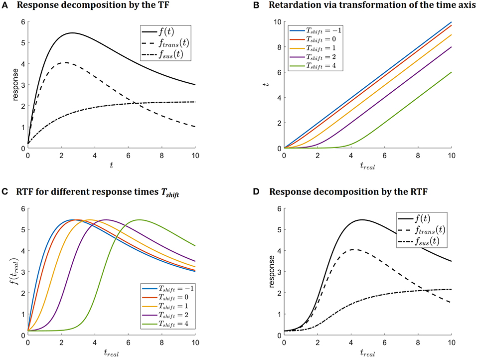
Figure 1. (A) Illustrates decomposition of the response function (4) into sustained f_sus and transient f_trans parts. (B) Illustrates the transformation of the time axis which is introduced to retard the response curve. The impact on the response function is depicted in (C). Decomposition of the retarded response function f(t_real) = f_sus(t_real) + f_trans(t_real) is shown in (D) for T_shift = 2.

2.3. The Retarded Transient Dynamics

Depending on the application setting, the transient dynamics of the modeled compounds do not immediately set in at t = 0 but with some delay. I therefore suggest to account for this by applying a non-linear transformation

$\begin{array}{ll}t(t_{\text{real}})={log}_{10}(10^{t_{\text{real}}}+10^{T_{\text{shift}}})-{log}_{10}(1+10^{T_{\text{shift}}})& (6)\end{array}$

of the real measurement time-axis t_real with a single parameter T_shift. This transformation is of the following qualitative form:

$\begin{array}{ll}t(t_{\text{real}})={log}_b(b^{t_{\text{real}}}+b^{T_{\text{shift}}})-{log}_b(1+b^{T_{\text{shift}}})& (7)\end{array}$

$\begin{array}{ll}={log}_b(b^{t_{\text{real}}}+c_1)+{log}_b(c_2)& (8)\end{array}$

$\begin{array}{ll}={log}_b(c_2{t}_{\text{real}}+c_1{c}_2)& (9)\end{array}$

where b denotes the basis of the logarithm. In addition, the two constants $c_1:=b^{T_{\mathrm{\text{shift}}}}$ and $c_2:={(1+b^{T_{\mathrm{\text{shift}}}})}^{-1}$ are introduced.

Rewriting the transformation (6) as (7)-(9) shows that the suggested transformation basically corresponds to a linear transformation of the time axis at the log-scale. As logarithm base, b = 10 in (6) is chosen. The transformation (6) is illustrated in Figure 1B and shows that the time shift T_shift in the suggested parametrization determines the location of the kink. This position of the kink is the time point for the real time axis t_real, where the response time becomes linear, i.e., where the immediate response (4) kicks in. Thus, it can be interpreted as the response time.

The curvature of the kink in the transformation (6) is depend on t_real and therefore, the transformation is not invariant with respect to unit transformation

$\begin{array}{ll}{t}_{\text{real}}\mapsto \text{const.}\times t_{\text{real}}& (10)\end{array}$

of the time axis. Thus, (6) is modified by rescaling with the observed time interval t_range = max(t_real) − min(t_real) to the time interval [0,10], as depicted in Figure 1B. The transformation of the time axis, then finally reads

$\begin{array}{ll}t(t_{\text{real}})={log}_{10}(10^{t_{\text{real}}\times 10/t_{\text{range}}}+10^{T_{\text{shift}}})-{log}_{10}(1+10^{T_{\text{shift}}}).& (11)\end{array}$

Plugging the non-linear time transformation (11) into the immediate response function (4) yields the retarded transient function

$\begin{array}{l}{f}_{\text{RTF}}\left(t_{\text{real}},{\theta }_{\text{RTF}}\right)=A_{\text{sus}}\left(1-e^{-\frac{t\left(t_{\text{real}},T_{\text{shift}}\right)}{{\tau }_1}}\right)\\ +A_{\text{trans}}\left(1-e^{-\frac{t\left(t_{\text{real}},T_{\text{shift}}\right)}{{\tau }_1^{\prime }}}\right)e^{-\frac{t\left(t_{\text{real}},T_{\text{shift}}\right)}{{\tau }_2}}+p_0& (12)\end{array}$

with ${\theta }_{\mathrm{\text{RTF}}}:=\left\{A_{\mathrm{\text{sus}}},A_{\mathrm{\text{trans}}},{\tau }_1,{\tau }_1^{\prime },{\tau }_2,p_0,T_{\mathrm{\text{shift}}}\right\}$ which will be applied in the following to approximate solutions of ODEs which in the systems biology setting often have transient temporal shapes.

Figure 1C illustrates how the shape of f(t_real, θ_RTF) depends on the response time parameter T_shift: the larger the response time parameter T_shift, the later the response. The colors coincide with Figure 1B. Finally, Figure 1D illustrates the transient and sustained parts of the response for T_shift = 2.

2.4. Fitting to ODE Solutions

In systems biology, ODE modeling is currently the state-of-the-art approach for the mathematical modeling of regulatory networks. The RTF approach (11), (12) can complement the ODE approach in two ways: first, by applying the RTF approach to already existing ODE models in order to provide an approximating mathematical representation which is easy to handle computationally, for instance for integration into a multi-scale model. Second, the RTF can be used instead of an ODE-based model. For both purposes, it is important to assess the abilities of the RTF for approximating ODE solutions.

The abilities of the RTF (11), (12) for approximating the dynamics of ODE models are evaluated by fitting the function to a component x_j of the ODE solutions. For this task, least-squares estimation

$\begin{array}{ll}\widehat{\theta }(x_j)=arg{\displaystyle \underset{{\theta }_{\text{RTF}}}{min}}{\displaystyle \sum _i}{(f_{\text{RTF}}(t_i,{\theta }_{\text{RTF}})-x_j(t_i))}^2& (13)\end{array}$

was performed. Moreover, the root-mean-square error

$\begin{array}{ll}\text{RMSE}\left(x_j\right)=\sqrt{\frac{1}{n}{\displaystyle \sum _i^n}{\left(x_j\left(t_i\right)-f_{\text{RTF}}\left(t_i,\widehat{\theta }\right)\right)}^2}& (14)\end{array}$

is calculated. Finally, the scaled RMSE

$\begin{array}{ll}\text{Approx. err:}=\frac{\text{RMSE}}{{\displaystyle {max}_i}(x_j(t_i))-min(x_j(t_i))}& (15)\end{array}$

is interpreted as an approximation error.

2.5. Fitting to Data

For experimental data, the parameters of the transient function f_i ≡ f_RFT(t_i, θ_RTF) or of an ODE-based model f_i ≡ O_i(x(t_i, u_i, θ_D), θ_O) are estimated by maximum likelihood estimation. For data

$\begin{array}{ll}{y}_i=f_i+{\epsilon }_i,{\epsilon }_i~N(0,{\sigma }_i^2)& (16)\end{array}$

with independently distributed Gaussian errors with variances ${\sigma }_i^2$, the likelihood is given by

$\begin{array}{l}L(\theta )=\rho (y|\theta )={\displaystyle \prod _i\rho }(y_i|\theta )\\ ={\displaystyle \prod _i\frac{1}{\sqrt{2\pi }{\sigma }_i}}\exp \left(-\frac{{(y_i-f(t_i,\theta ))}^2}{2{\sigma }_i^2}\right).& (17)\end{array}$

Then, the negative log-likelihood is

$\begin{array}{ll}-2log\left(L\left(\theta \right)\right)=-2{\displaystyle \sum _i}log\left(\frac{1}{\sqrt{2\pi }{\sigma }_i}\right)+{\displaystyle \sum _i}{\left(\frac{y_i-f\left(t_i,\theta \right)}{{\sigma }_i}\right)}^2.& (18)\end{array}$

As a result, maximum likelihood estimation

$\begin{array}{ll}\widehat{\theta }=arg{\displaystyle \underset{\theta }{max}}L(\theta )& (19)\end{array}$

coincides with least-squares

$\begin{array}{ll}\widehat{\theta }=arg{\displaystyle \underset{\theta }{min}}{\chi }^2(\theta )& (20)\end{array}$

where the least-squares objective function

$\begin{array}{ll}{\chi }^2\left(\theta \right):={\displaystyle \sum _i}{\left(\frac{y_i-f\left(t_i,\theta \right)}{{\sigma }_i}\right)}^2=-2logL\left(y|\theta \right)+\text{const.}& (21)\end{array}$

is minimized for parameter estimation.

2.6. Reducing Overfitting

If a small number of data points is available, it is essential to prevent overfitting. Overfitting is excessive adaptation of the model and its parameters to measurement errors [20]. In the following, three strategies for diminishing the overfitting problem are suggested.

2.6.1. Parameter Constraints

To prevent overfitting which is recommended if a limited amount of data is available, the same time constant ${\tau }_1\equiv {\tau }_1^{\prime }$ for induction of the transient response and for the sustained response can be assumed. We used the resulting five-parameter transient function TF in Lucarelli et al. [21] previously for analyzing the transcription of TGFβ target genes. In that application, the analyses were performed for pairs of time-courses for treated and untreated cells and the resulting time dependencies were used for clustering of genes.

Moreover, it is possible to specify bounds for the parameters as a restriction to reasonable ranges. These bounds should be independent of physical units, i.e., they should be invariant under scaling of the data or sampling times. Technically, bounds are also required for making reasonable initial guesses for the numerical optimization of equation (21). Moreover, setting parameter bounds strongly improves the convergence behavior in the course of numerical non-linear least squares optimization [22].

Assuming that the sampling times t_real1, …, t_realN of the data points used for fitting were reasonably chosen, the minimal sampling interval $\underset{i}{min}(t_{\mathrm{\text{real}}i+1}-t_{\mathrm{\text{real}}i})$ can be utilized to define a lower bound for the time scales. In addition, the amplitudes can be restricted based on the range (max(y)−min(y)) of the data points y = {y₁, …, y_N}. Likewise, the data offset can be constrained by the minimal and maximal data point.

Table 1 summarizes my suggestions for the setting of parameter bounds. These recommendations were derived by manual inspection of the fitted function for experimental data.

TABLE 1

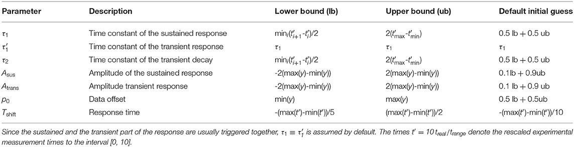
Table 1. Suggested default values and parameter bounds.

If overfitting is a minor issue, these bounds can be relaxed, e.g., if existing ODE models are approximated and these bounds turn out to be too stringent.

2.6.2. Model Reduction

The second strategy for diminishing overfitting is reduction of the number of fitted parameters in an automatic data-driven manner. This means that the complexity of the model is reduced because the available data can be sufficiently described with a simplified model. Such a data-driven simplification of the model equations has been termed model reduction [23].

For model reduction of the RTF and, in turn, decreasing overfitting issues, the likelihood ratio test is utilized. The likelihood ratio test is a well-established statistical test for assessing whether additional parameters yield a significant improvement [24]. The likelihood ratio test is interpreted in a reverse manner as it is commonly done in backward elimination procedures [25]. As test statistic, the log-likelihood ratio of two models is evaluated which in my notation corresponds to

$\begin{array}{ll}\text{LLR}={\chi }_{(1)}^2(\widehat{\theta })-{\chi }_{(2)}^2(\widehat{\theta })& (22)\end{array}$

where ${\chi }_{(1)}^2$ denotes the least-squares objective function of the reduced model and ${\chi }_{(2)}^2$ denotes the objective function of the full model.

Here, the following backward elimination procedure is suggested:

1. Testing whether there is time retardation, i.e., if T_shift parameter is significantly different from the lower bound. If not significant, T_shift is set to the lower bound which is T_shift = −2 by default.

2. Testing whether the model is in agreement with a constant. If not significant, we set T_shift = τ₁ = τ₂ = A_sus = A_trans = 0.

3. Testing whether the offset p₀ is significantly different from zero. If not significant, we set p₀ = 0.

Application-specific prior knowledge can be utilized on top of this. As an example, if the data is pre-processed and the minimal value is subtracted, the offset parameter p₀ might be omitted in advance. If the responses are, furthermore, known to be strictly positive, the lower bounds of the amplitudes A_trans and A_sus can then be set to zero.

2.6.3. Enhancing and Attenuating Responses

The RTF according to (12) allows amplitudes A_sus and A_trans with positive or negative signs. In many application settings, however, it might be a reasonable assumption, that the sustained and transient part of the response have the same direction, i.e., are both either enhancing, or both attenuating. This presumption also reduces the amount of overfitting and often yields much more realistic outcomes. It can be achieved by restricting both amplitudes to positive numbers and introducing a sign-constant. If such a model is fitted, two optimization runs are required for both signs and the better fit is selected.

2.7. Implementation

The RTF approach can be implemented in any modeling or curve fitting software based on equations (11) and (12). An implementation of the presented RTF approach is provided within the Data2Dynamics (D2D) modeling environment [26] which is freely available. In order to guide custom implementations, some important technical aspects of my implementation are discussed in the following.

Since the transient function is non-linear, −2logL(θ) is not convex and local optima can occur. Therefore, multi-start optimization [27] is suggested and has been performed to find the global optimum, i.e., the best possible fit. For fitting the six parameters of the RTF, ten random initial guesses were drawn which turned out as sufficient for finding the global optimum based on visual inspection of the outcomes.

In order to fit responses with positive and negative signs, two subsequent fits are required. Moreover, model reduction as described in section 2.6.2 might be desired. For multi-start optimization, both tasks have to be performed for each initial guess. In D2D, this functionality has been implemented in arFitTransient.m. If D2D's standard multi-start optimization function is intended to be utilized, the standard function in Advanced/arFits.m has to be replaced by TransientFunction_library/arFits.m by modifying Matlab's search path properly.

Further implementation details and examples for applying the RTF approach are provided at the website of the D2D github repository https://github.com/Data2Dynamics/d2d/wiki/RTF.

3. Results

In this chapter, in section 3.1 it is first demonstrated that the retarded transient function (RTF) can accurately describe the dynamics of ODE models as they commonly occur in systems biology. Specifically, two aspects will be addressed. First the abilities for accurate approximations are investigated and proven which is a prerequisite for applying the RTF as mathematical modeling approach directly to data. Second, it will be demonstrated that established ODE models can be approximated if required, e.g., as components of a multi-scale model, which might require explicit functions for technical reasons.

In section 3.2, the RTF approach is then evaluated and compared with ODE models for predicting the dynamics from measurements. For this purpose, simulated data is generated and the accuracy of the estimated time courses is assessed by the comparison to the known dynamics (“ground truth”).

3.1. Approximation of ODE Models

The dynamics of biochemical interactions can be translated into ODE models in order to describe the time-dependency of the concentrations of molecular compounds. In this publication, the accuracy of the RTF approach for modeling of such time courses is assessed based on a subset of nine benchmark models [2] that do not comprise discontinuities, i.e., so-called events [28]. The ODEs published in the original papers are application specific special cases of (1).

1. The Bachmann model [29] describes the JAK2/STAT5 signaling pathway in murine blood forming cells. The model comprises 25 biochemical species representing EPO receptors states, STAT5 activation and translocation to the nucleus, as well as activation of SOCS and CIS proteins that act as negative feedback regulators. In total, these compounds were evaluated in 23 experimental conditions. In addition, the ODE model has 29 dynamic parameters.

2. The Becker model [30] describes the binding of EPO to EPO receptors as well as receptor turnover and degradation in a murine proB cell line and has ten dynamic parameters. The model comprises ODEs for different configurations of EPO and EPO receptors. The ODE model describes a binding assay with six EPO doses and the dynamics of eight compounds for one default EPO dose.

3. The Boehm model [31] has been published for the evaluation of homo- and hetero-dimerization of the transcription factor isoforms STAT5A and STAT5B. The model has seven dynamic parameters and describes nine compounds for one ligand concentration.

4. The Bruno model [32] has been used for investigation of the activity of Arabidopsis carotenoid cleavage dioxygenase 4. It describes carotenoid biosynthesis and the formation of carotenoid-derived signaling molecules. The model comprises 13 dynamic parameters and contains seven dynamic compounds which are evaluated for six different experimental conditions.

5. The Crauste model [33] describes CD8 T cell differentiation after a viral infection. The model describes several differentiation stages (naive, early effector, late effector and memory cells). The model contains twelve dynamic parameters for the description of five dynamic compounds in one experimental condition.

6. The Fiedler model [34] describes Raf/MEK/ERK signaling in synchronized HeLa cells upon stimulation with two MEK and ERK inhibitors (Sorafenib and U0126). The model has 15 dynamic parameters for the dynamics of six biochemical species evaluated in three different experimental conditions.

7. The Raia model [35] describes the interleukin-13 induced activation of JAK/STAT signaling in B-cells and lymphoma cell lines. The pathway consists of interleukin receptors, JAK2 and STAT5 as signaling mediators as well as of two feedback regulators (SOCS3 and CD274) that are described at the mRNA and protein levels. The model comprises 18 dynamic parameters and incorporates 16 biochemical compounds in four different experimental conditions.

8. The Schwen model [36] is a dynamic model for insulin binding to receptors in mouse hepatocytes. This ODE model has 13 dynamic parameters and describes eleven dynamic variables in seven experimental conditions.

9. Finally, the Swameye model [37] has been published to demonstrate shuttling of STAT5 from the nucleus back to the cytoplasm. This model has ten dynamic parameters and contains twelve dynamic variables in a single experimental condition. It describes the activation and dimerization of STAT5 upon EPO treatment as well as the translocation of dimers between cytosol and nucleus.

The retarded transient function (RTF) was fitted to the dynamics of the ODE solutions of all these models resulting in 797 fits in total. In addition to a single fit using the initial guess specified in Table 1, multi-start optimization with ten random initial guesses was performed for approximation errors larger than 5%. Figure 2 shows representative examples in panel (A) as well as worst case scenarios (B) and the overall distribution of the approximation error.

FIGURE 2

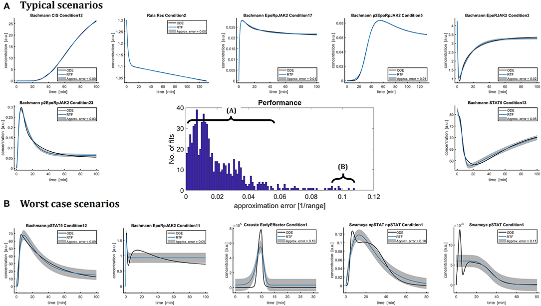
Figure 2. The dynamics of 797 numerical ODE solutions x(t) from the nine different benchmark models were fitted by the RTF in order to assess and illustrate the capacity of the RTF (11), (12) for approximating ODE solutions (black lines). The underlying equations of the ODE models originate from the original publications and were taken from the benchmark collection [2]. The fitting has been performed based on (13), (18)–(21). The histogram in the center shows the distribution of the resulting approximation errors (15). These errors are also plotted as gray bands and their magnitudes are indicated in the figure legends. In more than half of all fits, the difference between both approaches is hardly visible. For the other cases, the RTF most of the time describes the dynamics qualitatively. (A) Shows typical scenarios for approximating ODE solutions by the RTF. Limitations of the approach are pointed out in (B). Here, five representative fits with large approximation errors are plotted.

In 83.8% of all evaluated cases, the approximation error, i.e., the normalized RMSE (15) between RTF and x(t) is smaller than 5%. In 58.3% of cases the approximation error is even smaller than 2% and the difference between the RTF approximation and the ODE solution is hardly visible.

In order to assess the quality of the RTF approximation, it should be kept in mind, that accuracy and reproducibility of experimental data is a major limitation and characteristic of cell biology. This is due to the fact that living cells with individual and unique histories and attributes are investigated. Depending on the cell system, the experimental conditions and the measurement technique, relative errors of 10–20% are common [38]. Moreover, in many applications a minimum concentration change by a factor of 1.5 is requested as a minimum effect size with biological relevance. In light of these aspects, the RTF approach exhibits a convincing performance for describing the major shape characteristics.

All 797 fits are available as Supplementary File 1 to demonstrate the abilities of the RTF approach for the approximation of the typical dynamics of cellular signaling models. Since a few cases where optimization of the RTF parameter did not converged to the global optimum are suspected, the agreement could even be improved by increasing the number of random initial guesses. Moreover, the bounds specified in Table 1 could be relaxed in order to further improve the agreement between ODEs and RTF. However, since this analysis is used as a foundation for the analysis of experimental data, the same bounds as in the next section were chosen at this point.

In some few cases, the RTF approach has limited performance, e.g., for time courses with multiple response peaks. Panel (B) shows five worst case scenarios resulting in approximation errors between 9% and 11%. For the second plot, “Bachmann EpoRpJAK2 Conditon1,” the ODE solution has two distinct response peaks, but the fitted RTF can only describes the first peak. The ODE model shown in the third plot of panel (B), “Crauste EarlyEffector Condition1,” is initially zero and then shows a rather quick and strong peak around t = 10 min. This peak is again only roughly approximated by the RTF with an overall approximation error of around 10%.

The forth and fifth plots in panel (B), “Swameye npSTAT Condition1” and “Swameye pSTAT Condition1,” exhibit a second delayed response which cannot be captured by the RTF. For pSTAT activation “Swameye pSTAT5 Condition1,” the RTF approach fails to describe an initial fast and short activation. This result could be improved by using additional prior knowledge, i.e., by utilizing the fact that prior to stimulation, pSTAT is known to be zero and only positive response amplitudes A_sus and A_trans are biologically reasonable. All trajectories of the Swameye model contain a second, more or less pronounced response which originates from the shuttling of STAT5 through the nucleus and cannot be closely approximated by the RTF approach. In the original publication [37], this shuttling process has been described by a delay differential equation (DDE), i.e., a model which is not within the primary scope of this paper. Later, the delay was approximated in Schelker et al. [18] by an ODE model utilizing the so-called linear chain trick [39]. This model version was published in Hass et al. [2] as a benchmark model and therefore analyzed in this manuscript. Taking these circumstances into account, it is not surprising that the RTF exhibits limited capabilities. On the other hand, this model nicely exposes some limitations of the RTF approach.

3.2. Fitting of Data

In the previous section, it has been demonstrated that in most cases the presented RTF approach can accurately approximate the dynamics of pathway models based on ODEs. In the current section, the capabilities for the fitting of data is evaluated. Compared to traditional data-based ODE modeling, this approach is a complementary and convenient modeling strategy especially for cases where either too little data is available for building a comprehensive network model, or in situations where only a single or a few outputs are of interest.

In systems biology, the availability of experimental data is usually strongly limited because analysis of living cells is elaborate and expensive. Time course data, as an example, rarely comprise more than ten time points. However, the dynamics is usually evaluated for several “conditions,” e.g., for multiple stimulation strengths and/or different genetic backgrounds. These experimental conditions correspond to distinct initial conditions or parameters in the ODE model.

The Bachmann model, as an example, contains 23 experimental conditions. These conditions represent different combinations of 14 doses of ligand treatment, with/without Actinomycin co-treatment of wild type cells or cells where CIS or SOCS3 is over-expressed. In order to evaluate the abilities of the RTF approach on a wide variety of possible dynamic shapes, all combinations of these conditions were evaluated, i.e., all 14 EPO doses for all eight wild-type/over-expression settings.

For each of the resulting 112 conditions, a single time course data set was simulated with 10 equidistant different time points between 0 and 100 min for one out of all 25 dynamic variables x. In total, this results in 2,800 simulated data sets which are individually fitted using the ODE model and the RTF. As measurement error, a typical relative error of 10% was assumed. If 10% was below 1e-5, the standard deviation was set to 1e-5.

For fitting the ODE model, the true parameter values that were used for simulation were also taken as initial guess. Moreover, a local multi-start optimization with ten different starting points around the true parameters was applied. For this purpose, each parameter vector was randomly perturbed by adding uniform numbers from the range [−1, 1] at the log₁₀-scale.

Figure 3 shows typical outcomes for the ODE model and the RTF approach in panel (A). RMSEs (14) between the fitted time course and the time course for the true underlying ODE model were calculated for both approaches for the fine time grid with 300 time points which was also used for plotting the solid lines. In order to obtain comparable numbers for all fits, the RMSEs were divided by the mean measurement error

$\begin{array}{ll}\bar{\sigma }=\frac{1}{10}{\displaystyle \sum _{i=1}^{10}}{\sigma }_i& (23)\end{array}$

over ten simulated data points.

FIGURE 3

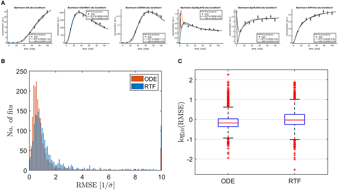
Figure 3. (A) Shows six typical outcomes for fitted RTF models (blue lines) (11), (12) and ODE models (brown lines) in order to compare the outcomes of both modeling approaches for fitting of data. Fitting has been performed based on (13), (18)–(21). The black lines represent the solutions of the ODE equation models which are taken from Hass et al. [2] for published parameter values and presumed as true dynamics for the simulation of the data. In most cases, both approaches provide estimated curves which are close to the true dynamics and the performances coincide. Moreover, there are some examples, where either one or both approaches provide biased outcomes. (B) Shows the resulting RMSEs (14) as histograms. All values above 10 are plotted in the rightmost bin. On average, the ODE approach results in smaller RMSEs but the RTF is only slightly inferior. This qualitative outcome is confirmed by the boxplot shown in (C). It shows that the differences between the individual fits are much larger than the average performance loss of the RTF.

Histograms and boxplots of the scaled RMSEs are displayed in panel (B) and (C). The ODE model, which has been used to generate the data, shows a slightly superior performance, i.e., smaller RMSEs. The median of the scaled RMSE is 0.465 for the ODE model and 0.608 for the RTF. If constant time courses with RMSEs close to zero are omitted, the median is 0.662 for the ODE model and 0.926 for the RTF approach. In both cases, the median performance benefit of the ODE model is by a factor of 20–40 smaller than the differences between individual data sets/time courses because the standard deviation of the RMSEs over all fits is 5.26 for the ODE model and 5.44 for the RTF.

For the same analysis, Figure 4 shows the scaled RMSE as a scatterplot. The RMSEs of both approaches are correlated. All points above the diagonal have larger RMSEs for the RTF approach. For all points below the diagonal, the RTF approach outperforms the ODE model. Figures 4A–J illustrate extreme cases, i.e., scenarios where both approaches have small or large RMSEs, or fits where one approach strongly outperforms the other. This illustration, again, confirms that the average difference in performance is much smaller than the difference between individual fits.

FIGURE 4

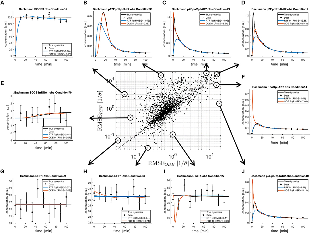
Figure 4. Comparison of both, the fitted RTFs (11), (12) and the fitted ODEs from Bachmann et al. [29] to simulated data with published parameter values. Again, fitting has been performed based on (13), (18)–(21). The scatterplot in the middle shows RMSEs (14) between fitted and true dynamics (black lines) for both modeling approaches. For all points above the diagonal, the ODE model outperforms the RTF. However, there are also several examples where the RTF result in smaller RMSEs. Ten fits for extreme scenarios are plotted in (A–J).

Supplementary File 2 provides the results for all 2,800 fits of the RTF without the true dynamics and without the fitted DE model. This file can be inspected in order to obtain an unbiased impression about the fitted dynamics of the RTF approach. According to the subjective appraisal of the author, the results are very close to solutions which would be guessed by an experienced user. In Supplementary File 3, the same fits are plotted together with the true and fitted ODE solutions which illustrates the underlying dynamics as well as the results of both modeling approaches.

Nevertheless, on average the ODE model proves to be advantageous due to the knowledge and utilization of the model structure which has been used to generate the data. This benefit, however, is a factor of 20–40 smaller than the difference between individual fits and might therefore be acceptable in practice. Moreover, in real application settings the advantage of the ODE model is even smaller because in this case the underlying regulatory network is unknown and is also an imperfect approximation of the real biological process. Based on these findings, the RTF approach seems to be a very promising complementary mathematical modeling strategy for settings where comprehensive data, which is required for establishing a comprehensive pathway model, is not or not yet available.

4. Discussion and Summary

Mechanistic ordinary differential equation (ODE) models are the state-of-the-art approach for modeling cellular processes because models can be defined by translating interactions between cellular compounds. The Biomodels database [40, 41], for instance, currently contains 762 ODE models, i.e., more than 83% of the models which are assigned to a modeling approach are classified as an ODE model. Since for such models each model component has its counterpart in the real biological process, this approach provides strong abilities for interpretations and also for predictions of the system's behavior.

In the presented study, the ODE model has been assumed as the truth, e.g., data has been generated based on published ordinary differential equation models. Hence, ODE modeling has been considered as gold-standard and the fitted outcomes of the ODE models have to outperform alternative modeling approaches since all available knowledge, i.e., model structure and data is entirely exploited.

One drawback of ODE-based models is the need for rather large and comprehensive amounts of experimental data for calibration of the unknown model parameters. This is true even if only a few, specific components are of interest, for example the input-output behavior of a signaling pathway. Moreover, elaborate model discrimination procedures are required in order to find a proper model structure. In addition, the models typically increase in size because all relevant states, compounds and interactions have to be considered. Model reduction [23, 42, 43] is a non-trivial task and since usually all dynamic states are coupled, reduced representations describe the dynamic behavior only in an approximate manner.

Some alternative modeling approaches have been suggested as a replacement for ODE models, e.g., if the system is too large, if only a specific input-output behavior is of interest, or if the amount of available data is too small. However, all these approaches have serious limitations. Logical models, as an example, describe the input-output behaviors only in a discrete manner. Constraint-based models neither provide unique predictions nor statistical confidence intervals. Traditional functional estimation methods, like smoothing splines or polynomials are not tailored to the shape of typical temporal responses. Such approaches require densely sampled time-courses in order to provide realistic curves. Moreover, tuning parameters that control the amount of smoothing are difficult to choose. Therefore, these approaches are not yet available as applicable tools for the modeling of the dynamics of cellular compounds.

In contrast, the retarded transient function (RTF) approach suggested in this publication is tailored to typical dynamic response curves observed in cellular signaling pathways. Some basic differences between the RTF approach and ODE-based models are summarized in Table 2. The parameters of the RTF can be nicely interpreted as response time and amplitudes and time constants of a transient and a sustained response fraction. Based on nine benchmark models, it was possible to show that the suggested function can accurately describe the dynamics of solutions of ODE models. Moreover, for fitting simulated data, it could be shown that in terms of root-mean-squared-errors the fitted RTF is almost as good as the true underlying ODE model.

TABLE 2

Table 2. Comparison of major characteristics of RTF- and ODE-based modeling.

As summarized in Figure 5, the presented implementation allows for fast and simple evaluations of the systems dynamics. First, the RTF is fitted to either an existing ODE model or to experimental data. In a second step, the fitted functions are translated to executable Matlab functions. Those functions, then, can be conveniently called for evaluating the time dependency of the concentration of a dynamic compound. This facility is very valuable for integrating mathematical models of cellular processes into multi-scale models, i.e., computational models describing the behavior at the tissue-, organ- or even whole body level based on the processes at the level of individual cells which is currently a major methodological challenge in systems biology [44, 45].

FIGURE 5

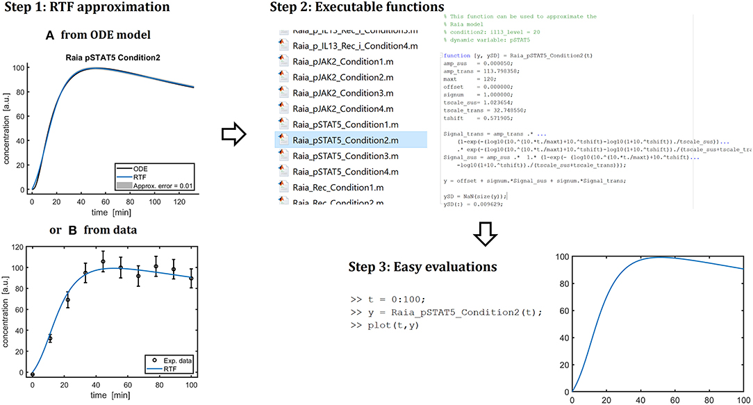
Figure 5. Summary of the presented approach. As a first step, the retarded transient function (RTF) can be applied to approximate ODE solutions (A) or can be fitted to data directly (B). My implementation can generate Matlab code with the fitted parameters (“Step 2”). Then, these function can be called conveniently to evaluate the dynamics of a specific compound in a specific experimental condition (“Step 3”). Moreover, the explicit form of a fitted RTF enables an easy transfer to other applications and modeling frameworks.

Of course, the presented approach also has its limitations. On the one hand, the RTF approach does not provide mechanistic insights. On the other hand, the scope of dynamic shapes is restricted. By construction, the RTF cannot describe several peaks or oscillations and the RTF approach should, therefore, only be applied if such features do not occur or do not play a prominent role. If the RTF is applied for the approximation of existing ODE models, the performance can be evaluated and tested, e.g., in terms of the RMSE. The RTF might then turn out to be inappropriate for ODE models which exhibit an oscillating behavior, delays, or discontinuous dynamics subsequent to multiple perturbations. If the RTF approach is applied for the fitting of data, the measurements should neither be too sparse nor should they be sampled at improper time scales in order to reduce the risk of biased estimation or that important dynamic features are not captured by the model.

The problem of biased estimation and the risk for wrong predictions, however, is a general issue of all modeling approaches, especially in the case of small amounts of experimental data. In my analysis, the median performance loss was 20–40 times smaller than the standard deviation between different fits. The presented RTF approach tends to produce smooth outcomes because only a single maximum/minimum can be captured. This seems to be a reasonable solution for the general trade-off between bias and variance, since the predicted dynamics tend to be plain instead of hypothesizing intricate temporal behavior.

Some tasks remain and are intended to be tackled in the future. First, a theoretical justification for the amazing abilities of the suggested RTF approach is desirable. For this purpose, the class of ODE systems which are exactly solved by the RTF or where the RTF occurs as approximate solution, e.g., for calculations of perturbations, has to be derived and linked to classical rate laws.

Another task consists of linking multiple experimental conditions which originate from different initial conditions, e.g., doses of a ligand. In the current formulation, each initial condition is treated independently and fitted RTFs has distinct and unrelated parameters. Instead, one could describe the dose dependency of individual parameters of the RTF by other explicit functions, e.g., by hill equations which are frequently applied for describing dose dependencies in systems biology [46]. This would then allow for predictions of the time and dose dependency using explicit functions. As a final task, the potential of the RTF approach for multi-scale modeling has to be investigated in order to evaluate its applicability and suitability.

5. Conclusion

A major goal of systems biology is the establishment of mathematical models that describe the behavior of living cells at the level of molecular compounds. Here, the retarded transient function (RTF) has been introduced as a curve fitting approach which is tailored to dynamic modeling of cellular compounds. It has successfully been shown that the approach both provides accurate estimates of the underlying dynamics and facilitates valuable interpretations and, thus, serve as a valuable complement of the traditional ODE-based modeling.

Data Availability Statement

The analyzed benchmark models are available at https://github.com/Benchmarking-Initiative/Benchmark-Models including the analyzed data. The analyses were performed using the Data2Dynamics (D2D) modeling environment which is available at https://github.com/Data2Dynamics/d2d. In D2D, the RTF approach is available including toy model examples in the download folder Examples/ToyModels/TransientFunction. Basic functions including the analyses made for the paper are described in the online wiki of the D2D framework https://github.com/Data2Dynamics/d2d/wiki/RTF.

Author Contributions

CK designed the approach, performed the analyses, and wrote the manuscript.

Funding

This work was supported by the German Ministry of Education and Research by grant EA:Sys (FKZ031L0080) and by the German Research Foundation (DFG) under Germany's Excellence Strategy (CIBSS-EXC-2189-2100249960-390939984). The article processing charge was funded by the German Research Foundation (DFG) and the University of Freiburg in the funding program Open Access Publishing.

Conflict of Interest

The author declares that the research was conducted in the absence of any commercial or financial relationships that could be construed as a potential conflict of interest.

Acknowledgments

I would like to thank Lukas Refisch, Janine Egert, and especially Eva Brombacher for proofreading and language editing.

Supplementary Material

The Supplementary Material for this article can be found online at: https://www.frontiersin.org/articles/10.3389/fphy.2020.00070/full#supplementary-material

Supplementary File 1. RTF approach (blue lines) for all 797 ODE solutions (black lines) from the nine benchmark models. The approximation error is denoted in the legends and plotted as gray band.

Supplementary File 2. RTF approach for the 2,800 simulated data sets. The plots are provided in order to give readers an unbiased impression about the results of the RTF approach.

Supplementary File 3. RTF approach together with the fitted ODE model and the true ODE solution for all 2,800 simulated data sets. These plots indicate differences between the RTF and the ODE modeling approaches.

The plots of the three supplementary files are also available in higher resolution at https://github.com/clemenskreutz/RTF.

References

1. Wolkenhauer O. Systems Biology - Dynamic Pathway Modelling. (2006). Available online at: http://citeseerx.ist.psu.edu/viewdoc/summary?doi=10.1.1.2.7592

Google Scholar

2. Hass H, Loos C, Raimúndez-Álvarez E, Timmer J, Hasenauer J, Kreutz C. Benchmark problems for dynamic modeling of intracellular processes. Bioinformatics. (2019) 35:3073–82. doi: 10.1101/404590

PubMed Abstract | CrossRef Full Text | Google Scholar

3. Simonoff JS. Smoothing Methods in Statistics. New York, NY: Springer Science & Business Media (2012).

Google Scholar

4. Wahba G. Smoothing noisy data with spline functions. Numerische Mathematik. (1975) 24:383–93. doi: 10.1007/BF01437407

CrossRef Full Text | Google Scholar

5. Cressie N. The origins of kriging. Math Geol. (1990) 22:239–52.

Google Scholar

6. Watson GS. Smooth regression analysis. Sankhyā Ind J Stat Ser A. (1964) 26:359–72.

Google Scholar

7. Cleveland WS. Robust locally weighted regression and smoothing scatterplots. J Am Stat Assoc. (1979) 74:829–36. doi: 10.1080/01621459.1979.10481038

CrossRef Full Text | Google Scholar

8. Bradley RA, Srivastava SS. Correlation in polynomial regression. Am Stat. (1979) 33:11–4. doi: 10.1080/00031305.1979.10482644

CrossRef Full Text | Google Scholar

9. Seber GAF, Wild CJ. Nonlinear Regression. New York, NY: Wiley (1989).

Google Scholar

10. Royston P, Sauerbrei W. Multivariable Model-Building: A Pragmatic Approach to Regression Anaylsis Based on Fractional Polynomials for Modelling Continuous Variables. Vol. 777. Chichester: John Wiley & Sons (2008).

Google Scholar

11. Heinonen M, Yildiz C, Mannerström H, Intosalmi J, Lähdesmäki H. Learning unknown ODE models with Gaussian processes. arXiv:180304303 (2018).

Google Scholar

12. Gao P, Honkela A, Rattray M, Lawrence ND. Gaussian process modelling of latent chemical species: applications to inferring transcription factor activities. Bioinformatics. (2008) 24:i70–5. doi: 10.1093/bioinformatics/btn278

PubMed Abstract | CrossRef Full Text | Google Scholar

13. Albert R, Othmer HG. The topology of the regulatory interactions predicts the expression pattern of the segment polarity genes in Drosophila melanogaster. J Theor Biol. (2003) 223:1–18. doi: 10.1016/S0022-5193(03)00035-3

PubMed Abstract | CrossRef Full Text | Google Scholar

14. Klamt S, Saez-Rodriguez J, Lindquist JA, Simeoni L, Gilles ED. A methodology for the structural and functional analysis of signaling and regulatory networks. BMC Bioinformatics. (2006) 7:56. doi: 10.1186/1471-2105-7-56

PubMed Abstract | CrossRef Full Text | Google Scholar

15. Wittmann DM, Krumsiek J, Saez-Rodriguez J, Lauffenburger DA, Klamt S, Theis FJ. Transforming Boolean models to continuous models: methodology and application to T-cell receptor signaling. BMC Syst Biol. (2009) 3:98. doi: 10.1186/1752-0509-3-98

PubMed Abstract | CrossRef Full Text | Google Scholar

16. Liu B, Hagiescu A, Palaniappan SK, Chattopadhyay B, Cui Z, Wong WF, et al. Approximate probabilistic analysis of biopathway dynamics. Bioinformatics. (2012) 28:1508–16. doi: 10.1093/bioinformatics/bts166

PubMed Abstract | CrossRef Full Text | Google Scholar

17. Aldridge BB, Saez-Rodriguez J, Muhlich JL, Sorger PK, Lauffenburger DA. Fuzzy logic analysis of kinase pathway crosstalk in TNF/EGF/insulin-induced signaling. PLoS Comput Biol. (2009) 5:e1000340. doi: 10.1371/journal.pcbi.1000340

PubMed Abstract | CrossRef Full Text | Google Scholar

18. Schelker M, Raue A, Timmer J, Kreutz C. Comprehensive estimation of input signals and dynamics in biochemical reaction networks. Bioinformatics. (2012) 28:i529–34. doi: 10.1093/bioinformatics/bts393

PubMed Abstract | CrossRef Full Text | Google Scholar

19. Hindmarsh AC, Brown PN, Grant KE, Lee SL, Serban R, Shumaker DE, et al. SUNDIALS: suite of nonlinear and differential/algebraic equation solvers. ACM Trans Math Softw. (2005) 31:363–96. doi: 10.1145/1089014.1089020

CrossRef Full Text | Google Scholar

20. Chicco D. Ten quick tips for machine learning in computational biology. BioData Min. (2017) 10:35. doi: 10.1186/s13040-017-0155-3

PubMed Abstract | CrossRef Full Text | Google Scholar

21. Lucarelli P, Schilling M, Kreutz C, Vlasov A, Boehm ME, Iwamoto N, et al. Resolving the combinatorial complexity of smad protein complex formation and its link to gene expression. Cell Syst. (2018) 6:75–89. doi: 10.1016/j.cels.2017.11.010

PubMed Abstract | CrossRef Full Text | Google Scholar

22. Schweiger T. The performance of constrained optimization for ordinary differential equation models. (Bachelor thesis). University of Freiburg, Freiburg, Germany (2017).

23. Maiwald T, Hass H, Steiert B, Vanlier J, Engesser R, Raue A, et al. Driving the model to its limit: profile likelihood based model reduction. PLoS ONE. (2016) 11:e0162366. doi: 10.1371/journal.pone.0162366

PubMed Abstract | CrossRef Full Text | Google Scholar

24. Cox DR, Hinkley DV. Theoretical Statistics. Boca Raton, FL: Chapman and Hall/CRC (1979).

Google Scholar

25. Hocking RR. A Biometrics invited paper. The analysis and selection of variables in linear regression. Biometrics. (1976) 32:1–49. doi: 10.2307/2529336

CrossRef Full Text | Google Scholar

26. Raue A, Steiert B, Schelker M, Kreutz C, Maiwald T, Hass H, et al. Data2Dynamics: a modeling environment tailored to parameter estimation in dynamical systems. Bioinformatics. (2015) 31:3558–60. doi: 10.1093/bioinformatics/btv405

PubMed Abstract | CrossRef Full Text | Google Scholar

27. Raue A, Schilling M, Bachmann J, Matteson A, Schelke M, Kaschek D, et al. Lessons learned from quantitative dynamical modeling in systems biology. PLoS ONE. (2013) 8:e74335. doi: 10.1371/journal.pone.0074335

PubMed Abstract | CrossRef Full Text | Google Scholar

28. Fröhlich F, Theis FJ, Rädler JO, Hasenauer J. Parameter estimation for dynamical systems with discrete events and logical operations. Bioinformatics. (2016) 33:1049–56. doi: 10.1093/bioinformatics/btw764

PubMed Abstract | CrossRef Full Text | Google Scholar

29. Bachmann J, Raue A, Schilling M, Böhm ME, Kreutz C, Kaschek D, et al. Division of labor by dual feedback regulators controls JAK2/STAT5 signaling over broad ligand range. Mol Syst Biol. (2011) 7:516. doi: 10.1038/msb.2011.50

PubMed Abstract | CrossRef Full Text | Google Scholar

30. Becker V, Schilling M, Bachmann J, Baumann U, Raue A, Maiwald T, et al. Covering a broad dynamic range: information processing at the erythropoietin receptor. Science. (2010) 328:1404–8. doi: 10.1126/science.1184913

PubMed Abstract | CrossRef Full Text | Google Scholar

31. Boehm ME, Adlung L, Schilling M, Roth S, Klingmüller U, Lehmann WD. Identification of isoform-specific dynamics in phosphorylation-dependent STAT5 dimerization by quantitative mass spectrometry and mathematical modeling. J Proteome Res. (2014) 13:5685–94. doi: 10.1021/pr5006923

PubMed Abstract | CrossRef Full Text | Google Scholar

32. Bruno M, Koschmieder J, Wuest F, Schaub P, Fehling-Kaschek M, Timmer J, et al. Enzymatic study on AtCCD4 and AtCCD7 and their potential in forming acyclic regulatory metabolites. J Exp Biol. (2016) 67:5993–6005. doi: 10.1093/jxb/erw356

CrossRef Full Text | Google Scholar

33. Crauste F, Mafille J, Boucinha L, Djebali S, Gandrillon O, Marvel J, et al. Identification of nascent memory CD8 T cells and modeling of their ontogeny. Cell Syst. (2017) 4:306–17. doi: 10.1016/j.cels.2017.01.014

PubMed Abstract | CrossRef Full Text | Google Scholar

34. Fiedler A, Raeth S, Theis FJ, Hausser A, Hasenauer J. Tailored parameter optimization methods for ordinary differential equation models with steady-state constraints. BMC Syst Biol. (2016) 10:80. doi: 10.1186/s12918-016-0319-7

PubMed Abstract | CrossRef Full Text | Google Scholar

35. Raia V, Schilling M, Böhm M, Hahn B, Kowarsch A, Raue A, et al. Dynamic mathematical modeling of IL13-induced signaling in Hodgkin and primary mediastinal B-cell lymphoma allows prediction of therapeutic targets. Cancer Res. (2011) 71:693–704. doi: 10.1158/0008-5472.CAN-10-2987

PubMed Abstract | CrossRef Full Text | Google Scholar

36. Schwen LO, Schenk A, Kreutz C, Timmer J, Rodriguez MMB, Kuepfer L, et al. Representative sinusoids for hepatic four-scale pharmacokinetics simulations. PLoS ONE. (2015) 10:e0133653. doi: 10.1371/journal.pone.0133653

PubMed Abstract | CrossRef Full Text | Google Scholar

37. Swameye I, Müller T, Timmer J, Sandra O, Klingmüller U. Identification of nucleocytoplasmic cycling as a remote sensor in cellular signaling by data-based modeling. Proc Natl Acad Sci USA. (2003) 100:1028–33. doi: 10.1073/pnas.0237333100

CrossRef Full Text | Google Scholar

38. Kreutz C, Bartolome Rodriguez MM, Maiwald T, Seidl M, Blum HE, Mohr L, et al. An error model for protein quantification. Bioinformatics. (2007) 23:2747–53. doi: 10.1093/bioinformatics/btm397

PubMed Abstract | CrossRef Full Text | Google Scholar

39. Smith HL. An Introduction to Delay Differential Equations With Applications to the Life Sciences. Vol. 57. New York, NY: Springer (2011).

Google Scholar

40. Li C, Donizelli M, Rodriguez N, Dharuri H, Endler L, Chelliah V, et al. BioModels database: an enhanced, curated and annotated resource for published quantitative kinetic models. BMC Syst Biol. (2010) 4:92. doi: 10.1186/1752-0509-4-92

PubMed Abstract | CrossRef Full Text | Google Scholar

41. Chelliah V, Juty N, Ajmera I, Ali R, Dumousseau M, Glont M, et al. BioModels: ten-year anniversary. Nucl Acids Res. (2015) 43:542–8. doi: 10.1093/nar/gku1181

PubMed Abstract | CrossRef Full Text | Google Scholar

42. Apri M, de Gee M, Molenaar J. Complexity reduction preserving dynamical behavior of biochemical networks. J Theor Biol. (2012) 304:16–26. doi: 10.1016/j.jtbi.2012.03.019

PubMed Abstract | CrossRef Full Text | Google Scholar

43. Radulescu O, Gorban AN, Zinovyev A, Noel V. Reduction of dynamical biochemical reactions networks in computational biology. Front Genet. (2012) 3:131. doi: 10.3389/fgene.2012.00131

PubMed Abstract | CrossRef Full Text | Google Scholar

44. Heiner M, Gilbert D. Biomodel engineering for multiscale systems biology. Prog Biophys Mol Biol. (2013) 111:119–28. doi: 10.1016/j.pbiomolbio.2012.10.001

PubMed Abstract | CrossRef Full Text | Google Scholar

45. Vicini P. Multiscale modeling in drug discovery and development: future opportunities and present challenges. Clin Pharmacol Therapeut. (2010) 88:126–9. doi: 10.1038/clpt.2010.87

PubMed Abstract | CrossRef Full Text | Google Scholar

46. Goutelle S, Maurin M, Rougier F, Barbaut X, Bourguignon L, Ducher M, et al. The Hill equation: a review of its capabilities in pharmacological modelling. Fundament Clin Pharmacol. (2008) 22:633–48. doi: 10.1111/j.1472-8206.2008.00633.x

PubMed Abstract | CrossRef Full Text | Google Scholar