
94% of researchers rate our articles as excellent or good
Learn more about the work of our research integrity team to safeguard the quality of each article we publish.
Find out more
ORIGINAL RESEARCH article
Front. Phys. , 17 January 2020
Sec. Statistical and Computational Physics
Volume 7 - 2019 | https://doi.org/10.3389/fphy.2019.00220
This article is part of the Research Topic New Numerical and Analytical Methods for Nonlinear Partial Differential Equations with Applications in Quantum Physics View all 18 articles
 Nauman Ahmed1,2
 Mehreen Fatima3
 Dumitru Baleanu4,5
 Kottakkaran Sooppy Nisar6
 Ilyas Khan2*
 Muhammad Rafiq7
 Muhammad Aziz ur Rehman1
 Muhammad Ozair Ahmad8
In this paper, two structure-preserving nonstandard finite difference (NSFD) operator splitting schemes are designed for the solution of reaction diffusion epidemic models. The proposed schemes preserve all the essential properties possessed by the continuous systems. These schemes are applied on a diffusive SEIQV epidemic model with a saturated incidence rate to validate the results. Furthermore, the stability of the continuous system is proved, and the bifurcation value is evaluated. A comparison is also made with the existing operator splitting numerical scheme. Simulations are also performed for numerical experiments.
Mathematical modeling has a prominent role in describing physical phenomena in various disciplines of mathematics, physical sciences, social sciences, engineering, life sciences, and many more [1–6]. The transmission of infectious diseases and the control of their spread can be studied effectively by constructing mathematical models for various strategies like vaccination and quarantine. The word quarantine denotes forced isolation or being cut off from interactions with others. Quarantine is an effective intervention process for restraining the spread of infection by isolating individuals who are affected by the disease. Such isolation has been adopted to decrease the communication of infectious diseases like dengue, measles, smallpox, cholera, leprosy, tuberculosis, and many more.
Epidemic models, that is, mathematical models of infectious diseases, are a simplified way to illustrate the transmission dynamics of the complicated nonlinear processes and complex behavior of an infectious disease in individuals within a population. These are deterministic models that are used to allocate the population to different subclasses or compartments, describing a particular stage of the epidemic. The incidence rate, which is proportional to the number of susceptible and infected persons, is an important parameter of compartment-based epidemic models. The mathematical models of infectious diseases are often based on bilinear incidence rate βSI, but a more concise approach to use the saturated incidence rate rather than the bilinear incidence rate. In the saturated incidence rate , if number of infected individuals I becomes very large, approaches the saturation level. The infection force is measured by βI, which describes the penetration of the disease into a fully susceptible population. is used to measure the inhibition effect of behavioral change of susceptible persons. Liu and Yang [7] proposed the SEIQV epidemic model, which uses the saturated incidence rate. The model is expressed as:
The variables and parameters of the model are defined as:
S(t) = Susceptible persons at time t,
E(t) = Exposed persons at time t,
I(t) = Infected persons at time t,
Q(t) = Quarantined persons at time t,
V(t) = Vaccinated persons at time t,
b = Rate of recruitment,
β = Rate of transmission,
μ = Rate of natural death,
ϵ = Rate of death due to disease in infected compartment,
α = Parameter that measures psychological or inhibitory effects,
γ = Rate at which infected individuals are being vaccinated infected persons,
σ = Rate at which exposed persons become infected,
ω = Rate at which infected individuals are being vaccinated susceptible persons,
ϕ = Rate at which infected individuals are being vaccinated quarantined persons,
q1, q2, q3 = Effective quarantine probabilities.
The above model (1)–(5) assumes a homogeneous population, where the population mixes in such a way that there is no difference between person in one place and person in another place. However, in actual scenarios, the disease may spread faster in one place than in another because of different circumstances like different weather conditions, etc. Hence, it is essential for the variables to depend on space also. Therefore, we extend system (1)–(5) to make it a reaction-diffusion system by adding a diffusion term.
with the initial conditions:
The boundary conditions are no flux,
Epidemic models always demonstrate two equilibrium points: the disease-free equilibrium (DFE) point and the endemic equilibrium (EE) point. The DFE point exists if R0 < 1, where R0 is the reproductive number, which basically measures the occurrence of disease. The EE point exists if R0 > 1. This implies that the SEIQV reaction-diffusion system (6–10) always converges to the DFE point or EE point if R0 < 1 or R0 > 1, respectively. Analytical solution of the SEIQV epidemic system is not possible, so we have to use numerical techniques to find its solution. Note that the numerical technique must show the same behavior as is possessed by the continuous SEIQV reaction-diffusion epidemic system.
In this work, we propose two operator-splitting NSFD methods, one explicit and one implicit. These methods are used to solve the SEIQV epidemic model with diffusion. As S, E, I, Q, and V are population sizes and evaluated in absolute scale, we propose NSFD methods because they give a positive solution. Also, the convergence of the proposed NSFD operator splitting methods toward the equilibrium points is the same as the convergence of continuous an SEIQV reaction-diffusion epidemic system. The proposed splitting methods are designed with the aid of rules given by Mickens [8]. In the recent era, positivity preserving FD methods have gained importance, as many physical dynamical systems possess the positivity property [9–11]. The NSFD method presented by Mickens [8, 12, 13] has becomes an effective and important structure-preserving FD method for solving differential equations. In epidemic models, population dynamics and population size cannot be negative, so the numerical technique must be a positivity-preserving technique. Various authors have used different positivity-preserving numerical techniques for the approximate solution of epidemic models: see, for example [14–22].
In this work, we also show the numerical stability of the SEIQV epidemic model with diffusion and evaluate the bifurcation value of the vaccination parameter ω with the aid of the Routh-Hurwitz method.
The model (6–10) has two equilibrium points [7], the DFE point and EE point. The DFE point is:
and the EE point is:
where,
Reproductive number R0 is given as:
R0 is the reproductive value. Now, if R0 < 1, the model acquires a DFE point, and if R0 > 1, the model acquires an EE point.
We evaluated the small perturbation S1(x, t), E1(x, t), I1(x, t), Q1(x, t), and V1(x, t) so that (6)–(10) is linearized at the EE point (S*, E*, I*, Q*, V*), as discussed in Chakrabrty et al. [23].
Suppose a Fourier series solution is demonstrated for Equations (23)–(27) of the form:
Here, k = nπ/2, (n = 1, 2, 3,…) exhibits the value of the wave number for the node n. Substituting Equations (28)–(32) in the system (23)–(27), the system is converted into:
The variational matrix for the system (33)–(37) is:
where,
The characteristics equation for matrix is:
The expressions for ξ1, ξ2, ξ3, ξ4, and ξ5 with diffusion and without diffusion are mentioned in Islam and Haider [24].
The Routh-Hurwitz stability criterion gives:
and
The Table 2 reflects the numerical stability of the equilibrium point against the various cases, as discussed in Table 1.
Considering the vaccination parameter ω, to find its bifurcation value, a11, a12, are used instead of S*, E*, I*, Q*, and V*.
The Routh-Hurwitz criterion for stability gives:
where the values of ξ1, ξ2, ξ3, ξ4, and ξ5 are obtained from the expression of the characteristic equation (without diffusion) given in paper [24].
f5(ω) = 0 gives the value of bifurcation for ω. This value transfers the stability of a continuous model from stable to unstable. f5(ω) = 0 provides the bifurcation value ω = 0.228360507. The EE point is stable for ω less than ω = 0.228360507.
For the bifurcation value of vaccination parameter ω, the values of S*, E*, I*, Q*, and V* are replaced into a11, a12, to
The Routh-Hurwitz criterion for stability gives:
f5(ω) = 0 gives ω = 0.24144152. The EE point is stable therefore for any value less than ω = 0.24144152.
It can be seen that the value of bifurcation of ω for the system with diffusion is greater than value of bifurcation of ω for the system without diffusion.
In this section, we apply two proposed and classical splitting methods to the SEIQV reaction-diffusion epidemic model with diffusion. Operator-splitting techniques very effectively handle the nonlinearity and complexity of reaction-diffusion equations. Therefore, these techniques are used frequently by several researchers for the solution of nonlinear differential equations [23, 25–33]. The SEIQV epidemic model with diffusion is split in two ways. The nonlinear reaction equations are split in the first step as,
and the diffusion equations are split in the second step as:
Now, we apply forward and backward Euler methods with operator splitting on the system (6)–(7).
where and at mτ, m = 0, 1, … and 0 + ih, i = 0, 1, … reflects difference approximations of S, E, I, Q, and V. The values of , , , , and are the values at the half time step. Both forward and backward Euler methods have same process at first step, but, at the second half step of time, they have different procedures. Since the forward Euler operator splitting method is explicit, we use:
For the backward Euler method, we use:
For the proposed NSFD operator splitting methods, we implement the rules constructed by Mickens [8]. The technique for both explicit and implicit schemes is similar at the first half time step:
A positive solution desires that if:
The techniques for the implicit and explicit NSFD schemes are not similar for the second half of the time step. The procedure for the explicit NSFD scheme is as follows:
We use an implicit procedure for the second NSFD method at the second half of the time step:
where,
In finite difference operator splitting techniques, the step involving the reaction term is unconditionally stable because it is solved exactly [25, 26]. On the other hand, the step involving the diffusion term has different stability in different techniques. The explicit procedure has conditional stability in the region:
while the implicit procedure has unconditionally stability [25, 26]. The accuracy of both schemes is O(τ) and O(h2) for all the methods under study.
Equations (64)–(65) in the reaction step of both proposed methods preserve the property of positivity depicted by the continuous SEIQV model, as there is no negative term involved in (64)–(65).
As far as the diffusion step is concerned, the proposed explicit scheme (70)–(74) demonstrates the positivity of the solution if:
so,
which is the condition of stability for the explicit operator-splitting NSFD scheme (70)–(74). This verifies that the explicit NSFD scheme retains the positive solution in the region of stability. M matrix theory has been used for the verification of the positivity of the implicit NSFD method (75)–(79). For more details [34] is referred.
For any positive τ and h, the system described by (75)–(79) is also positive, i.e., Sm > 0, Em > 0, Qm > 0 and Vm > 0, ∀m = 0, 1, 2…
Proof
Equations (75)–(79) can be written as:
In Equations (81)–(85), the letters A, B, C, D, and G represent the square matrices. Where,
The off-diagonal entries of A are a1 = −2λ1, a2 = −λ1, and the diagonal entries are a3 = 1 + 2λ1. The entries of B in the off-diagonal are b1 = −2λ1, b2 = −λ1, and the diagonal entries are b3 = 1 + 2λ2. The entries of C in the off-diagonal are c1 = −2λ3, c2 = −λ3, and the diagonal entries are c3 = 1 + 2λ3. The off-diagonal entries of D are d1 = −2λ4, d2 = −λ4, and the diagonal entries are d3 = 1 + 2λ4. The off-diagonal entries of G are g1 = −2λ5, g2 = −λ5, and the diagonal entries are g3 = 1 + 2λ5. Thus, A, B, C, D, and G are M-matrices, and Equations (81), (82), (83), (84), and (85) are:
If we consider that Sm > 0, Em > 0, Im > 0, Qm > 0, and Vm > 0, then the M-matrix along with (60) implies that the values of all of the state variables, i.e., Sm+1, Em+1, Im+1, Qm+10, and Vm+1 are positive. Hence, the theorem is done by using the principle of mathematical induction.
This theorem is applied for drawing the conclusion that the proposed scheme, which is implicit in nature, guarantees the positive solution unconditionally.
A numerical test is performed on both the points of equilibrium for all the schemes under consideration. The set of parametric values considered for the test problem at disease-free equilibrium point [7] is given as:
b = 0.7, μ = 0.06, σ = 0.7, β = 0.35, γ = 0.15, ω = 0.3, q1 = 0.2, q2 = 0.2, q3 = 0.1, ϕ = 0.4, ϵ = 0.05, α = 2, d1 = 0.05, d2 = 0.01, d3 = 0.001, d4 = 0.01, d5 = 0.01.
For the endemic equilibrium point, the following parametric values are used:
b = 0.7, μ = 0.06, σ = 0.7, β = 0.35, γ = 0.15, ω = 0.06, q1 = 0.2, q2 = 0.2,
q3 = 0.1, ϕ = 0.4, ϵ = 0.05, α = 2, d1 = 0.05, d2 = 0.01, d3 = 0.001, d4 = 0.01, d5 = 0.01.
The initial condition for the model (6)–(10) is:
In this section, graphs of all the state variables against time are presented (for DFE) to illustrate the behavior of the schemes. In Figures 1, 2, we consider h = 0.5, λ1 = 0.3, λ2 = 0.06, λ3 = 0.006, λ4 = 0.06, and λ5 = 0.06.
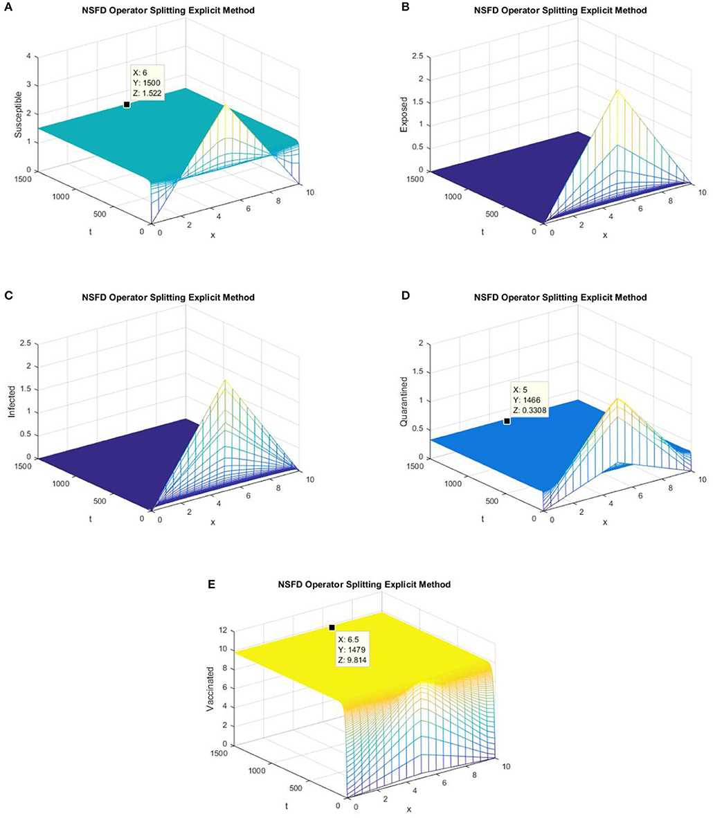
Figure 1. The explicit operator splitting NSFD scheme is used to simulate the graphs (A–E). (A) Mesh graph of S; (B) Mesh graph of E; (C) Mesh graph of I; (D) Mesh graph of Q; (E) Mesh graph of V.
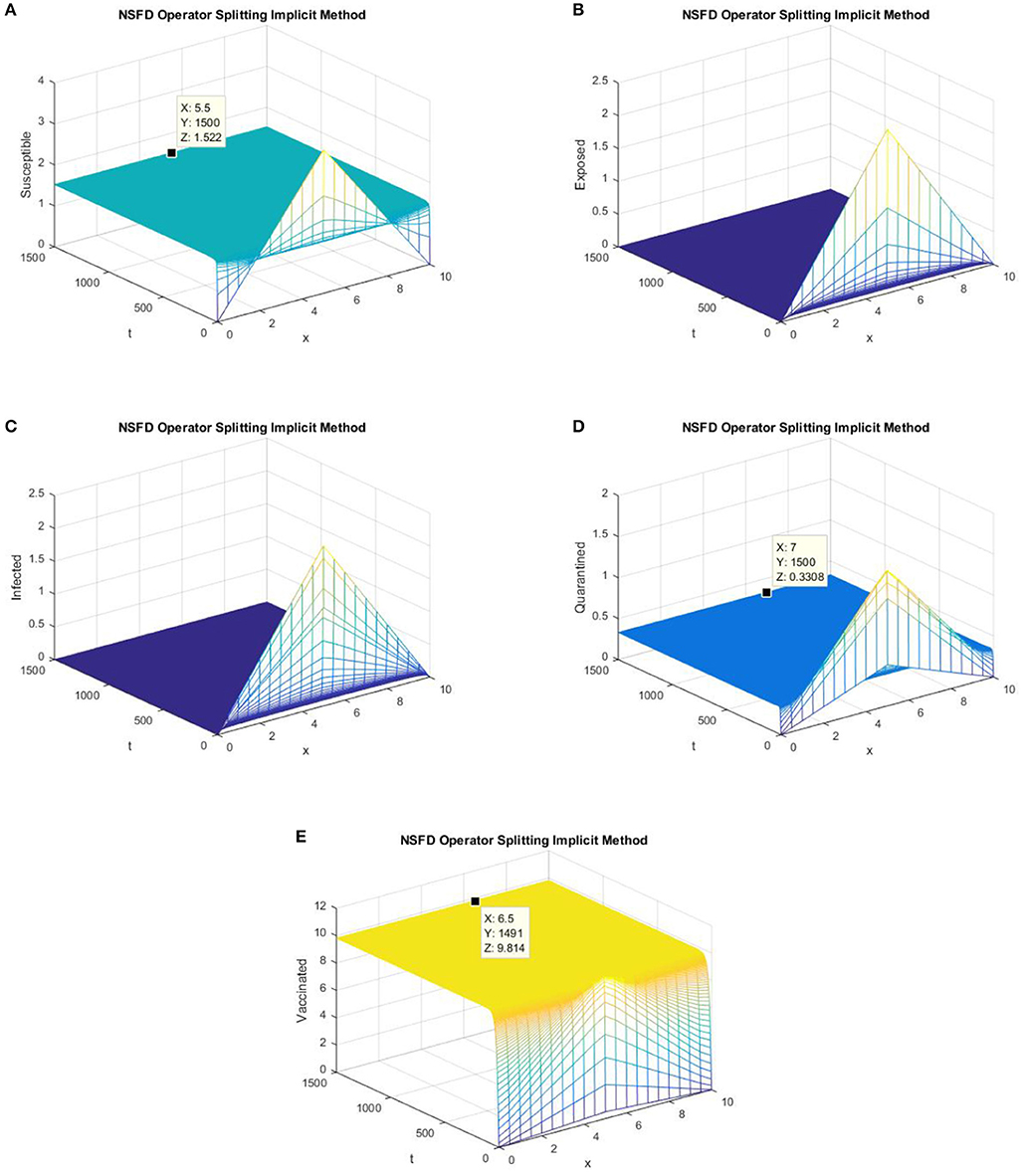
Figure 2. The implicit operator splitting NSFD scheme is used to simulate graphs (A–E). (A) Mesh graph of S; (B) Mesh graph of E; (C) Mesh graph of I; (D) Mesh graph of Q; (E) Mesh graph of V.
Figures 1, 2 validate the preservation of the positivity property in both of the proposed operator splitting NSFD schemes. Also, all the graphs in Figures 1, 2 show that both proposed NSFD schemes achieve convergence to the DFE point. Next, we examine the behavior of forward Euler and backward Euler splitting schemes at different values of h and τ.
In parts (a) and (b) of Figure 3, we take the same values of h and τ as in Figures 1, 2 for the graphs of forward Euler operator splitting scheme and backward Euler operator splitting scheme. The graphs clearly show the failure of the positivity property of both classic schemes. In parts (c) and (d) of Figure 3, both existing splitting schemes converge to the false DFE equilibrium point for susceptible individuals.
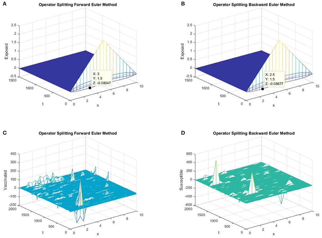
Figure 3. (A) The forward Euler FD operator splitting method is used to simulate the graph of exposed persons for the DFE point at h = 0.5, λ1 = 0.3. (B) The backward Euler FD operator splitting method is used to simulate the graph of susceptible persons for the DFE point at h = 0.5, λ1 = 0.3. (C) The forward Euler FD operator splitting method is used to simulate the graph of susceptible persons for the DFE point at h = 0.5, λ1 = 0.4. (D) The backward Euler FD operator splitting method is used to simulate the graph of susceptible persons for the DFE point at h = 0.5, λ1 = 0.4.
In parts (a) and (b) of Figure 4, we take the same values of h and τ as given in parts (c) and (d) of Figure 3 for the explicit and implicit NSFD operator splitting schemes, respectively. The graphs clearly show that both of the proposed NSFD schemes not only preserve the positivity property but also achieve convergence to the true equilibrium point.
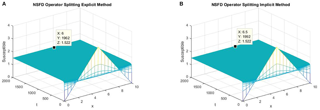
Figure 4. (A) The explicit operator splitting NSFD method is used to simulate the graph of susceptible persons for the DFE point at h = 0.5, λ1 = 0.3. (B) The implicit operator splitting NSFD method is used to simulate the graph of susceptible persons for the DFE point at h = 0.5, λ1 = 0.4.
In this section, we present simulations of the SEIQV epidemic model at the EE point using all of the operator splitting FD schemes. In Figures 5, 6, we consider h = 0.5, λ1 = 0.3, λ2 = 0.06, λ3 = 0.006, λ4 = 0.06, and λ5 = 0.06.
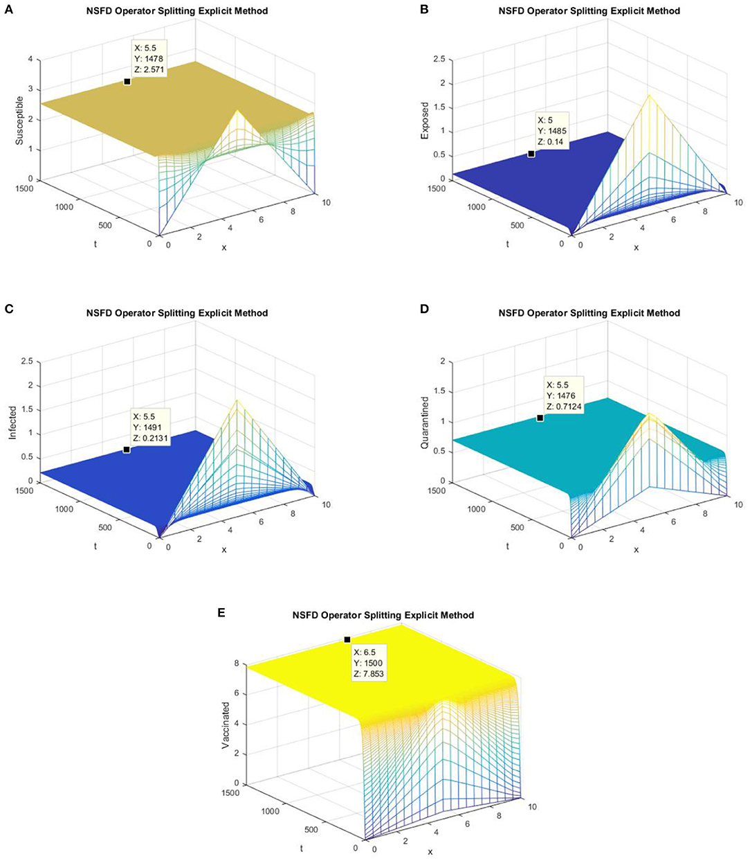
Figure 5. (A) The explicit operator splitting NSFD scheme is used to simulate graphs (A–E). (A) Mesh graph of S; (B) Mesh graph of E; (C) Mesh graph of I; (D) Mesh graph of Q; (E) Mesh graph of V.
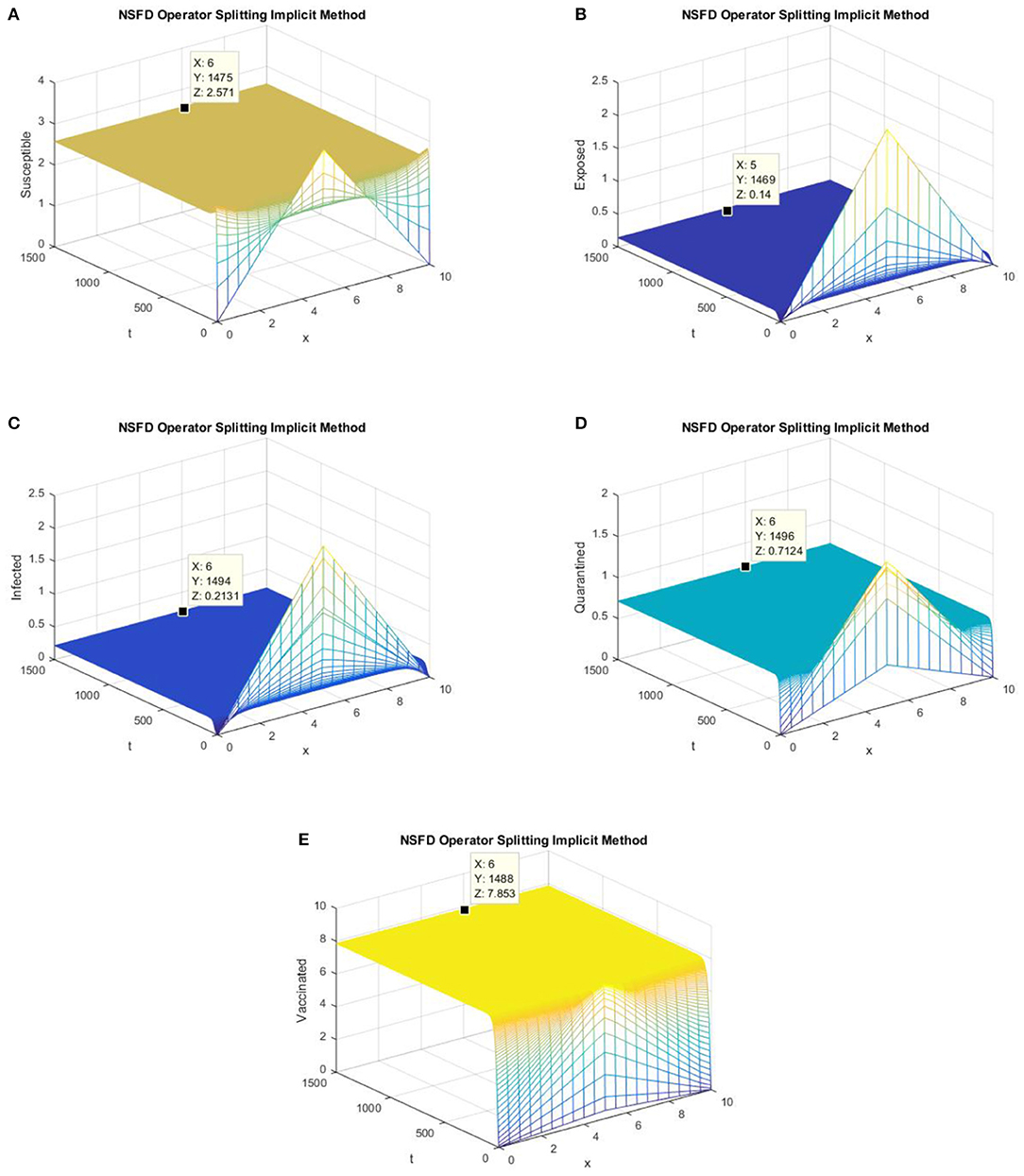
Figure 6. The implicit operator splitting NSFD scheme is used to simulate graphs (A–E). (A) Mesh graph of S; (B) Mesh graph of E; (C) Mesh graph of I; (D) Mesh graph of Q; (E) Mesh graph of V.
Figures 5, 6 depict the graphs of susceptible, exposed, infected, quarantined, and vaccinated individuals for the EE point using the explicit operator splitting NSFD scheme and implicit operator splitting NSFD scheme, respectively. All the graphs in Figures 5, 6 demonstrate that both of the proposed operator splitting NSFD schemes preserve the property of positivity. These graphs also show that both proposed schemes converge to the EE point.
Again, both the forward and backward Euler FD schemes fail to preserve the positivity property and converge to the false EE point, as shown in Figure 7.
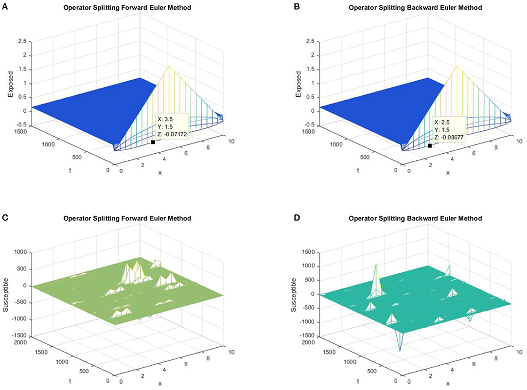
Figure 7. (A) The forward Euler FD operator splitting method is used to simulate the graph of exposed persons for the DFE point at h = 0.5, λ1 = 0.3. (B) The backward Euler FD operator splitting method is used to simulate the graph of exposed persons for the DFE point at h = 0.5, λ1 = 0.3. (C) The forward Euler FD operator splitting method is used to simulate the graph of susceptible persons for the DFE point at h = 0.5, λ1 = 0.4. (D) The backward Euler FD operator splitting method is used to simulate the graph of susceptible persons for the DFE point at h = 0.5, λ1 = 0.4.
Figure 8 shows that the proposed NSFD operator splitting methods are consistent with the continuous reaction-diffusion system as they not only preserve the positivity property but converge to the EE point.
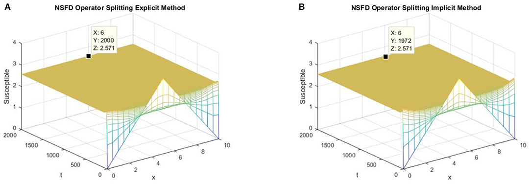
Figure 8. (A) The explicit operator splitting NSFD method is used to simulate the graph of susceptible persons for the DFE point at h = 0.5, λ1 = 0.4. (B) The implicit operator splitting NSFD method is used to simulate the graph of susceptible persons for the DFE point at h = 0.5, λ1 = 0.4.
In this work, we consider the SEIQV reaction-diffusion epidemic model. The stability of the SEIQV model is guaranteed numerically by using criteria defined by Routh-Hurwitz. We also find the bifurcation value of the important vaccination parameter ω of SEIQV epidemic systems with diffusion and without diffusion. We design two novel and efficient operator splitting NSFD schemes for the SEIQV reaction-diffusion system. The NSFD schemes put forth, which are technically operator splitting schemes, possess the same behavior as is possessed by the SEIQV epidemic system. To conclude regarding the designed methods, we present two novel numerical schemes, one of which is explicit and the other of which is implicit in nature. The explicit scheme is more computationally efficient than the implicit scheme, but it has conditional stability while the implicit scheme is stable unconditionally. Both schemes employ structural splitting, due to which they deal adroitly with the nonlinearity of the reaction-diffusion system. These schemes avoid the false chaos that is a part of many existing methods. The positive solution of the SEIQV model is sustained by both schemes. Also, the nature of the stability of equilibria is preserved effectively by the proposed NSFD schemes. It is also shown that classical schemes, in parallel to our proposed schemes, produce chaos, leading to inconsistencies and instabilities numerically. The currently designed schemes are a valuable contribution for finding the solutions of nonlinear dynamical systems comprising differential equations. These NSFD schemes will become very efficient for the solution of one- and multi-dimensional reaction-diffusion population models, auto-catalytic chemical reaction models, and many more.
NA, MR, and MAR designed the study. NA, MF, and MR developed the methodology. NA and MF collected the data. NA, DB, KN, and IK performed the analysis. NA, MF, DB, MA, and IK wrote the manuscript.
The authors declare that the research was conducted in the absence of any commercial or financial relationships that could be construed as a potential conflict of interest.
The authors are grateful to the referees for their suggestions and useful comments on this paper.
1. Ahmed N, Wei Z, Baleanu D, Rafiq M, Rehman MA. Spatio-temporal numerical modeling of reaction-diffusion measles epidemic system. Chaos. (2019) 29:103101. doi: 10.1063/1.5116807
2. Abro KA, Khan I, Nisar KS. Novel technique of Atangana and Baleanu for heat dissipation in transmission line of electrical circuit. Chaos Solitons Fractals. (2019) 129:40–5 doi: 10.1016/j.chaos.2019.08.001
3. Ahmed N, Rafiq M, Baleanu D, Rehman MA. Spatio-temporal numerical modeling of auto-catalytic Brusselator model. Roman J Phys. (2019) 64:110.
4. Gill V, Singh J and Singh Y. Analytical solution of generalized space-time fractional advection-dispersion equation via coupling of sumudu and fourier transforms. Front Phys. (2019) 6:151. doi: 10.3389/fphy.2018.00151
5. Kumar D, Singh J, Al Qurashi M, Baleanu D. A new fractional SIRS-SI malaria disease model with application of vaccines, antimalarial drugs, and spraying. Adv Differ Equ. (2019) 278. doi: 10.1186/s13662-019-2199-9
6. Saqib M, Khan I, Shafie S. Application of fractional differential equations to heat transfer in hybrid nanofluid: modeling and solution via integral transforms. Adv Differ Equ. (2019) 52: doi: 10.1186/s13662-019-1988-5
7. Liu X, Yang L. Stability analysis of an SEIQV epidemic model with saturated incidence rate. Nonlinear Anal Real World Appl. (2012) 13:2671–9. doi: 10.1016/j.nonrwa.2012.03.010
8. Mickens RE. Nonstandard finite difference models of differential equations world scientific (1994).
9. Ahmed N, Rafiq M, Rehman MA, Iqbal MS, Ali M. Numerical modelling of three dimensional Brusselator reaction diffusion system. AIP Adv. (2019) 9:015205. doi: 10.1063/1.5070093
10. Mickens RE. Dynamic consistency: a fundamental principle for constructing nonstandard finite difference schemes for differential equations. J Differ Equ Appl. (2005) 11:645–53. doi: 10.1080/10236190412331334527.
11. Macias-Diaz JE, Puri A. An explicit positivity-preserving finite-difference scheme for the classical Fisher-Kolmogorov-Petrovsky-Piscounov equation. Appl Math Comput. (2012) 218:5829–37. doi: 10.1016/j.amc.2011.11.064
12. Mickens RE. A nonstandard finite difference scheme for a Fisher PDE having nonlinear diffusion. Comput Math Appl. (2003) 45:429–36. doi: 10.1016/S0898-1221(03)80028-7
13. Mickens RE. A nonstandard finite difference scheme for an advection-reaction equation J Diff Eq Appl. (2004) 10:307–1312. doi: 10.1080/10236190410001652838
14. Ahmed N, Rafiq M, Rehman MA, Ali M, Ahmad MO. Numerical modeling of SEIR measles dynamics with diffusion. Commun Math Appl. (2018) 9:315–26.
15. Ahmed N, Shahid N, Iqbal Z, Jawaz M, Rafiq M, Tahira SS, et al. Numerical modeling of SEIQV epidemic model with saturated incidence rate. J Appl Environ Biol Sci. (2018) 8:67–82.
16. Ahmed N, Jawaz M, Rafiq M, Rehman MA, Ali M, Ahmad MO. Numerical treatment of an epidemic model with spatial diffusion. J Appl Environ Biol Sci. (2018) 8:17–29.
17. Chinviriyasit S, Chinviriyasit W. Numerical modeling of SIR epidemic model with diffusion. Appl Math Comp. (2010) 216:395–409. doi: 10.1016/j.amc.2010.01.028
18. Fatima U, Ali M, Ahmed N, Rafiq M. Numerical modeling of susceptible latent breaking-out quarantine computer virus epidemic dynamics. Heliyon. (2018) 4:e00631. doi: 10.1016/j.heliyon.2018.e00631
19. Jansen H, Twizell EH. An unconditionally convergent discretization of the SEIR model. Math Comput Simulat. (2002) 58:147–58. doi: 10.1016/S0378-4754(01)00356-1
20. Rafiq M. Numerical modeling of infectious diseases dynamics. Ph.D. thesis, Lahore, Pakistan: University of Engineering and Technology (2016).
21. Qin W, Wang L, Ding X. A non-standard finite difference method for a hepatitis B virus infection model with spatial diffusion. J Differ Equ Appl. (2014) 20:1641–51. doi: 10.1080/10236198.2014.968565
22. Manna K, Chakrabarty SP. Global stability and a non-standard finite difference scheme for a diffusion driven HBV model with capsids. J Differ Equ Appl. (2015) 21:918–33. doi: 10.1080/10236198.2015.1056524
23. Chakrabrty A, Singh M, Lucy B, Ridland P. Predator-prey model with prey- taxis and diffusion. Math Comput Model. (2007) 46:482–98. doi: 10.1016/j.mcm.2006.10.010
24. Islam S, Haider N. Numerical solution of compartmental model by meshless finite difference methods. Appl Math Comput. (2014) 238:408–35. doi: 10.1016/j.amc.2014.04.014
25. Harwood RC. (2011) Operator splitting method and applications for semilinear parabolic partial differential equations. Ph.D. dissertation. Pullman, WA: Dept. Math., Washington State Univ.
26. Harwood RC, Manoranjan VS, Edwards DB. Lead-acid battery model under discharge with a fast splitting method. IEEE Trans Energy Convers. (2011) 26:1109–17. doi: 10.1109/TEC.2011.2162093
28. Zharnitsky V. Averaging for split-step scheme. Nonlinearity. (2003) 16:1359–66. doi: 10.1088/0951-7715/16/4/310
29. Ansarizadeh F, Singh M, Richards D. Modelling of tumor cells regression in response to chemotherapeutic treatment. Appl Math Model. (2017) 48:96–112. doi: 10.1016/j.apm.2017.03.045
30. Naheed A, Singh M, Lucy D. Numerical study of SARS epidemic model with the inclusion of diffusion in the system. Appl Math Comput. (2014) 229:480–98. doi: 10.1016/j.amc.2013.12.062
31. Naheed A, Singh M, Lucy D. Effect of treatment on transmission dynamics of SARS epidemic. J Infect Non Infect Dis. (2016) 2:16. doi: 10.24966/INID-8654/100016
32. Samsuzzoha MD. A Study on numerical solutions of epidemic models. Ph.D. thesis, Australia: Swinburne University of Technology (2012).
33. Wang H. Q., Numerical studies on the split-step finite difference method for nonlinear Schrödinger equations. Appl Math Comput. (2005) 170:17–35. doi: 10.1016/j.amc.2004.10.066
Keywords: splitting methods, NSFD schemes, positivity, epidemic model, stability, bifurcation value
Citation: Ahmed N, Fatima M, Baleanu D, Nisar KS, Khan I, Rafiq M, Rehman MA and Ahmad MO (2020) Numerical Analysis of the Susceptible Exposed Infected Quarantined and Vaccinated (SEIQV) Reaction-Diffusion Epidemic Model. Front. Phys. 7:220. doi: 10.3389/fphy.2019.00220
Received: 06 October 2019; Accepted: 28 November 2019;
Published: 17 January 2020.
Edited by:
Devendra Kumar, University of Rajasthan, IndiaReviewed by:
Yudhveer Singh, Amity University Jaipur, IndiaCopyright © 2020 Ahmed, Fatima, Baleanu, Nisar, Khan, Rafiq, Rehman and Ahmad. This is an open-access article distributed under the terms of the Creative Commons Attribution License (CC BY). The use, distribution or reproduction in other forums is permitted, provided the original author(s) and the copyright owner(s) are credited and that the original publication in this journal is cited, in accordance with accepted academic practice. No use, distribution or reproduction is permitted which does not comply with these terms.
*Correspondence: Ilyas Khan, aWx5YXNraGFuQHRkdHUuZWR1LnZu
Disclaimer: All claims expressed in this article are solely those of the authors and do not necessarily represent those of their affiliated organizations, or those of the publisher, the editors and the reviewers. Any product that may be evaluated in this article or claim that may be made by its manufacturer is not guaranteed or endorsed by the publisher.
Research integrity at Frontiers

Learn more about the work of our research integrity team to safeguard the quality of each article we publish.