Burst Distribution by Asymptotic Expansion in the Equal Load Sharing Fiber Bundle Model

We derive an asymptotic series expansion for the burst size distribution in the equal load sharing fiber bundle model, a predominant model for breakdown in disordered media. Earlier calculations give expressions with correct asymptotic behavior for large bursts, but low accuracy for small bursts, up to an order of magnitude off. The approximations from the expansion we present here give relative errors of at most several percent when compared with exact results or simulation results for large systems. We also solve the burst size distribution exactly for the Weibull threshold distributions.

1. Introduction

The fiber bundle model [1–4] is a prime example of what Bouchaud calls a metaphorical model [5]; that is, a model which reveals mechanisms that lie hidden beneath layers of complexity in realistic models and are completely lost in phenomenological models. Even in its simplest form, the equal load sharing (ELS) model, the number of papers written on the fiber bundle model may now be counted in the thousands. This is evidence of great richness.

The distribution of bursts, or avalanches, is important in the study of fiber bundle models. Its behavior can signal how close the bundle is to catastrophic failure, even in single samples [6]. There are many variations of the fiber bundle model, but we will only study the ELS model here. We will also limit ourselves to continuous (i.e., infinitesimal) load increase; finite load increases gives a different distribution of bursts [7, 8].

For the ELS model with continuous load increase, Hemmer and Hansen [9] demonstrated that bursts follow a power law with an exponent 5/2 for a wide class of disorder distributions. Sornette [10] derived this power law behavior separately with a different approach. This work was followed up Pradhan et al.[6, 11], who showed that the power law exponent changes to 3/2 as the bundle is approaching catastrophic failure. Raischel et al. [12] showed that this kind of crossover is present also in the γ-model [13], which has a variable range of interaction with the equal and local load sharing model as its two limits.

By following the development of the crossover burst size—that is, the burst size that constitutes the watershed between bursts following the 5/2 law and the bursts following the 3/2 law—it is possible to quantitatively measure of how far the bundle is from collapse. However, this approach has the problem that it requires knowledge of large (and hence rare) bursts, which have poor statistics. It would be better to predict failure from the smallest bursts, which happen often and can be measured with higher accuracy. This makes it important to have access to accurate analytic estimates of these values to compare with. Hence, we provide in this article a method to analytically calculate the burst distribution accurately for small bursts.

2. The Equal Load Sharing Fiber Bundle Model

Consider an equal load sharing fiber bundle model with N fibers [1, 2]. The externally applied force (or load) F is distributed identically on all intact fibers, and a fiber acts as Hookean spring until its elongation reaches a certain threshold, where it breaks. Due to the equal load sharing, fibers will always fail in order from smallest to largest threshold as the load increases.

The thresholds are drawn independently from a probability density p(t), with a corresponding cumulative distribution $P(t)={\int }_{-\infty }^{t}p(u)\mathrm{\text{d}}u$. Let {t_k} be the ordered sequence of thresholds, such that t₁ ≤ t₂ ≤ ··· ≤ t_N. Then the force F_k required to break the kth fiber is

$\begin{array}{ll}{F}_k=\left(N+1-k\right)t_k.& (1)\end{array}$

Equation (1) shows that F_k consists of two factors: the decreasing number of intact fibers N + 1 − k, and the increasing threshold t_k of the kth fiber. Due to the irregularities of {t_k}, F_k doesn't increase or decrease smoothly. Instead, it fluctuates up and down around a general increasing trend. Or decreasing, depending on where in the fracture process we are.

If the force F is the control parameter during the breaking process, this causes bursts (or avalanches) of several fibers that break under the same load. There is a burst of size Δ beginning with the failure of the kth fiber if F_k > F_j for j < k, F_k+j ≤ F_k for j < Δ, and F_k+Δ > F_k. This simply means that when the force reaches F_k, Δ fibers break under that load with no further load increase required, and the burst stops at the Δ + 1th fiber, which is strong enough to withstand the load.

The average of Equation (1) over samples is the load curve [4]

$\begin{array}{ll}\sigma (x)=x\left[1-P(x)\right],& (2)\end{array}$

which is also the limit of equation (1) as N → ∞. Here σ = F/N is the applied force per fiber in the bundle, both broken and intact, and x is the elongation of the fiber bundle. For most threshold distributions σ has a single parabolic maximum at elongation x_c, where 1 − P(x_c) = x_cp(x_c).

The burst distribution is usually defined as D(Δ): the expected number of bursts of size Δ during the breaking of a single fiber bundle [3, 4, 9]. This definition makes D(Δ) ∝ N for large systems, and hence it diverges as N → ∞. We will instead use the notation $\bar{D}(\Delta )=D(\Delta )/N$, with the physical interpretation that $\Delta \bar{D}(\Delta )$ is the fraction of fibers broken in bursts of size Δ — which converges to a finite number as N → ∞.

Hemmer and Hansen [9] showed that for continuous load increase, the burst distribution to first order in N has the asymptotic behavior (as Δ → ∞)

$\begin{array}{ll}\overline{D}(\Delta )\sim C{\Delta }^{-5/2},& (3)\end{array}$

where $C={(2\pi )}^{-1/2}{x}_{c}p{(x_c)}^2{\left[2p(x_c)+x_c{p}^{\prime }(x_c)\right]}^{-1}$. This result is universal for threshold distributions where the load curve has a single parabolic maximum.

Pradhan et al.[6, 11] generalized this asymptotic behavior to threshold distributions starting from a lower limit t₀ ≥ 0, and found that there is a crossover

$\begin{array}{lll}\overline{D}(\Delta )& \sim & C{\Delta }^{-5/2}\left(1-{\text{e}}^{-\Delta /{\Delta }_c}\right)\hfill \\ \hfill & \propto & \{\begin{array}{ll}{\Delta }^{-3/2}\hfill & \text{ for }\Delta \ll {\Delta }_c\hfill \\ {\Delta }^{-5/2}\hfill & \text{ for }\Delta \gg {\Delta }_c,\hfill \end{array}\hfill & (4)\end{array}$

with ${\Delta }_c=4\pi C^{2}p{(x_c)}^{-2}{(t_0-x_c)}^{-2}$ and C as in Equation (3). This crossover to a different exponent as t₀ increases has been proposed as a method to detect imminent failure [3, 6, 11].

Equation (4) is also an asymptotic behavior in the limit Δ → ∞, and hence it also requires information about large bursts (which are rare events) to predict failure. Our goal is to find a way to calculate the burst distribution accurately for small bursts, which the asymptotic expressions in Equations (3, 4) cannot do. To this end, we use a threshold distribution with a lower limit t₀ ≥ 0. The burst distribution is then, to first order in N [4],

$\begin{array}{lll}\overline{D}(\Delta )=\frac{{\Delta }^{\Delta -1}}{\Delta !}& {\displaystyle {\int }_{t_0}^{x_C}{\left[a(t){\text{e}}^{-a(t)}\right]}^{\Delta }a{(t)}^{-1}}\left[1-a(t)\right]p(t)\text{d}t& (5)\end{array}$

for t₀ < x_c, where

$\begin{array}{ll}a(t)=\frac{tp(t)}{1-P(t)}.& (6)\end{array}$

At x_c, the critical elongation of Equation (2), this function satisfies a(x_c) = 1.

3. Exact Burst Distribution

Is it possible to solve the burst distribution exactly? The deciding factor is the function a(t). Instead of first choosing a threshold distribution and then checking whether Equation (5) is solvable, we can instead do it in the opposite order: choose a function a(t) for which the integral can be solved, and then use Equation (6) to find the corresponding threshold distribution.

3.1. Constant a(t)

The simplest expression would be a constant a(t), which implies a(t) = 1 because a(x_c) = 1. This gives $\bar{D}(\Delta )=0$ when inserted into Equation (5). To see why, set a(t) = 1 in Equation (6), which gives the differential equation

$\begin{array}{ll}\frac{p^{\prime }(t)}{p(t)}=-\frac{2}{t},& (7)\end{array}$

with the normalized solution P(t) = 1 − t₀/t for t ∈ [t₀, ∞). This makes the load curve in Equation (2) constant: σ(x) = t₀, i.e., x_c = t₀. Thus, there is no burst distribution and $\bar{D}(\Delta )=0$.

3.2. Power Law a(t)

Other than a(t) = 1, the most intuitive choice for a solvable integral is a power law a(t) = C(k)t^k with k > 0. Inserting this into Equation (6) gives the first-order differential equation

$\begin{array}{ll}p(t)+C(k)t^{k-1}P(t)=C(k)t^{k-1}& (8)\end{array}$

for P(t). It can be solved with the integrating factor method: multiplying the equation with $\mu (t)=\text{exp }\left({\int }_{t_0}^t\mathrm{\text{d}}\tau C(k){\tau }^{k-1}\right)=\text{exp }\left[C(k)\left(t^k-t_0^k\right)/k\right]$ and integrating from t₀ to t gives the solution

$\begin{array}{ll}P(t)=\frac{C(k)}{k}\left[1-{\text{e}}^{\frac{C(k)}{k}\left(t_0^k-t^k\right)}\right].& (9)\end{array}$

Normalization on the interval [t₀, ∞), i.e., P(t = ∞) = 1, yields C(k)/k = 1. Thus,

$\begin{array}{ll}P(t)=1-{\text{e}}^{t_0^k-t^k},& (10)\end{array}$

which is a Weibull distribution with shape parameter k and a lower limit t₀. The lower limit corresponds to breaking all fibers with thresholds t < t₀ from a fiber bundle with P(t) = 1 − e^−tk. Hence the lower limit is equivalent to studying a bundle with P(t) = 1 − e^−tk that has already sustained a damage $d=1-{\mathrm{\text{e}}}^{-t_0^k}$.

The Weibull distribution in Equation (10) has a critical extension $x_c=k^{-1/k}$, which gives a(x_c) = 1, as required for consistency. We can now solve the burst distribution exactly for the Weibull distribution. Inserting a(t) = kt^k and $p(t)=k{t}^{k-1}{\mathrm{\text{e}}}^{t_0^k-t^k}$ into Equation (5) gives

$\begin{array}{lll}\overline{D}(\Delta )=\frac{{\Delta }^{\Delta -1}}{\Delta !}{\displaystyle {\int }_{t_0}^{k^{-1/k}}}& {\left(k{t}^k{\text{e}}^{-k{t}^k}\right)}^{\Delta }{\left(k{t}^k\right)}^{-1}\left(1-k{t}^k\right)k{t}^{k-1}{\text{e}}^{t_0^k-t^k}\text{d}t.\hfill & (11)\end{array}$

Use the substitution z = t^k to get

$\begin{array}{lll}\overline{D}(\Delta )=\frac{{\left(k\Delta \right)}^{\Delta -1}}{\Delta !}{\text{e}}^{t_0^k}& \left[{\displaystyle {\int }_{t_0^k}^{1/k}{z}^{\Delta -1}}{\text{e}}^{-z\left(k\Delta +1\right)}\text{d}z-k{\displaystyle {\int }_{t_0^k}^{1/k}{z}^{\Delta }}{\text{e}}^{-z\left(k\Delta +1\right)}\text{d}z\right].\hfill & (12)\end{array}$

Combining integration by parts and induction yields

$\begin{array}{lll}{\displaystyle {\int }_{t_0^k}^{1/k}\text{d}}z{z}^n{\text{e}}^{-\alpha z}=\frac{n!}{{\alpha }^{n+1}}& [{\text{e}}^{-\alpha t_0^k}{\displaystyle \sum _{i=0}^n\frac{{\left(\alpha t_0^k\right)}^i}{i!}}-{\text{e}}^{-\alpha /k}{\displaystyle \sum _{i=0}^n\frac{{\left(\alpha /k\right)}^i}{i!}}],\hfill & (13)\end{array}$

which gives the exact burst distribution

$\begin{array}{l}\overline{D}(\Delta )=\frac{{\Delta }^{\Delta -1}{\text{e}}^{t_0^k}}{\Delta !(k\Delta +1)}\left[{\text{e}}^{-(\Delta +1/k)}-{\left(k{t}_0^k\right)}^{\Delta }{\text{e}}^{-t_0^k(k\Delta +1)}\right]\\ +\frac{{(k\Delta )}^{\Delta -1}{\text{e}}^{-k\Delta t_0^k}}{\Delta {(k\Delta +1)}^{\Delta +1}}{\displaystyle {\displaystyle \sum }_{i=0}^{\Delta -1}}\frac{{\left[(k\Delta +1)t_0^k\right]}^i}{i!}-\frac{{(k\Delta )}^{\Delta -1}{\text{e}}^{t_0^k-(\Delta +1/k)}}{\Delta {(k\Delta +1)}^{\Delta +1}}{\displaystyle {\displaystyle \sum }_{i=0}^{\Delta -1}}\frac{{(k\Delta +1)}^i}{i!k^i}.& (14)\end{array}$

This expression can easily be evaluated for small bursts, which is what we are interested in. Equation (14) for k = 2 and t₀ = 0 is shown in Figure 1 together with the asymptotic result from Equation (4) and simulation results. The agreement between the exact and simulation results is excellent, particularly for small Δ where finite size effects from the simulations are negligible. The asymptotic result from Equation (4) is inaccurate for small Δ—it is 35% smaller than the exact result for Δ = 1—but becomes more and more accurate as Δ increases, which is consistent with the fact that Equation (4) is asymptotically correct in the limit Δ → ∞.

FIGURE 1

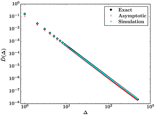
Figure 1. Burst distribution $\bar{D}(\Delta )$ for a Weibull threshold distribution with k = 2 and t₀ = 0. The exact result (black) is Equation (14) and the asymptotic result (red) is Equation (4). The simulation results (turquoise) were found by averaging $\bar{D}(\Delta )$ over 10⁶ sample systems with N = 1024².

For the special case Δ = 1, Equation (14) becomes

$\begin{array}{llll}\overline{D}(\Delta =1)& =\hfill & \frac{{\text{e}}^{t_0^k}}{{(k+1)}^2}\left[k{\text{e}}^{-(1+1/k)}+\left(1-(k+1)k{t}_0^k\right){\text{e}}^{-(k+1)t_0^k}\right].\hfill & (15)\end{array}$

For large bursts Equation (14) is impractical to use, but for Δ ≫ Δ_c the first term is dominant. The equation then simplifies to

$\begin{array}{ll}\overline{D}(\Delta )\simeq \frac{{\Delta }^{\Delta -1}{\text{e}}^{-\Delta }}{\Delta !(k\Delta +1)}{\text{e}}^{t_0^k-1/k}\simeq \frac{{\text{e}}^{t_0^k-1/k}}{\sqrt{2\pi }k}{\Delta }^{-5/2},& (16)\end{array}$

via Stirling's approximation, $\Delta !\simeq \sqrt{2\pi \Delta }{\Delta }^{\Delta }{\mathrm{\text{e}}}^{-\Delta }$. This is the expected asymptotic power law from Equation (3) for the Weibull distribution from Equation (10).

4. Asymptotic Series Expansion

The simplicity of the Weibull threshold distribution is an exception, and for other threshold distributions we cannot expect to find an exact result for the burst distribution. We therefore return to Equation (5) to make an asymptotic series expansion, and note that the equation has the form of a Laplace integral [14]

$\begin{array}{ll}I(\Delta )={\displaystyle {\int }_{t_0}^{x_c}f}(t){\text{e}}^{\Delta \varphi (t)}\text{d}t,& (17)\end{array}$

with

$\begin{array}{ll}f(t)=p(t)\frac{1-a(t)}{a(t)}& (18)\end{array}$

$\begin{array}{ll}\varphi (t)=-a(t)+\text{ln}(a(t)).& (19)\end{array}$

For large Δ the integral is dominated by a small interval around the maximum of ϕ(t) in the interval [t₀, x_c]. In our case ϕ has its maximum at a(t) = 1, i.e., at the critical extension x_c, the upper limit of integration. Hence the asymptotic behavior of Equation (17) as Δ → ∞ is

$\begin{array}{ll}I(\Delta )\sim {\displaystyle {\int }_{x_c-ϵ}^{x_c}f}(t){\text{e}}^{\Delta \varphi (t)}\text{d}t& (20)\end{array}$

where ϵ is a small number. In the small interval [x_c − ϵ, x_c] we can Taylor expand f(t) and ϕ(t) around x_c,

$\begin{array}{l}f(t)=f_1(t-x_c)+f_2{(t-x_c)}^2+f_3{(t-x_c)}^3+···\\ \hfill \varphi (t)={\varphi }_0+{\varphi }_2{(t-x_c)}^2+{\varphi }_3{(t-x_c)}^3+{\varphi }_4{(t-x_c)}^4+···& (21)\end{array}$

Note that f_n and ϕ_n are not identical to the nth derivatives of f(t) and ϕ(t) evaluated at x_c, only proportional to them. The exact expressions for these coefficients in terms of a(t) are shown in Equations (34, 36). Also note that the vanishing terms f₀ = f(x_c) = 0 and ${\varphi }_1\propto {\varphi }^{\prime }(x_c)=0$ (ϕ has its maximum at x_c) are not included here.

In the limit Δ → ∞, when the interval [x_c − ϵ, x_c] can be chosen arbitrarily small, the two first terms in the expansion of ϕ will dominate the others. We therefore separate these terms by factorizing the exponential in the integrand of Equation (20) as

$\begin{array}{ll}\hfill \begin{array}{ccc}\hfill {\text{e}}^{\Delta \varphi (t)}& =\hfill & \text{exp }\left(\Delta {\varphi }_0+\Delta {\varphi }_2{(t-x_c)}^2\right)\hfill \\ \hfill & \times \hfill & \text{exp }\left(\Delta \left[{\varphi }_3{(t-x_c)}^3+{\varphi }_4{(t-x_c)}^4+···\right]\right),\hfill \end{array}& (22)\end{array}$

and then Taylor expand the second factor

$\begin{array}{ll}\hfill \begin{array}{cc}\hfill exp& \left(\Delta \left[{\varphi }_3{(t-x_c)}^3+{\varphi }_4{(t-x_c)}^4+···\right]\right)=1\hfill \\ \hfill & +\Delta \left[{\xi }_{1,3}{(t-x_c)}^3+{\xi }_{1,4}{(t-x_c)}^4+···\right]+{\Delta }^2\left[{\xi }_{2,6}{(t-x_c)}^6+{\xi }_{2,7}{(t-x_c)}^7+···\right]+···,\hfill \end{array}& (23)\end{array}$

which defines ξ_n,m. Inserting these expansions into Equation (20) and extending the lower integration limit back down to t₀ gives

$\begin{array}{ll}\hfill \begin{array}{cc}\hfill I(\Delta )\sim {\text{e}}^{\Delta {\varphi }_0}& {\displaystyle {\int }_{t_0}^{x_c}}{\text{e}}^{\Delta {\varphi }_2{(t-x_c)}^2}\left[f_1(t-x_c)+f_2{(t-x_c)}^2+···\right]\hfill \\ \hfill & \times \{1+\Delta \left[{\xi }_{1,3}{(t-x_c)}^3+···\right]+{\Delta }^2\left[{\xi }_{2,6}{(t-x_c)}^6+···\right]+···\}\text{ d}t.\hfill \end{array}& (24)\end{array}$

The standard approach is to extend the lower limit of integration to −∞ because the integral over [−∞, x_c − ϵ] is subdominant to the integral over [x_c − ϵ, x_c] in the limit Δ → ∞ [14]. But our goal is to use the asymptotic series to calculate an approximation for $\bar{D}(\Delta )$ for small Δ, and we know that the lower limit t₀ is important for small bursts [6].

To solve this integral, multiply the Taylor expansions and separate terms with even and odd powers of t − x_c into I_even(Δ) and I_odd(Δ), respectively. The odd terms are

$\begin{array}{ll}\begin{array}{cc}{I}_{\text{odd}}\hfill & (\Delta )={\text{e}}^{\Delta {\varphi }_0}{\displaystyle {\int }_{t_0}^{x_c}}{\text{e}}^{\Delta {\varphi }_2{(t-x_c)}^2}\{\left[f_1(t-x_c)+f_3{(t-x_c)}^3+···\right]\hfill \\ \hfill & +\Delta \left[{\omega }_{1,5}{(t-x_c)}^5+{\omega }_{1,7}{(t-x_c)}^7+···\right]+{\Delta }^2\left[{\omega }_{2,7}{(t-x_c)}^5+{\omega }_{2,9}{(t-x_c)}^9+···\right]+···\}\text{ d}t,\hfill \end{array}& (25)\end{array}$

where ω_n,m is defined in Equation (38). Then choose $u=\Delta {\varphi }_2{(t-x_c)}^2$, which yields

$\begin{array}{l}{I}_{\text{odd}}(\Delta )=\frac{{\text{e}}^{\Delta {\varphi }_0}}{2\Delta {\varphi }_2}{{{\displaystyle \int }}^{\text{}}}_{\Delta {\varphi }_2{(t_0-x_c)}^2}^0{\text{e}}^u\{\left[f_1+f_3\frac{u}{\Delta {\varphi }_2}+···\right]\hfill \\ +\Delta \left[{\omega }_{1,5}{\left(\frac{u}{\Delta {\varphi }_2}\right)}^2+{\omega }_{1,7}{\left(\frac{u}{\Delta {\varphi }_2}\right)}^3+···\right]+{\Delta }^2\left[{\omega }_{2,7}{\left(\frac{u}{\Delta {\varphi }_2}\right)}^3+{\omega }_{2,9}{\left(\frac{u}{\Delta {\varphi }_2}\right)}^4+···\right]+···\}\text{ d}u,\hfill & (26)\end{array}$

We can now group these terms by the integrands' dependence on Δ:

$\begin{array}{lll}{I}_{\text{odd}}(\Delta )=\frac{{\text{e}}^{\Delta {\varphi }_0}}{2\Delta {\varphi }_2}& ({\Omega }_0(\Delta )+{\Omega }_1(\Delta ){\Delta }^{-1}+{\Omega }_2(\Delta ){\Delta }^{-2}+···),\hfill & (27)\end{array}$

where Ω_n—see Equation (40)—-depends on Δ due to the lower limit of integration.

The even terms in t − x_c are

$\begin{array}{l}{I}_{\text{even}}(\Delta )=e^{\Delta {\varphi }_0}{{{\displaystyle \int }}^{}}_{t_0}^{x_c}{e}^{\Delta {\varphi }_2{(t-x_c)}^2}\{\left[f_2{(t-x_c)}^2+f_4{(t-x_c)}^4+···\right]\\ +\Delta [{\omega }_{1,4}{(t-x_c)}^4+{\omega }_{1,6}{(t-x_c)}^6+···]+{\Delta }^2[{\omega }_{2,8}{(t-x_c)}^8+{\omega }_{2,10}{(t-x_c)}^{10}+···]+···\}dt.& (28)\end{array}$

Since ϕ₂ < 0, choose $u=\sqrt{-\Delta {\varphi }_2}(t-x_c)$. Then

$\begin{array}{ll}\begin{array}{c}{I}_{\text{even}}(\Delta )=\frac{{\text{e}}^{\Delta {\varphi }_0}}{\sqrt{-\Delta {\varphi }_2}}{\displaystyle {\int }_{\sqrt{-\Delta {\varphi }_2}\left(t_0-x_c\right)}^0}{\text{e}}^{-u^2}\{\left[f_2{\left(\frac{u}{\sqrt{-\Delta {\varphi }_2}}\right)}^2+f_4{\left(\frac{u}{\sqrt{-\Delta {\varphi }_2}}\right)}^4+···\right]\hfill \\ +\Delta \left[{\omega }_{1,4}{\left(\frac{u}{\sqrt{-\Delta {\varphi }_2}}\right)}^4+{\omega }_{1,6}{\left(\frac{u}{\sqrt{-\Delta {\varphi }_2}}\right)}^6+···\right]+{\Delta }^2\left[{\omega }_{2,8}{\left(\frac{u}{\sqrt{-\Delta {\varphi }_2}}\right)}^8+{\omega }_{2,10}{\left(\frac{u}{\sqrt{-\Delta {\varphi }_2}}\right)}^{10}+···\right]+···\}\text{d}u.\hfill \end{array}& (29)\end{array}$

Grouping these terms by the integrands' dependence on Δ yields

$\begin{array}{lll}{I}_{\text{even}}(\Delta )=\frac{{\text{e}}^{\Delta {\varphi }_0}}{\sqrt{-\Delta {\varphi }_2}}\hfill & ({\Theta }_1(\Delta ){\Delta }^{-1}+{\Theta }_2(\Delta ){\Delta }^{-2}+{\Theta }_3(\Delta ){\Delta }^{-3}+···),\hfill & (30)\end{array}$

with Θ_n as shown in Equation (39).

Combining Equations (27, 30) with ϕ₀ = −1 (from Equation 36) and Equation (5) gives the full asymptotic series for the burst size distribution as

$\begin{array}{l}\overline{D}(\Delta )\sim \frac{{\Delta }^{\Delta -1}{\text{e}}^{-\Delta }}{\Delta !}\left[\frac{1}{2\Delta {\varphi }_2}({\Omega }_0(\Delta )+{\Omega }_1(\Delta ){\Delta }^{-1}+···)+\frac{1}{\sqrt{-\Delta {\varphi }_2}}({\Theta }_1(\Delta ){\Delta }^{-1}+{\Theta }_2(\Delta ){\Delta }^{-2}+···)\right]\\ =\frac{{\Delta }^{\Delta -2}{\text{e}}^{-\Delta }}{\Delta !}\left(C_1(\Delta )+C_2(\Delta ){\Delta }^{-1/2}+C_3(\Delta ){\Delta }^{-1}+C_4(\Delta ){\Delta }^{-3/2}+···\right).& (31)\end{array}$

Unfortunately, the “coefficients” C_n depend on Δ, and the terms in the asymptotic series must therefore be evaluated separately for each value of Δ. To do this evaluation, the relations between the various coefficients that have been introduced in the series expansions are needed.

4.1. Coefficient Expressions

To define the coefficients from the asymptotic series expansion, use

$\begin{array}{ll}\begin{array}{cc}{A}_n(\Delta ,t_0)\hfill & \equiv {\displaystyle {\int }_{\Delta {\varphi }_2{(t_0-x_c)}^2}^0}\text{d}u{\text{e}}^u{u}^n\hfill \\ B_n(\Delta ,t_0)\hfill & \equiv {\displaystyle {\int }_{\sqrt{-\Delta {\varphi }_2}(t_0-x_c)}^0}\text{d}u{\text{e}}^{-u^2}{u}^{2n}\hfill \end{array}& (32)\end{array}$

for the integrals that will show up in the expressions.

4.1.1. Definition of f

To determine the coefficients f_n, expand Equation (18) around a = 1:

$\begin{array}{ll}f(t)=p(t)\left[(1-a)+{(1-a)}^2+{(1-a)}^3+···\right].& (33)\end{array}$

Then Taylor expand a(t) and p(t) around x_c as $a(t)=1+a_1(t-x_c)+a_2{(t-x_c)}^2/2+···$ and $p(t)=p_0+p_1(t-x_c)+p_2{(t-x_c)}^2/2+···$, where $a_n\equiv a^{(n)}(x_c)$ and $p_n\equiv p^{(n)}(x_c)$ are the nth derivatives of a(t) and p(t) evaluated at x_c. Comparison with Equation (21) gives the relation

$\begin{array}{ll}\begin{array}{ccc}{f}_n\hfill & =\hfill & {\displaystyle \sum _{m=0}^{n-1}\frac{p_m}{m!}}{\displaystyle \sum _{l=1}^{n-m}{(-1)}^l}l!\hfill \\ \hfill & \times \hfill & {\displaystyle \sum _{\begin{array}{c}{\displaystyle {\sum }_{i=1}^{\infty }{k}_i}=l\\ {\displaystyle {\sum }_{i=1}^{\infty }i}{k}_i=n-m\end{array}}{\displaystyle \prod _{i=1}^{n-m-l+1}\frac{1}{k_i!}}}{\left(\frac{a_i}{i!}\right)}^{k_i},\hfill \end{array}& (34)\end{array}$

where n ≥ 1 since f₀ = 0, and k_i ∈ ℕ.

4.1.2. Definition of ϕ

To determine ϕ_n, expand Equation (19) around a = 1:

$\begin{array}{ll}\varphi (t)=-1-\frac{{(1-a)}^2}{2}-\frac{{(1-a)}^3}{3}-\frac{{(1-a)}^5}{4}-···.& (35)\end{array}$

Then expand $a(t)=1+a_1(t-x_c)+a_2{(t-x_c)}^2/2+···$ in the above equation. Comparison with Equation (21) gives

$\begin{array}{ll}\begin{array}{ccc}{\varphi }_0\hfill & =\hfill & -1\hfill \\ {\varphi }_1\hfill & =\hfill & 0\hfill \\ {\varphi }_n\hfill & =\hfill & -{\displaystyle \sum _{m=2}^n}\frac{{(-1)}^m}{m}{\displaystyle \sum _{\begin{array}{c}{\displaystyle {\sum }_{i=1}^{\infty }}{k}_i=m\hfill \\ {\displaystyle {\sum }_{i=1}^{\infty }}i{k}_i=n\hfill \end{array}}}m!{\displaystyle \prod _{i=1}^{n-m+1}}\frac{1}{k_i!}{\left(\frac{a_{(i)}}{i!}\right)}^{k_i},\hfill \end{array}& (36)\end{array}$

where n ≥ 2 and k_i ∈ ℕ.

4.1.3. Definition of ξ

From Equation (23) we get

$\begin{array}{ll}{\xi }_{n,m}={\displaystyle \sum _{\begin{array}{c}{\displaystyle {\sum }_{i=3}^{\infty }}{k}_i=n\\ {\displaystyle {\sum }_{i=3}^{\infty }}i{k}_i=m\end{array}}}{\displaystyle \prod _{i=3}^{m-3n+3}}\frac{{\varphi }_i^{k_i}}{k_i!},& (37)\end{array}$

where n ≥ 1, m ≥ 3n, and k_i ∈ ℕ.

4.1.4. Definition of ω

Comparing Equation (24) with Equations (25, 28) yields

$\begin{array}{ll}{\omega }_{n,m}={\displaystyle \sum _{i=3n}^{m-1}}{f}_{m-i}{\xi }_{n,i},& (38)\end{array}$

where n ≥ 1 and m ≥ 3n + 1.

4.1.5. Definitions of Θ and Ω

By examining the expressions in Equations (29, 30) we see that the coefficients Θ_n(Δ) are

$\begin{array}{llll}{\Theta }_n(\Delta )\hfill & =\hfill & \frac{f_{2n}{B}_n(\Delta ,t_0)}{{(-{\varphi }_2)}^n}+{\displaystyle \sum _{i=1}^{2n-1}}\frac{B_{n+i}(\Delta ,t_0)}{{(-{\varphi }_2)}^{n+i}}{\omega }_{i,2(n+i)},\hfill & (39)\end{array}$

with n ≥ 1 and B_n from Equation (32). Similarly, from Equations (26, 27) we get

$\begin{array}{llll}{\Omega }_n(\Delta )\hfill & =\hfill & \frac{f_{2n+1}{A}_n(\Delta ,t_0)}{{\varphi }_2^n}+{\displaystyle \sum _{i=1}^{2n}}\frac{A_{n+i}(\Delta ,t_0)}{{\varphi }_2^{n+i}}{\omega }_{i,2(n+i)+1},\hfill & (40)\end{array}$

with n ≥ 0 and A_n from Equation (32).

4.1.6. Definition of C

From Equation (31), we get

$\begin{array}{ll}\begin{array}{ccc}\hfill C_{2n-1}(\Delta )& =\hfill & \frac{{\Omega }_{n-1}(\Delta )}{2{\varphi }_2}\hfill \\ \hfill C_{2n}(\Delta )& =\hfill & \frac{{\Theta }_n(\Delta )}{\sqrt{-{\varphi }_2}},\hfill \end{array}& (41)\end{array}$

where n ≥ 1.

4.2. Crossover

We know from Equation (4) that around Δ_c, the burst distribution contains a crossover from Δ^−3/2 to Δ^−5/2 behavior. Does Equation (31) reproduce this? The first term in the series is

$\begin{array}{ll}\begin{array}{ccc}{C}_1(\Delta )\frac{{\Delta }^{\Delta -2}{\text{e}}^{-\Delta }}{\Delta !}\hfill & \approx \hfill & \frac{{\Omega }_0(\Delta )}{2\sqrt{2\pi }{\varphi }_2}{\Delta }^{-5/2}\hfill \\ \hfill & =\hfill & \frac{f_1{A}_0(\Delta ,t_0)}{2\sqrt{2\pi }{\varphi }_2}{\Delta }^{-5/2}.\hfill \end{array}\hfill & (42)\end{array}$

Using the Stirling approximation $\Delta !\approx \sqrt{2\pi }{\Delta }^{\Delta +1/2}{\mathrm{\text{e}}}^{-\Delta }$ and inserting for f₁, A₀(Δ, t₀), and ϕ₂ from Equations (32, 34, 36) gives

$\begin{array}{ll}\begin{array}{ccc}{C}_1(\Delta )\frac{{\Delta }^{\Delta -2}{\text{e}}^{-\Delta }}{\Delta !}\hfill & \approx \hfill & \frac{-p_0{a}_1}{2\sqrt{2\pi }{\varphi }_2}{\Delta }^{-5/2}{\displaystyle {\int }_{\Delta {\varphi }_2{(t_0-x_c)}^2}^0}{\text{e}}^u\text{d}u\hfill \\ \hfill & =\hfill & C{\Delta }^{-5/2}\left(1-\text{exp }\left[-\Delta /{\Delta }_c\right]\right),\hfill \end{array}& (43)\hfill \end{array}$

where $C={(2\pi )}^{-1/2}{x}_c{p}_0{(2p_0+x_c{p}_1)}^{-1}$ is the same as in Equation (3) and ${\Delta }_c=2a_1^{-2}{(x_c-t_0)}^{-2}=4\pi C^2{p}_0^2{(x_c-t_0)}^{-2}$ is the same as in Equation (4).

The first term of the asymptotic series is exactly Equation (4), and the asymptotic series therefore reproduces the known crossover behavior in the limit Δ → ∞.

5. Approximation for Small Bursts

The asymptotic expansion in Equation (31) is done in the limit of infinitely large bursts, and one should not expect the series to give a perfect approximation of $\bar{D}(\Delta )$ when Δ is finite. In general, the infinite series might not converge for finite Δ. However, one can still use the asymptotic series to find an approximation for $\bar{D}(\Delta )$ for small bursts.

5.1. Optimal Approximation for Finite Burst Size

For a finite Δ we use the general procedure outlined by Bender and Orzag [14]:

First choose a fixed value of Δ. Then locate the smallest term (in absolute value) of the asymptotic series in Equation (31): $C_m(\Delta ){\Delta }^{\Delta -2-(m-1)/2}{\mathrm{\text{e}}}^{-\Delta }/\Delta !$. When summing the series up to (but not including) a certain term, then that term gives a measure of the error from the exact result [14]. Hence, we sum the asymptotic series up to (but not including) the smallest term, so that we get the smallest possible error estimate. If term number m is the smallest one, the optimal approximation is

$\begin{array}{ll}\bar{D}(\Delta )\approx {\displaystyle \sum _{i=1}^{m-1}}{C}_i(\Delta )\frac{{\Delta }^{\Delta -2-(i-1)/2}{\text{e}}^{-\Delta }}{\Delta !}.& (44)\end{array}$

Note that this method is applicable even when the infinite asymptotic series does not converge. The caveat is that it has to be done separately for each value of Δ where we wish to approximate the burst distribution.

There is a practical limit to how many terms from Equation (31) one can calculate. The smallest term m must be chosen among the terms that are calculated. Hence we cannot guarantee that the smallest term we find is the smallest one in the entire infinite series. If it is not, then the accuracy of the approximation will be reduced.

Truncating the series at the smallest term does not necessarily give the best approximation. For certain values of Δ there will exist better choices of truncation. However, Equation (44) provides the method with the best guaranteed error without a priori knowledge of the burst distribution.

5.2. Comparison With Exact Result

To test the accuracy of Equation (44) we compare it with the exact result from Equation (14) for the Weibull distribution. This is easier than relying on simulations, as both expressions are derived in the limit N → ∞ where there are no finite size effects.

We have calculated the first 13 terms of Equation (31) for small to intermediate burst sizes. With this limitation of 13 terms, we use Equation (44) to calculate the optimal approximation. For a Weibull distribution with k = 1 and t₀ = 0, Figure 2 shows this approximation, the exact result from Equation (14), and Equation (4). The corresponding relative errors with respect to the exact solution, calculated as $|{\bar{D}}_{\mathrm{\text{exact}}}-{\bar{D}}_{\mathrm{\text{approximation}}}|/{\bar{D}}_{\mathrm{\text{exact}}}$, are shown in Figure 3.

FIGURE 2

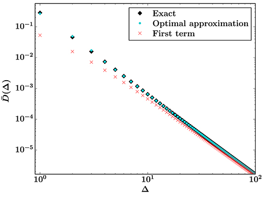
Figure 2. Optimal approximation from Equation (44) with 13 available terms (turquoise) and exact result (black) for the burst distribution. The first term of the asymptotic series (red), which is Equation (4), is shown for comparison. The threshold distribution is a Weibull distribution with k = 1 and t₀ = 0.

FIGURE 3

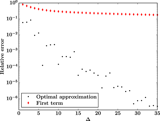
Figure 3. Relative errors for the burst distribution with respect to the exact result from Equation (14): for the optimal approximation from Equation (44) with 13 available terms (black) and for the first term of the asymptotic series (red), which is Equation (4). The threshold distribution is a Weibull distribution with k = 1 and t₀ = 0.

Both approximations converge to the exact solution as Δ → ∞, but the optimal approximation converges much faster and is consistently a better estimate of the exact result. From Figure 3, we see that the ratio between the two relative errors is at its smallest for small bursts, but the difference is still big, as evident from Figure 2. For the smallest bursts, the optimal approximation gives an estimate of the exact result with moderate accuracy (relative errors of order 10%), whereas Equation (4) is unusable as an estimate (relative errors of order 50% − 80%).

The errors in the optimal approximation seem to stem from the fact that 13 terms is insufficient to find the smallest term in the asymptotic series for small Δ. With 13 available terms, we can achieve higher accuracy with other parameters for the threshold distribution. For a Weibull distribution with k = 1 and t₀ = 0.8, we show the exact solution, optimal approximation, and Equation (4) in Figure 4, with the corresponding relative error of the optimal approximation in Figure 5.

FIGURE 4

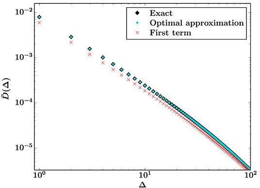
Figure 4. Optimal approximation from Equation (44) with 13 available terms (turquoise) and exact result (black) for the burst distribution. The first term of the asymptotic series (red), which is Equation (4), is shown for comparison. The threshold distribution is a Weibull distribution with k = 1 and t₀ = 0.8.

FIGURE 5

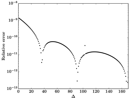
Figure 5. Relative error for the burst distribution with respect to the exact result from Equation (14) for the optimal approximation from Equation (44) (with 13 available terms). The threshold distribution is a Weibull distribution with k = 1 and t₀ = 0.8.

In this case, with t₀ = 0.8 much closer to x_c = 1, 13 terms seem to be sufficient to locate the smallest term in the asymptotic series even for small Δ. Hence the errors of the optimal approximation (of order 10⁻⁹ for the smallest bursts) are negligible, as seen from Figure 5. In the figure we have not shown the errors of Equation (4), since they are on a completely different scale from the errors of the optimal approximation, roughly 24% for the smallest bursts.

5.3. Comparison With Simulations

To test the general applicability of the asymptotic expansion, we also use Equation (44) with the uniform threshold distribution on [t₀, 1] (which has x_c = 1/2), a widely used probability distribution in the study of fiber bundles [3, 4]. Since the exact solution is valid only for Weibull distributions, we compare the asymptotic series results with simulation results for large systems (N = 1024²) where finite size effects for small Δ are small. As with the Weibull distributions, we again calculate the first 13 terms of Equation (31), and then use them to calculate the optimal approximation via Equation (44).

Figure 6 shows a comparison of the optimal approximation, simulation results, and Equation (4) for the uniform threshold distribution with t₀ = 0. The corresponding relative errors with respect to the simulation results, calculated as $|{\bar{D}}_{\mathrm{\text{simulation}}}-{\bar{D}}_{\mathrm{\text{approximation}}}|/{\bar{D}}_{\mathrm{\text{simulation}}}$, is shown in Figure 7. The optimal approximation is accurate to within a few percent for small bursts, and the relative error decreases rapidly as Δ increases, as in Figures 3, 5. However, the error quickly begins to increase again, presumably due to finite size effects from the simulations. Equation (31) is derived from Equation (5), which is only exact in the limit N → ∞. Equation (4) becomes more accurate as Δ increases, but is consistently less accurate than the optimal approximation.

FIGURE 6

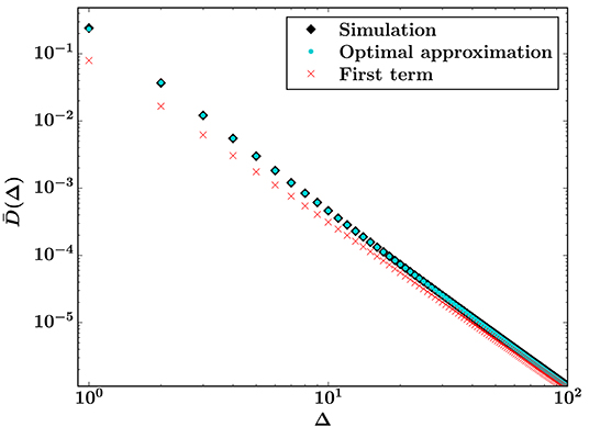
Figure 6. Optimal approximation from Equation (44) with 13 available terms (turquoise) and simulation results (black, N = 1024², 10⁶ samples) for the burst distribution. The first term of the asymptotic series (red), which is Equation (4), is shown for comparison. The threshold distribution is uniform on [0, 1].

FIGURE 7

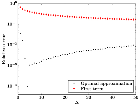
Figure 7. Relative errors for the burst distribution with respect to simulation results that are averaged over 10⁶ sample systems of size N = 1024²: for the optimal approximation from Equation (44) with 13 available terms (black) and for the first term of the asymptotic series (red), which is Equation (4). The threshold distribution is uniform on [0, 1].

Figure 8 shows a comparison of the optimal approximation, simulation results, and Equation (4) for the uniform threshold distribution with t₀ = 0.45, with corresponding relative errors in Figure 9. In this case neither approximation becomes more accurate as the burst size increases, but Equation (4) is much more accurate than for t₀ = 0. However, the optimal approximation is still more accurate than Equation (4), with relative errors roughly an order of magnitude smaller.

FIGURE 8

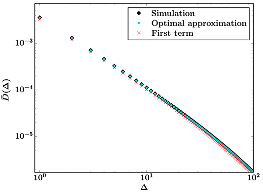
Figure 8. Optimal approximation from Equation (44) with 13 available terms (turquoise) and simulation results (black, N = 1024², 10⁶ samples) for the burst distribution. The first term of the asymptotic series (red), which is Equation (4), is shown for comparison. The threshold distribution is uniform on [0.45, 1].

FIGURE 9

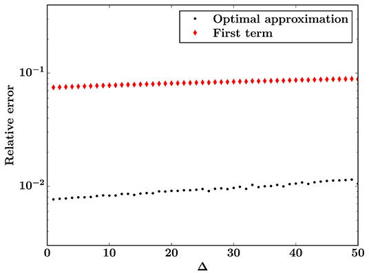
Figure 9. Relative errors for the burst distribution with respect to simulation results that are averaged over 10⁶ sample systems of size N = 1024²: for the optimal approximation from Equation (44) with 13 available terms (black) and for the first term of the asymptotic series (red), which is Equation (4). The threshold distribution is uniform on [0.45, 1].

6. Discussion and Conclusion

In the equal load sharing fiber bundle model, we have found an analytic solution of the burst size distribution for Weibull threshold distributions: Equation (14). This is a significant improvement over previous results, which describe the asymptotic behavior as the burst size diverges.

The exact result is impractical to use for large burst sizes Δ, but can easily be evaluated for small Δ. In this sense it complements the existing asymptotic result; Equation (14) can be used for small Δ, and for sufficiently large Δ we can use Equation (4) instead. Together, these results provide a highly accurate way to calculate the burst size distribution for Weibull threshold distributions.

For other threshold distributions where the burst distribution cannot be solved exactly, another method is needed to calculate the burst distribution for small Δ. We have therefore derived the full asymptotic series expansion for the burst size distribution, Equation (31). Even if the full infinite series is valid only in the limit Δ → ∞, it can still be used to find approximations for small Δ through Equation (44).

Our results indicate that, with a fixed number of available terms, this optimal approximation is more accurate the smaller x_c − t₀ is. This seems to stem, at least partially, from the fact that more terms are needed in the asymptotic series expansion to find the smallest term.

The accuracy of the optimal asymptotic approximation depends on the threshold distribution and the number of calculated terms. With 13 terms, the relative error for the smallest bursts ranges from several percent to ∼ 10⁻⁹ for the Weibull and uniform threshold distributions we have investigated. This is consistently more accurate than Equation (4).

Neither Equation (44) nor Equation (4) take finite size effects into account, since they are derived in the limit of infinitely big systems. The optimal approximation provides decent estimates of simulation results from large systems, when finite size effects are small, but the accuracy should be expected to be much smaller when comparing with results from small system sizes. It might be possible to use a similar approach that also incorporates finite size effects, but then one would first need to derive an expression like Equation (5) that contains the finite size effects.

Estimating the burst distribution via Equation (44) is much more computationally efficient than relying on simulations of very large systems. However, simulations can in theory give more accurate estimates, provided that the simulation results converge to the thermodynamic limit quickly enough when the system size increases. Then one can use results for different system sizes to extrapolate to N → ∞. Simulations should still be preferred when studying finite size effects, especially for small systems where simulations are not time-consuming. The optimal asymptotic approximation gives decent estimates for simulations results from large systems, as shown in Figures 7, 9, but we expect the accuracy to be smaller for smaller system sizes.

Data Availability Statement

The datasets generated for this study are available on request to the corresponding author.

Author Contributions

JK performed the research and wrote the manuscript.

Funding

This work was partly supported by the Research Council of Norway through its Centres of Excellence funding scheme, project number 262644.

Conflict of Interest

The author declares that the research was conducted in the absence of any commercial or financial relationships that could be construed as a potential conflict of interest.

Acknowledgments

I would like to thank Alex Hansen for suggesting to look for an exact solution, and for assisting with writing the abstract, introduction, and conclusion. I would also like to thank Martin Hendrick and Srutarshi Pradhan for helpful discussions and good suggestions.

References

1. Peirce FT. 32—X.—Tensile tests for cotton yarns v.—“The Weakest Link” Theorems on the strength of long and of composite specimens. J Text Inst. (1926) 17:T355–68. doi: 10.1080/19447027.1926.10599953

CrossRef Full Text

2. Daniels HE. The statistical theory of the strength of bundles of threads. I. Proc R Soc A. (1945) 183:405–35. doi: 10.1098/rspa.1945.0011

CrossRef Full Text | Google Scholar

3. Pradhan S, Hansen A, Chakrabarti BK. Failure processes in elastic fiber bundles. Rev Mod Phys. (2010) 82:499–555. doi: 10.1103/RevModPhys.82.499

CrossRef Full Text | Google Scholar

4. Hansen A, Hemmer PC, Pradhan S. The Fiber Bundle Model. Berlin: Wiley-VCH (2015).

Google Scholar

5. Bouchaud JP. Econophysics: still fringe after 30 years? Europhys News. (2019) 50:24–7. doi: 10.1051/epn/2019103

CrossRef Full Text | Google Scholar

6. Pradhan S, Hansen A, Hemmer PC. Crossover behavior in burst avalanches: signature of imminent failure. Phys Rev Lett. (2005) 95:125501. doi: 10.1103/PhysRevLett.95.125501

PubMed Abstract | CrossRef Full Text | Google Scholar

7. Pradhan S, Bhattacharyya P, Chakrabarti BK. Dynamic critical behavior of failure and plastic deformation in the random fiber bundle model. Phys Rev E. (2002) 66:016116. doi: 10.1103/PhysRevE.66.016116

PubMed Abstract | CrossRef Full Text | Google Scholar

8. Hemmer PC, Pradhan S. Failure avalanches in fiber bundles for discrete load increase. Phys Rev E. (2007) 75:046101. doi: 10.1103/PhysRevE.75.046101

PubMed Abstract | CrossRef Full Text | Google Scholar

9. Hemmer PC, Hansen A. The distribution of simultaneous fiber failures in fiber bundles. J Appl Mech. (1992) 59:909–14. doi: 10.1115/1.2894060

CrossRef Full Text | Google Scholar

10. Sornette D. Mean-field solution of a block-spring model of earthquakes. J Phys I. (1992) 2:2089–96. doi: 10.1051/jp1:1992269

CrossRef Full Text | Google Scholar

11. Pradhan S, Hansen A, Hemmer PC. Crossover behavior in failure avalanches. Phys Rev E. (2006) 74:016122. doi: 10.1103/PhysRevE.74.016122

PubMed Abstract | CrossRef Full Text | Google Scholar

12. Raischel F, Kun F, Herrmann HJ. Local load sharing fiber bundles with a lower cutoff of strength disorder. Phys Rev E. (2006) 74:035104. doi: 10.1103/PhysRevE.74.035104

PubMed Abstract | CrossRef Full Text | Google Scholar

13. Hidalgo RC, Moreno Y, Kun F, Herrmann HJ. Fracture model with variable range of interaction. Phys Rev E. (2002) 65:046148. doi: 10.1103/PhysRevE.65.046148

PubMed Abstract | CrossRef Full Text | Google Scholar

14. Bender CM, Orszag SA. Advanced Mathematical Methods for Scientists and Engineers: Asymptotic Methods and Perturbation Theory. New York, NY: Springer (1999).

Google Scholar