Langevin Dynamics Driven by a Telegraphic Active Noise

Self-propelled or active particles are referred to as the entities which exhibit anomalous transport violating the fluctuation-dissipation theorem by means of taking up an athermal energy source from the environment. Currently, a variety of active particles and their transport patterns have been quantified based on novel experimental tools such as single-particle tracking. However, the comprehensive theoretical understanding for these processes remains challenging. Effectively the stochastic dynamics of these active particles can be modeled as a Langevin dynamics driven by a particular class of active noise. In this work, we investigate the corresponding Langevin dynamics under a telegraphic active noise. By both analytical and computational approaches, we study in detail the transport and nonequilibrium properties of this process in terms of physical observables such as the velocity autocorrelation, heat current, and the mean squared displacement. It is shown that depending on the properties of the amplitude and duration time of the telegraphic noise various transport patterns emerge. Comparison with other active dynamics models such as the run-and-tumble and Lévy walks is also presented.

1. Introduction

Anomalous diffusion disobeying the fluctuation-dissipation theorem has been widely observed in active systems. Prominent examples are the motor-driven transport in living cells, crawling and swimming dynamics of a cell in free or confined space, the motion of artificial micro-swimmers like Janus particles, and the diffusion of an enzyme during catalysis [1–3]. It can be understood that these active dynamics, typically observed on a mesoscopic time & length scale, are collective phenomena resulted from complicated, myriad interactions among the components comprising the system in the presence of nonequilibrium energy sources. A currently attracting issue is to model the stochastic dynamics of individual active (self-propelled) particles at a coarse-grained level, in which a physical picture is that a single particle is immersed in an active bath, i.e., a heat bath in the presence of an extra nonequilibrium noise [4–8]. A closely connected issue to this problem in other fields is the study of quantifying superdiffusion in the complex (biological) systems [9]. Examples include the motor-driven transport of bio-materials in a cell [10, 11], the run-and-tumble motion of a bacterium [12], foraging motion of motile cells and animals [13], anomalous diffusion of ultracold atoms [14], and the dispersal of a banknote [15]. It has been shown that the displacement distributions often follow a (truncated) Lévy distribution and, thus, the models in the class of continuous-time random walks such as the Lévy flights and Lévy walks explain essential features of the observed stochastic dynamics [16]. In this description, the effect of the active or out-of-equilibrium noise is implicitly taken into account in the PDFs of displacement lengths and/or sojourn times.

In the above studies of the active anomalous diffusion, its stochastic dynamics is often modeled by the Langevin equation of the following form:

$\begin{array}{ll}m\stackrel{\cdot }{v}=-\gamma v+\xi (t)+f(t).& (1)\end{array}$

This equation describes the dynamics of a particle of mass m(= 1) in a viscous heat bath comprised of passive and active noises. ξ(t) is a thermal (gaussian) noise satisfying the zero mean (〈ξ〉 = 0) and the variance 〈ξ(t)ξ(t′)〉 = 2γβ⁻¹δ(t − t′) [γ: frictional coefficient, $\beta =1/k_B{T}$ the inverse temperature where k_B is the Boltzmann constant and ${T}$ is the absolute temperature]. The active noise f(t) is responsible for the nonequilibrium source in the system, of which statistical properties characterize the nature of active dynamics under consideration. Here, it is assumed that the two noises are independent each other such that the nonequilibrium environment caused by the active noise does not seriously change the characteristics of ξ(t). For a representative example, the tracer dynamics in an active bath containing E Coli micro-swimmers was modeled with the gaussian colored noise f_OU(t), often referred to as the Ornstein-Ulenbeck noise, characterized by 〈f_OU〉 = 0 and $\langle f_{\text{OU}}(t^{\prime })f_{\text{OU}}(t^{\prime }+t)\rangle \propto exp(-t/t_c)$ [17]. Regarding subdiffusive or superdiffusive dynamics of the particles embedded in a crowded, viscoelastic medium, their stochastic dynamics can be modeled with fractional gaussian noise f_H(t) [18] having a power-law decaying autocorrelation $\langle f_H(t^{\prime })f_H(t^{\prime }+t)\rangle \propto (2H-1)t^{-1+2H}$ with the Hurst exponent H (0 < H < 1) [19–23]. For animal or self-propelled particles (e.g., molecular-motor-driven cargo) exhibiting Lévy statistics, the f is a Lévy noise having the characteristics ${P}(f)\propto 1/f^{1+\mu }$ [24, 25].

In this work, we investigate the stochastic dynamics of single particles governed by Equation 1 with a telegraphic (i.e., step-like) noise f(t) as illustrated in Figure 1. Here the characteristics of the noise is described by its PDFs of noise amplitude ${P}(f)$ and of duration time P(τ). It is noted that by adjusting the PDFs P(τ) and ${P}(f)$ our nonequilibrium noise f(t) can become a shot-noise [26, 27] as well as a dichotomous noise [26, 28]. Hence, in general our model links these two distinct noises. Furthermore, we show that our model with P(τ) ~ 1/τ^1+α (0 < α < 2) serves a model for a Lévy walk superimposed with the thermal noise.

FIGURE 1

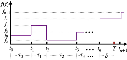
Figure 1. The schematic description of the telegraphic active noise f(t) considered in our Langevin equation 1. The protocol of the noise is given by f(t) = f_i for t ∈ [t_i, t_i+1], where the noise strength f_i and the duration time τ_i ≡ t_i+1 − t_i are random variables specifying the statistical properties of f(t). It is a renewal process such that the sequences of {f_i} and {τ_i} are i.i.d.s obtained from the PDF ${P}(f)$ and P(τ), respectively.

The current paper is organized as follows. In section 2 we present our path integral approach to solve the Langevin equation 1 with a telegraphic active force f(t). Dynamic quantities such as the velocity autocorrelation, heat rate, and the mean-square displacement (MSD) are derived in the underdamped level. Then we introduce the overdamped version of Equation 1 and investigate in detail the long-time dynamics of the particle. In section 3 complementary numerical study is provided. Here we generate the active force f(t) for a few distinct cases of P(τ) and simulate the corresponding Langevin equations. The results are compared and explained with the analytic studies in section 2. Lastly, in section 4, we summarize the main results with a discussion on the connection between our Langevin model and other active dynamics models.

2. Langevin Dynamics

In section 2 we analytically investigate the active dynamics of our Langevin model 1 under a telegraphic noise f(t). Prior to this, we briefly look at the autocorrelation property of f(t) and also introduce useful truncated statistics that used throughout the paper. In section 2.2 our path integral formalism to the Langevin equation 1 is presented with several analytic main results. In section 2.3 we propose the overdamped version of the original Langevin equation 1 and explicitly derive transport quantities for the three distinct types of f(t) (introduced in Table 1).

TABLE 1

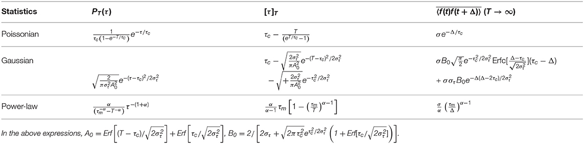
Table 1. The three duration time PDFs considered in our telegraphic noise f(t) and their statistical properties.

2.1. Noise Correlation of f(t)

A given time series of a telegraphic noise f(t) can be uniquely defined by its duration time sequence {τ_i} and the amplitude {f_i}, see Figure 1. First, let us consider the ensemble-averaged autocorrelation of f(t), denoted as 〈f(t)f(t + Δt)〉_{fi, τi}. In this expression, the symbol of 〈·〉_{fi, τi} represents the average over the active noise f(t) for the noise amplitudes f_i and the duration times τ_i. Since the PDFs ${P}(f)$ and P(τ) are independent, the corresponding two averages are independent. Exploiting this property, let us first calculate the f_i-averaged autocorrelation function 〈f(t)f(t+Δt)〉_fi for a given sequence {τ_i}. In this case, the corresponding active noise f(t)s have the same transition events, given by the {τ_i}, so that the number of transitions n until T is determined by the inequality $\sum _{i=0}^{n-1}{\tau }_i<T<\sum _{i=0}^n{\tau }_i$. For this set of f(t)s, the noise-amplitude averaged autocorrelation is given by

$\begin{array}{lll}{\langle f(t)f(t+\Delta t)\rangle }_{f_i}& =& \sigma {\displaystyle \sum _{i=0}^{n-1}}\Theta (t-t_i)\Theta (t_{i+1}-t-\Delta t)\\ & & +\sigma \Theta (t-t_n)\Theta (T-t-\Delta t)& (2)\end{array}$

where Θ(x) is the Heaviside step function [Θ(x) = 1 for x > 0, otherwise zero] and 〈f_lf_m〉f_i = σδ_lm is used.

To get the full ensemble-averaged autocorrelation, one has to average Equation 2 over all possible sequences of {τ_i}. This average can be effectively obtained by performing the time average of Equation 2 with an assumption that T is sufficiently large enough to have many transition events (n is large). For nonequilibrium systems this ergodic relation may not be generally guaranteed [1, 4, 29], but we have numerically confirmed this for the telegraphic active noises investigated in this study. We leave the ergodicity test and further discussions in the Appendix A2.C. Accordingly, we obtain the expression

$\begin{array}{lll}\overline{{\langle f(t)f(t+\Delta t)\rangle }_{f_i}}& =& \frac{\sigma }{T-\Delta t}{\displaystyle {\int }_0^{T-\Delta t}}dt{\langle f(t)f(t+\Delta t)\rangle }_{f_i},\\ & =& \frac{\sigma }{T-\Delta t}[{\displaystyle \sum _{i=0}^{n-1}}({\tau }_i-\Delta t)\Theta ({\tau }_i-\Delta t)\\ & & +(\eta -\Delta t)\Theta (\eta -\Delta t)],& (3)\end{array}$

where $\eta =T-\sum _{i=0}^{n-1}{\tau }_i$. To evaluate the finite summation in the above expression, we define the average number of events N(≫1) in the time window [0, T] where N = T/[τ]_T and [τ]_T is the mean duration time of τ_i in [0, T], given by the self-consistent equation

$\begin{array}{ll}{\left[\tau \right]}_T={\displaystyle {\int }_0^T}d\tau \tau P_T(\tau ).& (4)\end{array}$

Here, P_T(τ) is the truncated PDF defined in the interval [0, T] from the original one P(τ), i.e., $P_T(\tau )=P(\tau )/\left[{\int }_0^{T}d\tau P(\tau )\right]$. Note that N (or n) is large, so we are allowed to replace the summation in Equation 3 by $\frac{1}{n}\sum _{i=0}^{n-1}\to {\int }_0^{T}d\tau P_T(\tau ).$ Then, using n ≈ N and Δt/[τ]_T ≪ N, we obtain the time-averaged autocorrelation function

$\begin{array}{ll}\overline{{\langle f(t)f(t+\Delta t)\rangle }_{f_i}}=\frac{\sigma }{{\left[\tau \right]}_T}{\displaystyle {\int }_{\Delta t}^T}d\tau (\tau -\Delta t)P_T(\tau ).& (5)\end{array}$

For the definition and the autocorrelation properties of the three types of f(t) considered in this work, refer to Table 1. It is noted that the time-averaged expression 5 is valid and fulfills ergodicity since the duration time PDF of f(t) in our study has a finite mean. Our study below is restricted to this case.

2.2. Path Integral Formalism and the Underdamped Langevin Dynamics

Analogously to section 2.1, let us start to solve the Langevin equation 1 with f(t) observed in [0, T] under the condition that the sequences of {f_i} and {τ_i} were predetermined.

First, consider the particle dynamics for an infinitesimal time interval δt(≪1) during which the f(t) is a constant. In this case, according to Onsager and Machlup [30], the propagator of v is given by

$\begin{array}{ll}\Pi \left[v^{\prime }|v\right]=\sqrt{\frac{\beta }{4\pi \gamma \delta t}}\text{ exp }\left[-\frac{{\left(v^{\prime }-v+\gamma v\delta t-f_i\delta t\right)}^2}{4\gamma {\beta }^{-1}\delta t}\right]& (6)\end{array}$

where v = v(t), v′ = v(t + δt), and f(t) = f_i. Next, we look for the propagator Π of v(t) and v(t + Δt) for an arbitrary time interval Δt during which f(t) is allowed to have multiple transitions. With a given f(t), it can be shown that the propagator is written as [31]

$\begin{array}{ll}\Pi \left[v^{\prime }|v\right]=\sqrt{\frac{\beta }{2\pi w(\Delta t)}}\text{ exp }\left[-\frac{{\left(v^{\prime }-e^{-\gamma \Delta t}v-\lambda (t^{\prime },t)\right)}^2}{2{\beta }^{-1}w(\Delta t)}\right]& (7)\end{array}$

where w(Δt) = (1 − e^−2γΔt) and λ(t′, t) is the convolution integral of f(t), given by

$\begin{array}{ll}\lambda (t^{\prime },t)={\displaystyle {\int }_t^{t^{\prime }}}ds{e}^{-\gamma (t^{\prime }-s)}f(s).& (8)\end{array}$

The derivation of Equation 7 is described in the Appendix A1. For example, when t_i < t < t_i+1 and $t_j<t^{\prime }<t_{j+1}$ (i < j), λ(t′, t) reads

$\begin{array}{lll}\lambda (t^{\prime },t)& =& {\lambda }_i(t)e^{-\gamma (t^{\prime }-t_{i+1})}+e^{-\gamma (t^{\prime }-t_j)}{\displaystyle \sum _{k=i+1}^{j-1}}{\lambda }_k{\displaystyle \prod _{l=k+1}^{j-1}}{e}^{-\gamma {\tau }_l}\\ & & +\frac{f_j}{\gamma }\left(1-e^{-\gamma (t^{\prime }-t_j)}\right),& (9)\end{array}$

where λ_k = λ_k(t_k) is given by

$\begin{array}{ll}{\lambda }_k=\frac{f_k}{\gamma }\left(1-e^{-\gamma (t_{k+1}-t_k)}\right)=\frac{f_k}{\gamma }\left(1-e^{-\gamma {\tau }_k}\right)& (10)\end{array}$

and ${\lambda }_i(t)=\frac{f_i}{\gamma }\left(1-e^{-\gamma (t_{i+1}-t)}\right)$. If f(t) has no transition event in [t, t′] where $t_i<t<t^{\prime }<t_{i+1}$, Equation 9 is reduced to $\lambda (t^{\prime },t)=\frac{f_i}{\gamma }\left(1-e^{-\gamma (t^{\prime }-t)}\right).$ Given λ(t, t₀), the conditional PDF of v is similarly obtained with the initial condition p(v₀|λ) = δ(v₀) as

$\begin{array}{ll}p\left(v|\lambda (t,t_0)\right)=\sqrt{\frac{\beta }{2\pi w(t-t_0)}}\text{ exp }\left[-\frac{{\left(v-\lambda (t,t_0)\right)}^2}{2{\beta }^{-1}w(t-t_0)}\right].& (11)\end{array}$

Heat is defined as the energy gain from a heat bath to the particle. Heat rate is given by [32]

$\begin{array}{ll}\stackrel{\cdot }{Q}=-(-\gamma v+\xi )◦v,& (12)\end{array}$

where ◦ denotes the Stratonovich calculus. Using $(-\gamma v+\xi )◦v=(-\gamma v+\xi )(v+(1/2)\stackrel{\cdot }{v}dt)$ and averaging over the thermal noise, we obtain the conditional heat rate, ${\langle \stackrel{\cdot }{Q}\rangle }_{\xi }$, where 〈·〉_ξ stands for the thermal average over ξ for given protocol f(t),

$\begin{array}{ll}{\langle \stackrel{\cdot }{Q}\rangle }_{\xi }=\gamma {\langle v^2\rangle }_{\xi }-\frac{1}{2}{\langle {\xi }^2\rangle }_{\xi }dt=\gamma \left({\langle v^2\rangle }_{\xi }-{\beta }^{-1}\right).& (13)\end{array}$

Here, the equal-time correlation function in Equation 13 is given by ${\langle v^2\rangle }_{\xi }=\int dv{v}^{2}p(v|\lambda (t,t_0))$, which reads

$\begin{array}{ll}{\langle v^2(t)\rangle }_{\xi }={\beta }^{-1}w(t-t_0)+{\left[\lambda (t,t_0)\right]}^2.& (14)\end{array}$

In R.H.S, the first term explains the relaxation kinetics toward thermal equilibrium and the second term describes the energy input from the active force f(t). In the limit of t → ∞, w(t − t₀) → 1 at which the heat rate ${\langle \stackrel{\cdot }{Q}\rangle }_{\xi }$ becomes $\gamma {\left[\lambda (t,t_0)\right]}^2$.

The average over the noise amplitude (f_i) can be further evaluated on the condition that the sequence {τ_i} is quenched. About the active force term ${\lambda }^2(t,t_0)$, its averaged quantity over ${P}(f)$ is calculated to

$\begin{array}{lll}{\langle {\left[\lambda (t,t_0)\right]}^2\rangle }_{\xi ,f_i}& =& \frac{\sigma }{{\gamma }^2}{e}^{-2\gamma (t-t_i)}{\displaystyle \sum _{k=0}^{i-1}{\left(1-e^{-\gamma {\tau }_k}\right)}^2}{\displaystyle \prod _{l=k+1}^{i-1}{e}^{-2\gamma {\tau }_l}}\\ & & +\frac{\sigma }{{\gamma }^2}{\left(1-e^{-\gamma (t-t_i)}\right)}^2,& (15)\end{array}$

where the index i represents the transition time (of f(t)) specifying t_i < t < t_i+1. The notation 〈·〉_ξ,fi denotes the average over both the thermal noise ξ(t) and the amplitude f_i of f(t), henceforth. From this relation, we identify that the averaged heat rate has the relation

$\begin{array}{ll}{\langle \stackrel{\cdot }{Q}(t\to \infty )\rangle }_{\xi ,f_i}={\displaystyle \underset{t\to \infty }{\text{lim}}}\gamma {\langle {\left[\lambda (t,t_0)\right]}^2\rangle }_{\xi ,f_i}.& (16)\end{array}$

This relation tells that the system has a non-vanishing heat rate (at t → ∞) from the telegraphic noise; it acts as a non-conservative force to the system, driving the particle out of equilibrium constantly and leading to a non-vanishing heat rate. According to Equation 15, however, there is an exceptional case where the heat rate can be vanishing. This happens in the limit of [τ]_T → 0 where all the exponential terms in Equation 15 are unity (τ_k, τ_l, and t − t_i go to zero). In this case, the telegraphic noise is no longer telegraphic and the effect of f(t) to the system is negligible compared to the thermal noise.

Using Equation 15, the noise-amplitude averaged v² is given by

$\begin{array}{ll}{\langle v^2(t)\rangle }_{\xi ,f_i}={\beta }^{-1}w(t-t_0)+{\langle {\left[\lambda (t,t_0)\right]}^2\rangle }_{\xi ,f_i}.& (17)\end{array}$

As time is increased to infinity, both terms of w(t − t₀) and ${\lambda }^2(t,t_0)$ decay out and v² reaches a stationary value. This value can be evaluated in the limit of t − t₀ → ∞ where, in Equation 15, τ_i in the exponential terms are approximated to [τ]_T, yielding $\sum _{k=0}^{i-1}{\left(1-e^{-\gamma {\tau }_k}\right)}^2{\prod }_{l=k+1}^{i-1}{e}^{-2\gamma {\tau }_l}\approx {\left(1-e^{-\gamma {\left[\tau \right]}_T}\right)}^2\sum _{k=0}^{\infty }{e}^{-2k\gamma {\left[\tau \right]}_T}=(1-e^{-\gamma {\left[\tau \right]}_T})/(1+e^{-\gamma {\left[\tau \right]}_T}).$ Subsequently, we further perform the average over the duration time {τ_i} by way of time-averaging and finally obtain the time-averaged $\overline{{\langle v^2\rangle }_{\xi ,f_i}}$ at t → ∞

$\begin{array}{ll}\overline{{\langle v^2\rangle }_{\xi ,f_i}}={\beta }^{-1}+\frac{\sigma }{{\gamma }^2}\left(1-\frac{1-e^{-\gamma {\left[\tau \right]}_T}}{\gamma {\left[\tau \right]}_T}\right).& (18)\end{array}$

This result will be confirmed in section 3 by the numerical study.

Velocity autocorrelation function (VACF) for v = v(t) and v′ = v(t + Δt) for a given f(t) can be obtained from the propagator (Equation 7), which is

$\begin{array}{ll}{\langle v{v}^{\prime }\rangle }_{\xi }=e^{-\gamma \Delta t}{\langle v^2\rangle }_{\xi }+\lambda (t^{\prime },t)\lambda (t,t_0).& (19)\end{array}$

The noise-amplitude averaged VACF is then found to be

$\begin{array}{lll}{\langle v^{\prime }v\rangle }_{\xi ,f_i}& =& e^{-\gamma \Delta t}[{\beta }^{-1}w(t-t_0)\\ & & +{\langle {\left[\lambda (t,t_0)\right]}^2\rangle }_{\xi ,f_i}]+{\langle \lambda (t^{\prime },t)\lambda (t,t_0)\rangle }_{\xi ,f_i}& (20)\end{array}$

where $\langle \lambda (t^{\prime },t)\lambda (t,t_0)\rangle$ means

$\begin{array}{ll}{\langle \lambda (t^{\prime },t)\lambda (t,t_0)\rangle }_{\xi ,f_i}=\frac{\sigma }{{\gamma }^2}{e}^{-\gamma (t^{\prime }-t_{i+1})}\left(1-e^{-\gamma (t_{i+1}-t)}\right)\left(1-e^{-\gamma (t-t_i)}\right)& (21)\end{array}$

for $t_i<t<t_{i+1}<t^{\prime }$ and

$\begin{array}{ll}{\langle \lambda (t^{\prime },t)\lambda (t,t_0)\rangle }_{\xi ,f_i}=\frac{\sigma }{{\gamma }^2}\left(1-e^{-\gamma (t^{\prime }-t)}\right)\left(1-e^{-\gamma (t-t_i)}\right)& (22)\end{array}$

for $t_i<t<t^{\prime }<t_{i+1}$.

The mean squared displacement (MSD) of the particle in the interval [t, t + Δt] can be obtained via the double integral of VACF

$\begin{array}{ll}{\langle {\left[\Delta x(\Delta t;t)\right]}^2\rangle }_{\xi ,f_i}={\displaystyle {\int }_t^{t+\Delta t}}ds{\displaystyle {\int }_t^{t+\Delta t}}du{\langle v(s)v(u)\rangle }_{\xi ,f_i}.& (23)\end{array}$

Within a short time interval Δt ≪ 1, Equation 23 can be expanded to

$\begin{array}{ll}{\langle \Delta x^2\rangle }_{\xi ,f_i}\approx {{\displaystyle \langle }{\left(\frac{v(t)+v(t+\Delta t)}{2}\right)}^2{\displaystyle \rangle }}_{\xi ,f_i}\Delta t^2.& (24)\end{array}$

Using $\left[v(t)+v(t+\Delta t)\right]/2\approx v+\stackrel{\cdot }{v}\Delta t/2$, we obtain the MSD up to the next leading order,

$\begin{array}{ll}{\langle \Delta x^2\rangle }_{\xi ,f_i}& \approx {\langle v^2\rangle }_{\xi ,f_i}\Delta t^2\\ & +\left[\frac{{\langle \lambda (t,t_0)f(t)\rangle }_{\xi ,f_i}}{2}+\gamma {\beta }^{-1}-\gamma {\langle v^2\rangle }_{\xi ,f_i}\right]\Delta t^3.& (25)\end{array}$

This result suggests that the MSD always starts to grow ballistically in the beginning where the amplitude ${\langle v^2\rangle }_{\xi ,f_i}$ is given by Equation 18.

For the other extreme limit of Δt → ∞ together with t ≫ t₀, we find that up to the order of 1/γ³ the MSD, Equation 23, grows with Δt in the form of

$\begin{array}{ll}{\langle \Delta x^2\rangle }_{\xi ,f_i}\approx \frac{2{\beta }^{-1}}{\gamma }\Delta t-\frac{2{\beta }^{-1}}{{\gamma }^2}+\frac{\sigma }{{\gamma }^2}{\displaystyle \sum _{i=1}^n}\left[{\tau }_i^2+\frac{4{\tau }_i}{\gamma }{e}^{-\gamma {\tau }_i}\right].& (26)\end{array}$

Here, the boundary terms are neglected and n is the number of events in [t, t + Δt]. This is the expression for a quenched sequence of {τ_i}. Equation 26 suggests that in the long-time limit where Δt ≫ γ⁻¹ (which is the momentum relaxation time m/γ) the MSD dynamics is eventually determined by the first linear term (thermal) and the sum of ${\tau }_i^2$ (active). The active part term can be reasonably rewritten as $\sum _{i=1}^n{\tau }_i^2\to n{\left[{\tau }^2\right]}_T\approx \left({\left[{\tau }^2\right]}_T/{\left[\tau \right]}_T\right)\Delta t$. Therefore, the second moment of duration time plays a crucial role in the long-time transport. Further development will be presented in the following section 2.3.

Equation 26 also suggests that the long-time limit dynamics of our underdamped Langevin model can be alternatively obtained by taking the overdamped limit: γ → ∞ (or m/γ → 0) while 1/[βγ] and σ/γ² keep finite. It is shown below that the MSD Equation 26 in this limit is identical to the MSD (Equation 35) of the overdamped version of the original underdamped Langevin equation 1. In the following section, we introduce this overdamped Langevin equation and investigate its MSD dynamics in a precise manner.

2.3. Overdamped Limit

Using the rescaled noises, $\tilde{\xi }=\xi /\gamma$ and $\tilde{f}(t)=f(t)/\gamma$, from our Langevin equation 1 we obtain the equation of motion for the overdamped dynamics as such

$\begin{array}{ll}\dot{x}=\tilde{\xi }+\tilde{f}(t),& (27)\end{array}$

where the gaussian white noise has the autocorrelation property $\langle \tilde{\xi }(t)\tilde{\xi }(t^{\prime })\rangle =2D\delta (t-t^{\prime })$ with D = β⁻¹/γ. Akin to the v(t) in the underdamped case, when the time series of $\tilde{f}(t)$ is given, the PDF for x(t) is evaluated to

$\begin{array}{ll}p\left(x|\tilde{\lambda }(t,t_0)\right)=\sqrt{\frac{1}{4\pi Dt}}\text{ exp }\left[-\frac{{\left(x-\stackrel{\text{~}}{\lambda }(t,t_0)\right)}^2}{4Dt}\right],& (28)\end{array}$

where x(t₀) = 0 and

$\begin{array}{ll}\tilde{\lambda }(t,t_0)={\displaystyle {\int }_{t_0}^t}ds\tilde{f}(s).& (29)\end{array}$

Therefore, $\tilde{\lambda }(t,t_0)$ means the mean drifted distance for given f(t) and the PDF of x(t) is a gaussian distribution centered at $\tilde{\lambda }(t,t_0)$. However, the noise-averaged PDF of x has a complicated structure beyond the simple gaussian. This will be discussed with the simulation in the next section. In the special case where $P(\tau )=e^{-\tau /{\tau }_c}/{\tau }_c$ and the two-state amplitude ${P}(\tilde{f})=\frac{1}{2}\delta (\tilde{f}-{\tilde{f}}_0)+\frac{1}{2}\delta (\tilde{f}+{\tilde{f}}_0)$, $\tilde{f}(t)$ can be treated as a dichotomous noise switching between the two states with a constant transition rate ${(2{\tau }_c)}^{-1}$. This model was analytically studied in a recent work [33] within the approach using a generalized telegrapher's equation.

In the limit of γ/m ≫ 1 (while 1/[βγ] and σ/γ² are finite), we find that the heat rate ${\langle \stackrel{\cdot }{Q}\rangle }_{\xi ,f_i}$ in Equation 16 is reduced to ${\langle \stackrel{\cdot }{Q}\rangle }_{\xi ,f_i}=\gamma \tilde{\sigma }$. The same conclusion is drawn from the overdamped equation, Equation 27, yielding

$\begin{array}{ll}{\langle \stackrel{\cdot }{Q}\rangle }_{\tilde{\xi },{\tilde{f}}_i}={{\displaystyle \langle }\left(\gamma \dot{x}-\gamma \tilde{\xi }\right)◦\dot{x}{\displaystyle \rangle }}_{\tilde{\xi },{\tilde{f}}_i}=\gamma \tilde{\sigma }& (30)\end{array}$

where ${\langle ·\rangle }_{\tilde{\xi },{\tilde{f}}_i}$ denotes the double average over the thermal noise $\tilde{\xi }$ and the amplitude ${\tilde{f}}_i$ of the active noise $\tilde{f}(t)$. The PDF Equation 28 tells that the MSD is given by

$\begin{array}{ll}{\langle \Delta x^2(\Delta t;t)\rangle }_{\tilde{\xi }}=2D\Delta t+{\left[\tilde{\lambda }(t^{\prime },t)\right]}^2,& (31)\end{array}$

where t′ = t + Δt. By performing the average of Equation 31 over the noise amplitude ${P}(f)$, we obtain

$\begin{array}{ll}{\langle \Delta x^2\rangle }_{\tilde{\xi },{\tilde{f}}_i}=2D\Delta t+\tilde{\sigma }\left[{(t^{\prime }-t_j)}^2+{\displaystyle \sum _{k=i+1}^{j-1}}{\tau }_k^2+{(t_{i+1}-t)}^2\right]& (32)\end{array}$

where t_i < t < t_i+1 and $t_j<t^{\prime }<t_{j+1}(i<j)$; for t_i = t_j, ${\langle \Delta x^2\rangle }_{\tilde{\xi },{\tilde{f}}_i}=2D\Delta t+\tilde{\sigma }\Delta t^2$.

From Equation 32, we finally find the analytic form of MSD averaged over the noise duration time with P(τ). Direct evaluation of the τ-average on Equation 32 is, however, not straightforward. In this work, we obtain this average by self-averaging Equation 32 over time at the large-T limit. This task is essentially same as finding the time-averaged MSD of Equation 32

$\begin{array}{ll}\overline{{\langle \Delta x^2\rangle }_{\tilde{\xi },{\tilde{f}}_i}}=\frac{1}{T-\Delta t}{\displaystyle {\int }_0^{T-\Delta t}}dt{\langle {\left[\Delta x(\Delta t;t)\right]}^2\rangle }_{\tilde{\xi },{\tilde{f}}_i}.& (33)\end{array}$

To calculate this, we follow the trick used in finding the autocorrelation of f(t). Consider a sequence {τ₀, …, τ_n} where n is the last event satisfying $\sum _{i=0}^{n-1}{\tau }_i<T<\sum _{i=0}^n{\tau }_i$. In the assumption of periodic B.C. (where the sequence of τ_i in [0, Δt] appears again in [T − Δt, T]), we find that Equation 33 is evaluated to

$\begin{array}{lll}\overline{{\langle \Delta x^2\rangle }_{\tilde{\xi },{\tilde{f}}_i}}& \equiv & \overline{\langle \Delta x^2\rangle }=2D\Delta t+\frac{\tilde{\sigma }}{T-\Delta t}[{\displaystyle \sum _{{\tau }_i<\Delta t}}\left({\tau }_i^2\Delta t-\frac{{\tau }_i^3}{3}\right)\\ & & +{\displaystyle \sum _{{\tau }_i>\Delta t}}\left({\tau }_i\Delta t^2-\frac{\Delta t^3}{3}\right)].& (34)\end{array}$

From now on, for simplicity, we drop the subscript $\tilde{\xi },{\tilde{f}}_i$ in expressing the multiple average of $\overline{{\langle ·\rangle }_{\tilde{\xi },{\tilde{f}}_i}}$. In the long observation time limit where n ≫ 1, the statistics is sufficient enough so as to replace the summation above by integral with the truncated PDF P_T(τ) defined in [0, T], see Table 1. Using this, we obtain the expression of the fully averaged MSD in terms of P_T(τ) as

$\begin{array}{lll}\overline{\langle \Delta x^2\rangle }& =& 2D\Delta t+\frac{\tilde{\sigma }}{{\left[\tau \right]}_T}[{\displaystyle {\int }_0^{\Delta t}}d\tau P_T(\tau )\left({\tau }^2\Delta t-\frac{{\tau }^3}{3}\right)\\ & & +{\displaystyle {\int }_{\Delta t}^T}d\tau P_T(\tau )\left(\tau \Delta t^2-\frac{\Delta t^3}{3}\right)]& (35)\end{array}$

where ${\left[\tau \right]}_T={\int }_0^{T}d\tau \tau P_T(\tau )$ is the average duration time observed in [0, T].

2.3.1. Poissonian and Gaussian PDFs

Plugging the corresponding P_T(τ)s in Table 1 into Equation 35 we can in principle obtain the explicit form of the time-averaged MSDs (not shown). For P(τ)s having a well-defined time scale τ_s( ~ [τ]_T), the MSD is shown to have the following universal structures at the two extreme time scales:

$\begin{array}{ll}\overline{\langle \Delta x^2\rangle }\approx \{\begin{array}{cc}2D\Delta t+\tilde{\sigma }\Delta t^2-\frac{\tilde{\sigma }}{3{\left[\tau \right]}_T}\Delta t^3,& \Delta t\ll {\tau }_s\\ 2D\Delta t+\frac{\tilde{\sigma }{\left[{\tau }^2\right]}_T}{{\left[\tau \right]}_T}\Delta t-\frac{\tilde{\sigma }{\left[{\tau }^3\right]}_T}{3{\left[\tau \right]}_T},& \Delta t\gg {\tau }_s\end{array}.& (36)\end{array}$

The result suggests that the overdamped dynamics have the Fickian behavior at both limiting time scales, with different diffusivities. For Δt ≪ τ_s, the active noise effects negligibly, where the particle has the bare diffusivity D. For the opposite limit of Δt ≫ τ_s, the particle ultimately attains a larger Fickian transport with an apparent diffusivity

$\begin{array}{ll}{D}_L=D+\frac{\tilde{\sigma }{\left[{\tau }^2\right]}_T}{2{\left[\tau \right]}_T}.& (37)\end{array}$

Detailed information about the profile of P(τ) is irrelevant for the nature of long-time transport; it only affects D_L through the first and second moments of the duration time. An example belonging to this class is the two-state active system with a constant transition rate ${(2{\tau }_c)}^{-1}$ introduced in Malakar et al. [33]. This system can be modeled in our Langevin description with $P(\tau )={\tau }_c^{-1}{e}^{-\tau /{\tau }_c}$ and ${\tilde{f}}_i=\pm {\tilde{f}}_0$. For this model, we analytically evaluate the MSD 35 with T → ∞ and obtain the identical form of MSD reported in Malakar et al. [33]

$\begin{array}{ll}\overline{\langle \Delta x^2\rangle }=2(D+{\tau }_c{\tilde{f}}_0^2)\Delta t-2{\tau }_c^2{\tilde{f}}_0^2(1-e^{-\Delta t/{\tau }_c}).& (38)\end{array}$

This expression shows that, for Δt ≪ τ_c, $\overline{\langle \Delta x^2\rangle }=2D\Delta t+{\tilde{f}}_0^2\Delta t^2-\frac{{\tilde{f}}_0^2}{3{\tau }_c}\Delta t^3$ while, for Δt ≫ τ_c, $\overline{\langle \Delta x^2\rangle }=2(D+{\tau }_c{\tilde{f}}_0^2)\Delta t-2{\tau }_c^2{\tilde{f}}_0^2$ where the apparent diffusivity is $D+{\tau }_c{\tilde{f}}_0^2$. These results are reproduced by plugging ${\left[{\tau }^q\right]}_{T\to \infty }={\tau }_c^{-1}{\int }_0^{\infty }{\tau }^q{e}^{-t/{\tau }_c}$ into Equations 36 and 37.

2.3.2. Power-Law PDFs

Considering $P_T(\tau )\propto {\tau }^{-1-\alpha }$ in [τ_m, T], the finite-time expectations, [τ]_T and ${\left[{\tau }^2\right]}_T$, are obtained in terms of α, T, and τ_m (Table 1). For the large-time limit of Δt → ∞, we obtain the asymptotic scaling relations of MSD depending on α:

$\begin{array}{ll}\overline{\langle \Delta x^2\rangle }\approx \{\begin{array}{cc}{a}_1+a_2\Delta t^{\alpha }+a_3\Delta t+a_4\Delta t^2,& 0<\alpha \le 1\\ b_1+b_2\Delta t+b_3\Delta t^{3-\alpha },& 1<\alpha \le 2\\ c_1+c_2\Delta t^{3-\alpha }+c_3\Delta t,& 2<\alpha \le 3\\ d_1+d_2\Delta t,& 3<\alpha \end{array}.& (39)\end{array}$

Here, {a_i}, {b_i}, {c_i}, and {d_i} are constants expressed with α, D, and other time constants (we omit providing these lengthy expressions except for c₃ = d₂ = 2D_L). The above expression explains that the long-time motion is akin to that of the Lévy walk [9], sensitively depending on the value of α. For a heavy-tailed PDF of a diverging mean ${\left[\tau \right]}_T~T^{1-\alpha }$ (0 < α < 1), the ballistic dynamics dominates over the other corrections as Δt approaches to T. For 1 < α ≤ 2, the mean duration time is finite ([τ]_T = ατ_m/(α − 1)), but the second moment is diverging (${\left[{\tau }^2\right]}_T~T^{2-\alpha }$). In this case, the long-time dynamics is ultimately governed by the sub-ballistic superdiffusion term of Δt^3−α. These superdiffusive dynamics in the range of α between 0 and 2 can emerge for a particle in a fluid in the hydrodynamic regime [9, 34, 35]. For all α > 2, the first and second moments of τ are all finite, which, thus, results in the Fickian long-time dynamics (~Δt) as in the cases of poissonian and gaussian PDFs. In this case, the long-time diffusivity D_L has exactly the same expression in Equation 37. As a special case, for α in between 2 and 3, the divergence of ${\left[{\tau }^3\right]}_T$ gives the nonvanishing correction term $c_2\Delta t^{3-\alpha }$ (see Equation 36); however, this term is sublinear and negligible compared to the Fickian term Δt at large times.

3. Numerical Results

In this section, we perform the Langevin dynamics simulation of Equation 1 and elucidate the transport dynamics with the theoretical expectations presented in the previous section. In our simulation study, we consider the three distinct f(t) governed by P(τ) of a poissonian, gaussian, and of a power-law, respectively. The specific functional form of these PDFs used in our study is presented in Table 1, with information about their autocorrelation properties. Figure 2 shows sample time series of f(t) generated in our simulation where the noise amplitude was chosen from a uniform ${P}(f)$ in the interval [−f₀, f₀] for all simulations, otherwise specified. Further information on the simulation procedure is provided in the Appendices A2, A3.

FIGURE 2

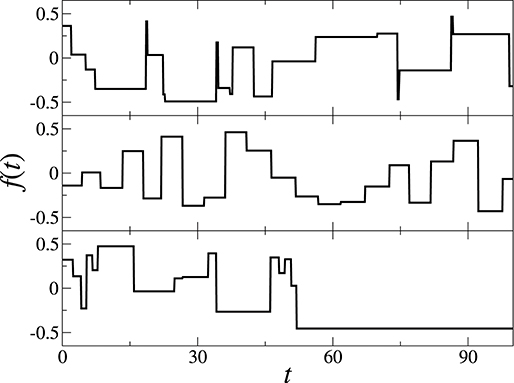
Figure 2. Time trace of the telegraphic noise f(t) generated in simulation. From Top to Bottom the sample noise was generated from the duration time PDFs: poissonian $P(\tau )\propto e^{-\tau /{\tau }_c}$, gaussian $P(\tau )\propto e^{-{(\tau -{\tau }_c)}^2/2{\sigma }_{\tau }^2}$, and power-lawed P(τ) ∝ τ^−(1+α). The parameters we used are τ_c = 5, σ_τ = 0.5, α = 1.2, and the unit time step 0.01, which gives the theoretical values for ${\left[\tau \right]}_{T\to \infty }(\equiv {\int }_0^{T\to \infty }d\tau \tau P(\tau ))=5$ (poissonian, gaussian) and 6 (power-law). The noise strength f_i was chosen from a uniform distribution in the interval of [−0.5, 0.5].

3.1. Dynamics of v²(t)

In Figure 3 we plot the relaxation of ${\langle v^2(t)\rangle }_{\xi ,f_i,{\tau }_i}$ (black) from 10⁵ sample trajectories of the Langevin equation 1 for the three distinct f(t) (see the Caption for further information). Here, in simulation, the full ensemble-averaged v², ${\langle v^2(t)\rangle }_{\xi ,f_i,{\tau }_i}$, is evaluated via the average over the thermal noise as well as the amplitude and duration time of f(t).The data is compared with the theoretical curve (red) of ${\langle v^2(t)\rangle }_{\xi ,f_i,{\tau }_i}$, which is computationally obtained from Equation (17) with the average over {τ_i}. The stationary value of ${\langle v^2(t\to \infty )\rangle }_{\xi ,f_i,{\tau }_i}$ is approximately given by Equation 18 (blue). For all cases, the data are excellently explained by our analytical counterparts.

FIGURE 3

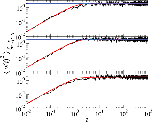
Figure 3. Relaxation dynamics of ${\langle v^2(t)\rangle }_{\xi ,f_i,{\tau }_i}$. From Top to Bottom they are the cases with f(t) of a poissonian, gaussian, and a power-law P(τ), respectively. The simulation data (black) were obtained by solving the Langevin Equation 1 with timestep δt = 0.01, v₀ = 0, and the total observation window T = 2000. Two theoretical lines are compared to the data: ${\langle v^2(t)\rangle }_{\xi ,f_i,{\tau }_i}$ (red) obtained from Equation 17 with the additional numerical average over {τ_i} and the stationary value (blue) Equation 18. In the simulation, we used the parameters: m = β = γ = 1, τ_c = 10 and σ_τ = 1 for the poissonian and gaussian PDFs, and α = 1.2 (producing [τ]_T = 5.7) for the power-law PDF. For all cases, ${P}(f)$ is a uniform distribution in $\left[-\sqrt{3},\sqrt{3}\right]$. The units in our Langevin simulation of Equation 1 are: $\left[x\right]=1/\sqrt{\beta \sigma }$, $\left[t\right]=\sqrt{m/(\beta \sigma )}$.

3.2. MSD

In Figure 4 we plot the full ensemble-averaged MSDs over random realizations of the noise strength {f_i} as well as the duration time {τ_i} for the three cases of f. At the underdamped timescale, as predicted in Equation 25, the MSDs have the ballistic scaling with the same amplitude for all cases. We confirm that this amplitude corresponds to $\overline{{\langle v^2\rangle }_{\xi ,f_i}}$ given by the formula (Equation 18), cyan line. For comparison, in this plot, the ordinary Langevin dynamics at f = 0 is added (dashed). It is seen that the particle under f of the poissonian and gaussian PDFs has the Fickian dynamics at large times (after the momentum relaxation). This is explained by Equation 18. Compared to the ordinary Langevin particle at f = 0 the long-time diffusivity is increased to D_L (Equation 18). Under the f(t) of a power-law, the particle is shown to eventually attain a sub-ballistic superdiffusion of the anomaly exponent 3 − α in the range of α in (1, 2). This is expected in our analysis (Equation 39) for the overdamped dynamics of the particle.

FIGURE 4

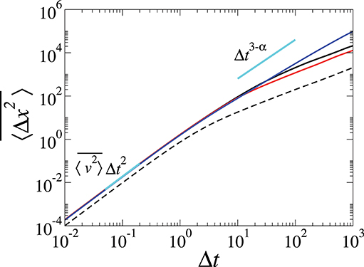
Figure 4. Time-averaged MSDs. The three solid curves correspond to the case of P(τ), respectively, the poissonian (black), gaussian (red), and the power-law (blue). For reference, the underdamped Brownian particle with f(t) = 0 is plotted together (dashed). Additionally, the theoretical expectation (thick cyan) of $\overline{\langle v^2\rangle }\Delta t^2$, Equation 18, is overlaid with the simulation data. The simulations were carried out based on the equation of motion 1 with v₀ = 0, timestep δt = 0.01, and with 10⁵ random realizations of f(t). The same parameter values used in Figure 3. The basic units are: $\left[x\right]=1/\sqrt{\beta \sigma }$, $\left[t\right]=\sqrt{m/(\beta \sigma )}$.

Additionally, we simulate the overdamped Langevin equation 27 and obtain, in Figure 5, the fully averaged MSDs for the three cases of f. In the plot, the gray dots show sample time-averaged MSDs from individual trajectories and their average curve over 10⁶ ensemble is depicted with solid red line. This MSD is overlaid with our theoretical expression (Equation 35) explaining the full-time (overdamped) dynamics with information of P(τ). It confirms that our analytic theory correctly explains the overdamped dynamics in the full range of time. Here, the MSD initially grows as 2DΔt (plotted as cyan). Then the MSD has a cross-over at Δt ~ [τ]_T and beyond it reaches the large-time limit. For the poissonian and gaussian PDFs the large-time motion is Fickian with the increased diffusivity D_L. Consistently with Figure 4, for the overdamped Langevin model of Equation (27) a superdiffusion of Δt^3−α is observed for the power-law PDF.

FIGURE 5

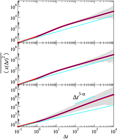
Figure 5. Time-averaged MSDs for the overdamped Langevin dynamics from Equation 27. From Top to Bottom the cases for the poissonian, gaussian, and the power-law PDFs of P(τ), respectively. Gray dots show the time-averaged MSD curves from single trajectories generated from simulation and the solid (red) line represents their average over 10⁶ realizations. Blue lines are the theoretical curves of Equation 35. The Langevin simulation was carried out with timestep δt = 0.01, D = 1, and T = 10⁵. For the f(t) the same PDFs of ${P}(f)$ and P(τ) informed in Figures 3, 4 were used. The units in our overdamped Langevin simulation (Equation 27) are: $\left[x\right]=D/\sqrt{\tilde{\sigma }}$, $\left[t\right]=D/\tilde{\sigma }$.

3.3. Displacement PDFs and Gaussianity

In Figure 6 (Bottom) we present the displacement PDFs, p(x, t), for the active dynamics shown in our overdamped Langevin model Equation 27. The PDFs are obtained for the three distinct P(τ)s and for three MSD regimes (Left: short-time, Middle: cross-over, Right: long-time). Top panel in Figure 6 shows the evolution of the non-gaussian parameter E[x⁴(t)]/(3E[x²(t)]²) (where E[x^m(t)] ≡ ∫dxx^mp(x, t)) [1], which is zero for a gaussian process. Comparing with the MSD in Figure 5, we see that the displacement PDF has the unique feature in each regime: Namely, when the particle dynamics is Fickian with D, the displacement PDF is gaussian. Entering the cross-over regime, the MSD has a transient superdiffusion where the p(x, t) most deviates from the gaussianity. In the long-time regime, interestingly, the p(x, t) recovers the gaussian property for the poissonian and gaussian P(τ)s which exhibits the Fickian dynamics with D_L, although the particle is constantly under a nonequilibrium state due to f(t). For the power-law P(τ) (α = 1.2), leading to the long-time superdiffusion in MSD, the displacement is severely deviated from gaussianity because of the violation of the central limit theorem (CLT). Note that our power-law P(τ), different from the former two PDFs, is a heavy-tailed PDF having the diverging second moment ∫ dττ²P(τ) = ∞. Thus, the variance of typical displacement due to f(t) over one event, $\tilde{\lambda }(t,t+\tau )=\frac{f}{\gamma }\tau$, diverges (see Equation 29) and breaks down the CLT. We learn from this result that the P(τ) not only determines the long-time dynamics but also affects the gaussianity.

FIGURE 6

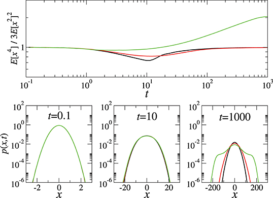
Figure 6. Gaussianity test (Top) and the corresponding displacement PDFs p(x, t) (Bottom) for the overdamped Langevin motion of Equation (27). In the panels, each line represents, respectively, the result for the poissonian (red), gaussian (black), and the power-law (green) PDF of P(τ). Parameters in P(τ) were used as in the previous simulation for MSDs. The displacement PDFs were obtained from 10⁸ simulation runs with T = 10⁴, δt = 0.001, and $D=\tilde{\sigma }=1$. The basic units are: $\left[x\right]=D/\sqrt{\tilde{\sigma }}$, $\left[t\right]=D/\tilde{\sigma }$.

We investigate the effect of ${P}(f)$ on the gaussianity. For this purpose, we simulate the cases where ${P}(f)$s are two-stated and gaussian under the three P(τ)s considered. Figure 7 presents the evolution of the non-gaussian parameter for the corresponding Langevin dynamics. From Top to Bottom, the panels show the results for the poissonian, gaussian, and the power-law P(τ), respectively. In each panel, the three curves indicate those from a uniform (red), a two-state (green), and a gaussian (black) ${P}(f)$. The figure shows two interesting observations. The Langevin dynamics (Equation 27) is always gaussian for all times, irrespective of P(τ), if ${P}(f)$ is gaussian; otherwise, it exhibits qualitatively the same feature shown in Figure 6, where the long-time motion eventually attains gaussianity for the poissonian and gaussian P(τ) while it is non-gaussian for the heavy-tailed P(τ). Previously, similar studies on the gaussianity for the processes described by a generalized Langevin equation were reported in Oliveira et al. [29] and Lapas et al. [36].

FIGURE 7

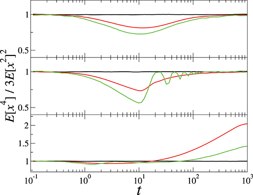
Figure 7. The effect of ${P}(f)$ on the gaussianity of the overdamped Langevin dynamics Equation (27). Three models of ${P}(f)$ are the uniform distribution ${P}(f)=1/(2\sqrt{3})$ in $\left[-\sqrt{3},\sqrt{3}\right]$ (red), the gaussian ${P}(f)=exp(-f^2/2)/\sqrt{2\pi }$ (black), and the two-state ${P}(f)=\frac{1}{2}\delta (f+1)+\frac{1}{2}\delta (f-1)$ (green). From Top to Bottom, the panels show the non-gaussian parameters for the three models under the P(τ): poissonian (Top), gaussian (Middle), and the power-law (Bottom). The simulation parameters are same as in Figure 6.

4. Discussion and Conclusions

In this work, we investigated the dynamics of a Brownian particle in the presence of a telegraphic random force f(t), which acts as a nonequilibrium noise from the environment and mimics the active force experienced in an active bath. We presented an analytic method to solve the Langevin equation 1 for a given telegraphic time series of f(t) and theoretically studied the active dynamics of the particle in terms of the velocity autocorrelation, heat rate, and the MSD. Analytic expressions of these observables were derived within a proper approximation for three distinct types of f(t) having a poissonian, gaussian, and a power-law PDFs of the noise duration time P(τ). To complement this analytic study, we simulated the corresponding Langevin active systems and computationally investigated the same physical observables that fully averaged over the noise amplitude and duration time. It was validated that the numerically observed dynamic behaviors are quantitatively well explained by the analytic results.

It turns out that in the presence of the telegraphic f(t) the heat rate is nonzero for all times, which implies the imbalance between thermal fluctuation and dissipation due to the f(t). The effect of the active noise is present not only in the FDT violation but also in the long-time apparent diffusivity D_L. It was shown that $D_L>D(={\beta }^{-1}/\gamma )$ (see Equation 37) where the difference D_L−D is proportional to the strength of f(t) as shown in $\langle \stackrel{\cdot }{Q}\rangle$, as long as the variance of duration time is finite: If this diverges, D_L diverges as well and the transport becomes anomalous (superdiffusive).

4.1. Active Particle Under Confinement

We emphasize that our current model essentially describes the transport dynamics of an active particle under confinement. Consider the overdamped Langevin dynamics of a particle under a confining harmonic potential in the presence of the active telegraphic force f(t). The equation of motion reads

$\begin{array}{ll}\gamma \dot{x}=-\kappa x+\xi (t)+f(t),& (40)\end{array}$

where κ is the stiffness constant of the harmonic potential such as the optical trap. By replacing v → x, γ → κ/γ, σ → σ/γ², and β → κβ, our original Langevin equation 1 is mapped to Equation 40. Therefore, by analogy, all the analytic results presented in our work can be applied to this problem. For instance, the autocorrelation of x(t) can be directly read off from Equations 14 and 19. It is inferred that the MSD grows linearly as $\overline{\langle \Delta x^2\rangle }~\Delta t$ at the beginning, approaching to

$\begin{array}{ll}\overline{\langle \Delta x^2\rangle }\approx 2{(\beta \kappa )}^{-1}+2\frac{\sigma }{{\kappa }^2}\left(1-\frac{1-e^{-\kappa {\left[\tau \right]}_T/\gamma }}{\kappa {\left[\tau \right]}_T/\gamma }\right)& (41)\end{array}$

as Δt → ∞.

4.2. The Run-and-Tumble Dynamics

The locomotion dynamics of bacterial micro-swimmers has been investigated with great interest in the viewpoint of a self-propelled particle [2, 19, 33, 37–40]. Our Langevin model and the presented study of the model provide an insight into the so-called run-and-tumble dynamics of bacteria. In our model, the run and tumble states can be represented by a telegraphic noise f(t) having the zero state of f_i = 0. The simplest case is the three-state model allowing only the discrete amplitudes f_i = −f₀, 0, +f₀. A continuous model expanding the three-state model can be ${P}(f)=q\delta (f)+(1-q){{P}}_r(f)$ with a ratio q (0 < q < 1). ${{P}}_r(f)$ is a normalized bimodal PDF for the run states. With a proper ${P}(f)$ and P(τ), the experimentally observed run-and-tumble dynamics can be quantitatively explained. Typically, the run-and-tumble dynamics is modeled with a time-independent constant transition rate between the two phases [41, 42]. In our model, this is the case governed by the poissonian P(τ). It is inferred from our study that this type of run-and-tumble dynamics eventually reaches the Fickian regime, as consistent with previous experimental and theoretical studies [42–44]. We also anticipate that even if the transition rate is weakly time-dependent (i.e., the gaussian P(τ) in our model) the long-time Fickian dynamics is still present. Namely, for any P(τ) having a well-defined cutoff timescale, the Fickian dynamics is universal. Another interesting feature is that before this Fickian nonequilibrium state is reached a superdiffusive dynamics can be transiently observed, as seen in Figure 5. For the power-law PDFs of the run and tumble times, their long-time dynamics may vary from the ballistic over a sub-ballistic superdiffusion to the Fickian depending on the power-law exponent α. A superdiffusive dynamics of swarming B. subtilis, $\overline{\langle \Delta x^2\rangle }~\Delta t^{1.6}$, reported in [45] may be an example of this type.

4.3. Connection to Lévy Walks

As commented above and also seen in Equation 39, our Langevin model with a power-law P(τ) are intimately related to the Lévy walk model. Especially, if the active force only has two states (f_i = −f₀, +f₀), our overdamped Langevin model Equation 27 describes a Lévy walk in the presence of thermal noise. Conceptually, this model can be understood as a noisy continuous-time random walks introduced in Song et al. [4] and Jeon et al. [46]. The thermal effect yields the linear growth of MSD (~Δt) at the beginning, otherwise absent, before the ballistic regime appears in the intermediate regime. At large times the thermal noise will be ignored and the well-known Lévy walk dynamics emerge. In Figure 8, we simulate this noisy Lévy walk process in our overdamped Langevin model with the power-law P(τ) of α = 1.2. The simulation procedure is the same as that of our overdamped model with the power-law P(τ) (in Figures 5, 6) but the continuous amplitude PDF is replaced to ${P}(f)=\frac{1}{2}\delta (f+f_0)+\frac{1}{2}\delta (f-f_0)$. Further information on the simulation is provided in the Appendix and the Caption in Figure 8. The simulated Langevin process is consistent with a sub-ballistic Lévy walk with the sojourn time power-law PDF of 1 < α < 2 [9]. The MSD at large times grows as ~Δt^3−α expected in the sub-ballistic Lévy walk [9, 45, 47]. The p(x, t)s exhibit the sharp peaks at the end of the distribution, which originates from the ballistic front of a Lévy walk representing the cases that the first active noise remains survived until the measurement time t [9]. A small difference is the spread of the ballistic front shown in p(x, t) (Figure 8, Right). This broadening is the outcome of thermal noise. The survival probability of the ballistic front ${\text{Ψ}}_s(t)={\int }_t^{\infty }P(\tau )d\tau$ decays as a power-law of t^−α. The average survival time of the first active noise ∫ dttΨ_s(t) is finite for all α > 1. Thus, the peaks eventually decay out with time, as seen in Figure 8 (Right), and the p(x, t) becomes a unimodal distribution. It is worths comparing our noisy Lévy walk with the two-state transition model introduced by Malakar et al. [33]. The latter model can be understood as a variant of our noisy Lévy walk where the power-law P(τ) is replaced to the poissonian PDF. In this case, as shown in section 2.3, the long-time diffusion dynamics becomes Fickian with an apparent diffusivity 37 after the cross-over superdiffusive regime. The p(x, t) of this model can have the sharp peaks (the ballistic front) at the tails in the cross-over regime if the thermal noise is sufficiently weak. The multi-modal distribution eventually returns to a gaussian distribution in the long-time Fickian regime [33]. This is in agreement with the gaussianity behavior of our corresponding model shown in Figure 7 [the two-state ${P}(f)$ & poissonian P(τ)].

FIGURE 8

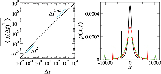
Figure 8. MSD (Left) and p(x, t) (Right) of the overdamped Langevin model Equation 27 for the two-state model of f_i(= ±1). The p(x, t) are plotted at t = 8,000 (black), 9,000 (red), and 10,000 (green). For the duration time, the power-law PDF with α = 1.2 was used. The simulation details were same as in Figure 5. The data were obtained from 10⁵ simulation runs. The basic units are: $\left[x\right]=D/\sqrt{\tilde{\sigma }}$, $\left[t\right]=D/\tilde{\sigma }$.

Finally, we note in passing that for the power-law PDFs our active process will suffer the aging dynamics. This aging effect will be investigated in depth as further work.

Data Availability Statement

The appendix of this paper is included in the manuscript/Supplementary Files.

Author Contributions

JU, TS, and J-HJ designed the model, performed the analytic and computational invetigations, and wrote the paper together.

Funding

This work was supported by the National Research Foundation (NRF) of Korea through No. 2017R1D1A1B03030872 (JU), No. 2017R1D1A1B03034600 (TS), and No. 2017R1C1B2007555 (J-HJ).

Conflict of Interest

The authors declare that the research was conducted in the absence of any commercial or financial relationships that could be construed as a potential conflict of interest.

Supplementary Material

The Supplementary Material for this article can be found online at: https://www.frontiersin.org/articles/10.3389/fphy.2019.00143/full#supplementary-material

References

1. Metzler R, Jeon JH, Cherstvy AG, Barkai E. Anomalous diffusion models and their properties: non-stationarity, non-ergodicity, and ageing at the centenary of single particle tracking. Phys Chem Chem Phys. (2014) 16:24128–64. doi: 10.1039/C4CP03465A

PubMed Abstract | CrossRef Full Text | Google Scholar

2. Bechinger C, Di Leonardo R, Löwen H, Reichhardt C, Volpe G, Volpe G. Active particles in complex and crowded environments. Rev Mod Phys. (2016) 88:045006. doi: 10.1103/RevModPhys.88.045006

CrossRef Full Text | Google Scholar

3. Riedel C, Gabizon R, Wilson CAM, Hamadani K, Tsekouras K, Marqusee S, et al. The heat released during catalytic turnover enhances the diffusion of an enzyme. Nature. (2014) 517:227–30. doi: 10.1038/nature14043

PubMed Abstract | CrossRef Full Text | Google Scholar

4. Song MS, Moon HC, Jeon JH, Park HY. Neuronal messenger ribonucleoprotein transport follows an aging Lévy walk. Nat Commun. (2018) 9:344. doi: 10.1038/s41467-017-02700-z

PubMed Abstract | CrossRef Full Text | Google Scholar

5. Wu XL, Libchaber A. Particle Diffusion in a Quasi-Two-Dimensional Bacterial Bath. Phys Rev Lett. (2000) 84:3017–20. doi: 10.1103/PhysRevLett.84.3017

PubMed Abstract | CrossRef Full Text | Google Scholar

6. Fodor E, Hayakawa H, Tailleur J, van Wijland F. Non-Gaussian noise without memory in active matter. Phys Rev E. (2018) 98:062610. doi: 10.1103/PhysRevE.98.062610

CrossRef Full Text | Google Scholar

7. Chen DTN, Lau AWC, Hough LA, Islam MF, Goulian M, Lubensky TC, et al. Fluctuations and rheology in active bacterial suspensions. Phys Rev Lett. (2007) 99:148302. doi: 10.1103/PhysRevLett.99.148302

PubMed Abstract | CrossRef Full Text | Google Scholar

8. Dev S, Chatterjee S. Run-and-tumble motion with steplike responses to a stochastic input. Phys Rev E. (2019) 99:012402. doi: 10.1103/PhysRevE.99.012402

PubMed Abstract | CrossRef Full Text | Google Scholar

9. Zaburdaev V, Denisov S, Klafter J. Lévy walks. Rev Mod Phys. (2015) 87:483–530. doi: 10.1103/RevModPhys.87.483

CrossRef Full Text | Google Scholar

10. Gal N, Weihs D. Experimental evidence of strong anomalous diffusion in living cells. Phys Rev E. (2010) 81:020903. doi: 10.1103/PhysRevE.81.020903

PubMed Abstract | CrossRef Full Text | Google Scholar

11. Chen K, Wang B, Granick S. Memoryless self-reinforcing directionality in endosomal active transport within living cells. Nat Mater. (2015) 14:589–93. doi: 10.1038/nmat4239

PubMed Abstract | CrossRef Full Text | Google Scholar

12. Berg HC, Borowski A, De Vivie ER. E. coli in Motion. In: Biological and Medical Physics, Biomedical Engineering. Springer (2004).

Google Scholar

13. Ramos-Fernandez G, Mateos J, Miramontes O, Germinal C, Larralde H, Ayala-Orozco B. Lévy walk patterns in the foraging movements of spider monkeys (Ateles geoffroyi). Behav Ecol Sociobiol. (2003) 55:223–30. doi: 10.1007/s00265-003-0700-6

CrossRef Full Text | Google Scholar

14. Sagi Y, Brook M, Almog I, Davidson N. Observation of anomalous diffusion and fractional self-similarity in one dimension. Phys Rev Lett. (2012) 108:093002. doi: 10.1103/PhysRevLett.108.093002

PubMed Abstract | CrossRef Full Text | Google Scholar

15. Brockmann D, Hufnagel L, Geisel T. The scaling laws of human travel. Nature. (2006) 439:462–5. doi: 10.1038/nature04292

PubMed Abstract | CrossRef Full Text | Google Scholar

16. Reynolds AM, Rhodes CJ. The Lévy flight paradigm: random search patterns and mechanisms. Ecology. (2009) 90:877–87. doi: 10.1890/08-0153.1

PubMed Abstract | CrossRef Full Text | Google Scholar

17. Chaki S, Chakrabarti R. Enhanced diffusion, swelling, and slow reconfiguration of a single chain in non-Gaussian active bath. J Chem Phys. (2019) 150:094902. doi: 10.1063/1.5086152

PubMed Abstract | CrossRef Full Text | Google Scholar

18. Mandelbrot B, Van Ness J. Fractional brownian motions, fractional noises and applications. SIAM Rev. (1968) 10:422–37. doi: 10.1137/1010093

CrossRef Full Text | Google Scholar

19. Barthelemy P, Bertolotti J, Wiersma DS. A Lévy flight for light. Nature. (2008) 453:495–8. doi: 10.1038/nature06948

PubMed Abstract | CrossRef Full Text | Google Scholar

20. Jeon JH, Monne HMS, Javanainen M, Metzler R. Anomalous diffusion of phospholipids and cholesterols in a lipid bilayer and its origins. Phys Rev Lett. (2012) 109:188103. doi: 10.1103/PhysRevLett.109.188103

PubMed Abstract | CrossRef Full Text | Google Scholar

21. Ernst D, Hellmann M, Köhler J, Weiss M. Fractional Brownian motion in crowded fluids. Soft Matt. (2012) 8:4886–9. doi: 10.1039/c2sm25220a

CrossRef Full Text | Google Scholar

22. Weiss M. Single-particle tracking data reveal anticorrelated fractional Brownian motion in crowded fluids. Phys Rev E. (2013) 88:010101. doi: 10.1103/PhysRevE.88.010101

PubMed Abstract | CrossRef Full Text | Google Scholar

23. Weber SC, Spakowitz AJ, Theriot JA. Bacterial chromosomal loci move subdiffusively through a viscoelastic cytoplasm. Phys Rev Lett. (2010) 104:238102. doi: 10.1103/PhysRevLett.104.238102

PubMed Abstract | CrossRef Full Text | Google Scholar

24. Jespersen S, Metzler R, Fogedby HC. Lévy flights in external force fields: langevin and fractional Fokker-Planck equations and their solutions. Phys Rev E. (1999) 59:2736. doi: 10.1103/PhysRevE.59.2736

CrossRef Full Text | Google Scholar

25. Lisowski B, Valenti D, Spagnolo B, Bier M, Gudowska-Nowak E. Stepping molecular motor amid Lévy white noise. Phys Rev E. (2015) 91:042713. doi: 10.1103/PhysRevE.91.042713

PubMed Abstract | CrossRef Full Text | Google Scholar

26. Van Den Broeck C. On the relation between white shot noise, Gaussian white noise, and the dichotomic Markov process. J Stat Phys. (1983) 31:467–83. doi: 10.1007/BF01019494

CrossRef Full Text | Google Scholar

27. Luczka J. Non-Markovian stochastic processes: colored noise. Chaos. (2005) 15:026107. doi: 10.1063/1.1860471

PubMed Abstract | CrossRef Full Text | Google Scholar

28. Barik D, Ghosh PK, Ray DS. Langevin dynamics with dichotomous noise: direct simulation and applications. J Stat Mech. (2006) 2006:P03010. doi: 10.1088/1742-5468/2006/03/P03010

CrossRef Full Text | Google Scholar

29. Oliveira FA, Ferreira RMS, Lapas LC, Vainstein MH. Anomalous diffusion: a basic mechanism for the evolution of inhomogeneous systems. Front Phys. (2019) 7:18. doi: 10.3389/fphy.2019.00018

CrossRef Full Text | Google Scholar

30. Onsager L, Machlup S. Fluctuations and irreversible processes. Phys Rev. (1953) 91:1505–12. doi: 10.1103/PhysRev.91.1505

CrossRef Full Text | Google Scholar

31. Kwon C, Um J, Park H. Information thermodynamics for a multi-feedback process with time delay. Europhys Lett. (2017) 117:10011. doi: 10.1209/0295-5075/117/10011

CrossRef Full Text | Google Scholar

32. Sekimoto K. Langevin equation and thermodynamics. Prog Theor Phys Suppl. (1998) 130:17–27. doi: 10.1143/PTPS.130.17

CrossRef Full Text | Google Scholar

33. Malakar K, Jemseena V, Kundu A, Kumar V, Sabhapandit S, Majumdar SN, et al. Steady state, relaxation and first-passage properties of a run-and-tumble particle in one-dimension. J Stat Mech. (2018) 043215. doi: 10.1088/1742-5468/aab84f

CrossRef Full Text | Google Scholar

34. Hayot F. Lévy walk in lattice-gas hydrodynamics. Phys Rev A. (1991) 43:806–10. doi: 10.1103/PhysRevA.43.806

PubMed Abstract | CrossRef Full Text | Google Scholar

35. Solomon TH, Weeks ER, Swinney HL. Observation of anomalous diffusion and Lévy flights in a two-dimensional rotating flow. Phys Rev Lett. (1993) 71:3975–8. doi: 10.1103/PhysRevLett.71.3975

PubMed Abstract | CrossRef Full Text | Google Scholar

36. Lapas LC, Costa IVL, Vainstein MH, Oliveira FA. Entropy, non-ergodicity and non-Gaussian behaviour in ballistic transport. Europhys Lett. (2007) 77:37004. doi: 10.1209/0295-5075/77/37004

CrossRef Full Text | Google Scholar

37. Cates ME, Tailleur J. Motility-induced phase separation. Annu Rev Condens Matt Phys. (2015) 6:219–44. doi: 10.1146/annurev-conmatphys-031214-014710

CrossRef Full Text | Google Scholar

38. Darnton NC, Turner L, Rojevsky S, Berg HC. Dynamics of bacterial swarming. Biophys J. (2010) 98:2082–90. doi: 10.1016/j.bpj.2010.01.053

PubMed Abstract | CrossRef Full Text | Google Scholar

39. Di Leonardo R, Angelani L, Dell'Arciprete D, Ruocco G, Iebba V, Schippa S, et al. Bacterial ratchet motors. Proc Natl Acad Sci USA. (2010) 107:9541–5. doi: 10.1073/pnas.0910426107

PubMed Abstract | CrossRef Full Text | Google Scholar

40. Saragosti J, Calvez V, Bournaveas N, Perthame B, Buguin A, Silberzan P. Directional persistence of chemotactic bacteria in a traveling concentration wave. Proc Natl Acad Sci USA. (2011) 108:16235–40. doi: 10.1073/pnas.1101996108

PubMed Abstract | CrossRef Full Text | Google Scholar

41. Najafi J, Shaebani MR, John T, Altegoer F, Bange G, Wagner C. Flagellar number governs bacterial spreading and transport efficiency. Sci Adv. (2018) 4:eaar6425. doi: 10.1126/sciadv.aar6425

PubMed Abstract | CrossRef Full Text | Google Scholar

42. Lee M, Szuttor K, Holm C. A computational model for bacterial run-and-tumble motion. J Chem Phys. (2019) 150:174111. doi: 10.1063/1.5085836

CrossRef Full Text | Google Scholar

43. Thiel F, Schimansky-Geier L, Sokolov IM. Anomalous diffusion in run-and-tumble motion. Phys Rev E. (2012) 86:021117. doi: 10.1103/PhysRevE.86.021117

PubMed Abstract | CrossRef Full Text | Google Scholar

44. Fier G, Hansmann D, Buceta RC. Langevin equations for the run-and-tumble of swimming bacteria. Soft Matt. (2018) 14:3945–54. doi: 10.1039/C8SM00252E

PubMed Abstract | CrossRef Full Text | Google Scholar

45. Ariel G, Rabani A, Benisty S, Partridge JD, Harshey RM, Be'er A. Swarming bacteria migrate by Lévy Walk. Nat Commun. (2015) 6:8396. doi: 10.1038/ncomms9396

PubMed Abstract | CrossRef Full Text | Google Scholar

46. Jeon JH, Barkai E, Metzler R. Noisy continuous time random walks. J Chem Phys. (2013) 139:121916. doi: 10.1063/1.4816635

PubMed Abstract | CrossRef Full Text | Google Scholar

47. Froemberg D, Barkai E. Time-averaged Einstein relation and fluctuating diffusivities for the Lévy walk. Phys Rev E. (2013) 87:030104. doi: 10.1103/PhysRevE.87.030104

CrossRef Full Text | Google Scholar