From Micro-to-Macro: How the Movement Statistics of Individual Walkers Affect the Formation of Segregated Territories in the Territorial Random Walk Model

Animal territoriality is a widespread phenomena in many vertebrate species. In mammals it is often associated with territorial marking with which individuals make their presence conspicuous to others by leaving trace of their passage, often in the form of deposited scent. A simple interaction mechanism consisting of retreating upon the encounter of a foreign scent is sufficient to observe the emergence of territorial patterns at the population level. With the introduction of the so-called territorial random walk model this local avoidance mechanism coupled with a simple diffusive movement of the individuals has been shown to generate long-lasting patterns of segregation at much larger spatial scales. To shed further light on the micro-to-macro connection of this collective movement model we study how the movement statistics of the individuals affect the formation of the segregated scented territories. We represent individual animals as correlated random walkers and we analyse the spatial ordering of the population as a function of the length of time a scent mark remains active after deposition and as a function of the degree of correlation of the movement steps. For low and intermediate correlation strength we find that territories undergo a liquid-hexatic-solid transition as active scent time is increased. Increased spatial order also appears by increasing the correlation strength but only if well away from the ballistic limit. We ascribe this non-monotonic dependence to the coverage efficiency of the individual walkers mainly controlled by the correlation and the mobility of the territories mainly controlled by the active scent time.

1. Introduction and Background

In biology it is rather common to find a system in which the underlying movement of its constituent parts is not diffusive, often owed to the out-of-equilibrium nature of the processes involved. Examples of anomalous transport can be found at all scales: from the active and passive microrheology of various nanoparticles inside the molecularly crowded environment of cells [1] and the two stage diffusion of macromolecules on cell membranes [2, 3] to the superdiffusive displacement of epithelial cells [4], and all the way to the anomalous dynamics of whole organism while foraging randomly [5] or during memory biased search [6, 7].

Among the cited biological examples characterized by anomalous diffusion we have focused for this special issue on the movement of whole organisms and on the collective effects of many such organisms spatially excluding one another. Our interest here lies in understanding how the local statistical features of the movement of individual animals affect the emergence of the collective patterns at the population level. We choose a movement statistics that becomes random at long time scales, but retains a degree of persistence at shorter time scales, the so-called correlated random walker [8], a paradigmatic movement model in animal ecology [9, 10]. Among the forms of spatial exclusion or avoidance we are particularly interested in a very common behavior of vertebrate populations in 2D: the subdivision of the terrain into spatially segregated regions [11]. When these regions are of exclusive ownership of a single individual or a single family unit they are called territories [12, 13].

The purposes of territoriality change from species to species or even throughout the year [14]. These include, roosting, mating, nesting, and harboring resources. Accordingly the interaction mechanisms that animals rely upon to form and maintain these territories are quite rich and depend on the type of signals that animals exchange. Broadly speaking one may distinguish them between direct and indirect, that is whether the time scale for the signals to travel from the emitter to the receiver is short or long relative to the time scale for the emitter to move. Examples of direct interactions, often employed by birds [15], is the use of visual displays and audio calls. In this case the signal of the emitter is detected by the receiver nearly instantaneously. Examples of indirect interaction, used by a large number of mammals [16], is the use of olfactory cues. In this case the scent that an animal deposits is nearly static. For the period over which the scent remains detectable, which could be a long time after deposition, the environment retains the memory of the passage of the emitter. Any individual that comes in close proximity to the deposited scent becomes a receiver and acquires information about the (past) presence of the emitter.

In this study we analyse a specific case of olfactory-based territorial formation, often called conspecific avoidance, whereby animals mark the terrain wherever they go, and other individuals passing by respond to these olfactory cues by retreating from the region or area where foreign scent was encountered. This indirect animal interaction, that occurs through the modification of the environment, is called stigmergy [17]. It is a common form of interaction in eusocial insects [18], but it has been shown to occur also in territorial animals [19].

The mathematical study of scent-marked territorial patterns has a relatively long history dating back to the early '90s when the first reaction-diffusion model representing a pair of animals avoiding each other scent was formulated [20]. This model coupled the occupation probability of two Brownian walkers tethered to their respective den or burrow and their scent profiles. It was later generalized to include the effects of landscape heterogeneity and animal movement responses and applied to movement data on wolves and coyotes [21].

In subsequent modeling studies on the formation of scented territories a different approach was followed [22]. That approach becomes necessary when one aims to account for the sharp spatial dependence of the interaction. In these cases the field nature of the interaction potentials (or forces), which tacitly assumes that they are defined at every point in space, may not be adequate. It is more convenient to account for the interaction dynamics through localized walls or spatial partitions representing the deposited scent [23]. By doing so one remains faithful to the biology of scent-marking species for which individuals react to the encounter of foreign scent only if it is informative, that is only if the deposition occurred before a certain time in the past [see e.g., Alberts [24]].

As this approach requires tracking the movement and interaction of the entire population to determine the time-dependent position of each animal and the age of the scent deposited, it was formulated as an individual based model [22]. This increased complexity, however, allows to consider animals that do not have a den or a burrow as well as to study the emergence of territorial patterns as a collective phenomena rather than a two-body problem between neighboring individuals.

The collective movement model of territory formation, termed the territorial random walk (TRW) model [23], lends itself naturally to questions on the nature of the emerging patterns, e.g., if macroscopic order and/or disorder phases appear and how the microscopy of the movement and interaction rules influence the emergence of the macroscopic patterns. Along these lines a very recent investigation on the presence of order-disorder phase transitions in the TRW model as a function of the scent decay time and the population density has been conducted [25]. In that study it has been shown that the emerging territorial patterns display a solid to liquid melting scenario analogous to the one supported by the Kosterlitz-Thouless-Halperin-Nelson-Young (KTHNY) theory of melting [26–28], with the appearance of an intermediate partially ordered phase, called hexatic, due to the importance of geometrical arrangements of the first six neighbors.

Here we extend that analysis by considering a more realistic movement model for the individual animals. We modify the movement statistics of the animal by representing them as correlated random walkers and we ask how the “microscopic” movement of the individuals alters the collective dynamics of the system and the order-disorder scenario.

The paper is organized as follows. In section 2 we introduce the model and we present details of the stochastic simulations and the thermalization of the system. The analysis has two parts to it. At the “microscopic” level, that is at the level of the individuals, we study the influence of the persistence of the walk on the variance of the occupation probability, that is the mean square displacement (MSD). This is presented in section 3 together with an analysis of the spatial coverage of each walker in its own territory. As we scale up to the level of the territories, we analyse the effects of the animal movement statistics on the appearance of ordered phases in the system. This is dealt with in section 4. And finally section 5 presents concluding remarks.

2. The Correlated Territorial Random Walker Model

The correlated territorial random walker (cTRW) model, an extension of the TRW model, is a lattice-based collective movement model where individuals move with some degree of persistence, that is the movement direction at each time step depends on the previous step direction. The model can be run in any dimension and in discrete or continuous time. For computational efficiency we have run it in discrete time and we have only analyzed the 2D case. To study the structure of the emerging territories it is important not to introduce spatial frustration effects and we have thus used a triangular lattice with periodic boundary conditions.

In the absence of interactions a walker's steps are correlated. To model the persistent random walk on a triangular lattice we start from a continuous turning angle variable θ ∈ (−π, π], and we create six bins of width $\frac{\pi }{3}$ for each of the turns a walker can make. The angle θ is then drawn randomly from a wrapped Cauchy distribution, ${C}(\theta )=(1-{\rho }^2){\left[2\pi (1+{\rho }^2-2\rho cos(\theta ))\right]}^{-1}$ where −π ≤ θ < π and ρ is the persistence parameter, or the mean cosine of the distribution. It indicates the tendency of a walker to continue to move in the same direction from where it came from at the previous step. In the limit ρ → 0, the distribution reduces to ${C}(\theta )=\frac{1}{2\pi }$ i.e., the turning angles are uniformly distributed and the movement of the walker becomes random. The opposite limit corresponds to the ballistic case ${C}(\theta )\to \delta (\theta )$, where δ(θ) is the Dirac delta function as ρ → 1.

Avoidance between individuals occurs as follows. As animals deposit marks wherever they go, at each time step any individual may encounter one of its own marks or may step on a lattice site with one or multiple foreign marks. When an animal encounters its own marks, no interaction occurs. On the other hand upon encountering a foreign mark within a time period shorter or equal to the so called active scent time T_A from when it was deposited, an interaction occurs. In order to avoid intruding further into neighboring territories. An interaction consists of one of three types of retreat at the following time step. These are in order of preference, first toward a neighboring site with no scent marks, second toward a neighboring site with the animal's own scent and lastly in the rare case where neither of the previous options are available the animal moves randomly to one of the six neighboring sites. At the subsequent step the animal reorients itself with a new direction chosen at random between the six potential choices.

As a result of the above interactions, foreign scents serve as spatial barriers effectively making individuals avoid entering further into others' territories. At any given time t a territory is represented by all the sites that contain an active scent of a specific animal. Alternatively it represents the sites an individual has visited within the interval (t − T_A, t). Except at the boundaries, where a given territory may overlap with one or more neighboring ones, the avoidance of region recently visited by other individuals create spatially segregated areas of exclusive ownership for each animal.

The spatio-temporal dynamics of the territories can be fast and slow depending on the choice of parameters, which are, respectively, the inverse of the population density or specific volume ν = L²/N where L² is the domain size, the active scent time T_A and the persistence parameter ρ. With small T_A and large ν one observes highly mobile and morphing territories as exclusion interactions are not very frequent. The opposite happens with large T_A and small ν as interactions occur more frequently.

The dependence on the initial condition of the system is dealt with by running simulations and waiting for the system to thermalize before making any spatial and/or temporal measurement on appropriate quantities of the system. The thermalization is performed as follows. Two different initial conditions are used. The first is initialized with the scent profile tessellating the available space, i.e., the territory of each walker is a perfect hexagon with all boundary lattice sites overlapping with the neighboring territories. The second is initialized with randomly distributed walkers with no scent profile. The two are left to run until the standard deviation of the territory size across the entire population converges to the same value in the two cases. When that happens the system is deemed to be thermalized.

Rather than exploring the dynamics for different population density we have selected an intermediate value of ν, namely ν = 48 for multiple reasons. On one hand the rich (slow and fast) dynamics can be attained within a limited range of T_A values so that disordered and ordered phases of the system could be observed and studied as a function of ρ. For smaller population densities, as interactions become more infrequent, it becomes harder to observe spatial ordering and we have thus not explored the regime with larger ν. On the other hand smaller values of ν makes the computation very expensive and makes it harder to reach thermalization except for very small values of T_A.

The specific range and resolution of the parameter space ρ − T_A with ν = 48 has been as follows. The active scent time T_A has been chosen in the range between 89 and 1,424 with a resolution of 89, except for specific cases detailed in the figure captions. For the correlation parameter ρ we have used the values 0, 0.15, 0.35, 0.55, 0.75, and 0.95. To ensure that the territories, with the appropriate choice of T_A, can tessellate with equal hexagons the 2D domain, the linear domain size (with periodic boundary conditions) is set to L = 1200 with N = 3 × 10⁴, which corresponds to ν = 48, although we have also used smaller domains e.g., in section 3.

3. Partial “Caging” and Spatial Coverage of the Individual Walkers

The spatial exclusion of the scented territories is a complex collective phenomenon whereby an animal remains confined in certain region of space depending on when and where foreign marks as well as its own marks have been deposited. But this confinement is only partial since a mark has a lifetime and disappears unless an animal remarks that same location within T_A steps. Animals may thus be trapped for some time before escaping. It is possible to observe such partial “caging” by plotting the MSD as a function of time. We do so in Figure 1 where we draw the normalized MSD for T_A = 712, 1,068, and 1,424 for various values of ρ by averaging over all individuals in one simulation (after the system has thermalized). The MSD plots for T_A = 1 and T_A = 89 are additionally shown in Figure A1. We term these snapshot averages to distinguish them from ensemble averages when multiple copies of the system are run.

FIGURE 1

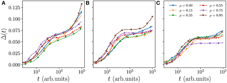
Figure 1. MSD Δ(t) of a walker in a system with ν = 48 and L = 120, where each curve is a snapshot average. The active scent times (T_A) for panels (A–C) are 712, 1,068, and 1,424, respectively. At short timescale the walkers tend to exhibit superdiffusion indicated by the Δ(t)∝t^α relationship where α > 1. For intermediate timescales the dynamics of the walkers are governed by the mobility of their territories. High values of T_A yield slowly moving territories and increase in caging caused by neighbors. This caging saturation is highly sensitive to the correlation of the walkers (see Figure A2) while the time spent at the caging saturation before increasing again is related to the coverage efficiency of the walker.

In moving from panel (a) to (b) and (c) in the figure, that is by increasing T_A, one clearly observes a reduced growth of the curves at intermediate times for each value of ρ. Since a long-time saturating MSD is expected whenever a walker roams inside a finite domain [29], the flattening of the MSD at intermediate times is a manifestation of increased caging from the neighbors. As marks remain active for longer they make the territories progressively less mobile and the MSD curves start increasing again at later times.

A comparison of different values of ρ within the same panel shows that this caging effect becomes stronger—curves remain flat for longer time—for larger ρ except when one approaches the ballistic regime. This is clearly visible in panel (c) when T_A = 1, 424 where this non-monotonicity as a function of ρ can be seen more clearly. There also appears some non-monotonic dependence of the intermediate-time saturation value of the MSD, but this non-monotonicity is only apparent. As we have verified and shown in Figure A2 in the appendix, the intermediate saturation of the MSD is highly erratic as it is very sensitive to the actual shape of the occupation probability for each animal. We consider the time it takes the MSD curve to start increasing again the more significant feature, and to understand the non-monotonicity as a function of ρ we look in detail at the walker spatial coverage.

Considering initially a fixed finite domain, for a walk to improve spatial coverage it needs to reduce spatial oversampling, which clearly happens by increasing ρ. However, in a confined domain, when the degree of correlation is too large, the walker would retrace back its steps thus increasing again the sampling of lattice sites already visited. It is well known in fact that the mean coverage time of an independent walker in a finite domain can be minimized for intermediate values of walk persistence [30, 31].

To test whether this understanding suffices to explain the non-monotonic ρ dependence of the caging effect, we study the walkers' spatial coverage in the cTRW model. As territories are mobile and change shape, we cannot compare values of coverage time for each walker. However, it is possible to obtain information about the efficiency of spatial coverage by plotting the average number of sites an individual covers in a time T_A as a function of ρ. The outcome is shown in Figure 2 where we have plotted C_p, the fraction of sites covered in a time T_A, for different values of ρ and T_A. From the figure it is evident that the partial coverage of the terrain is maximal for intermediate values of ρ and for T_A sufficiently large. As T_A affects the size of the confining domain, the correlation parameter that maximizes coverage depends on how long marks remain on the terrain.

FIGURE 2

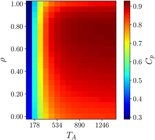
Figure 2. The fraction of the territory defined at time t covered within T_A time steps by walkers as a function of the correlation parameter ρ, and the active scent time T_A. For each pair of ρ and T_A a snapshot average is taken on a thermalized system with L = 120 and ν = 48. For very low T_A the territories are highly volatile, i.e., within a T_A time window the territories are no longer the ones defined at time t which results in low C_p independent of ρ. For higher values of T_A the territories are less mobile and we see the maximization of territory coverage for an intermediate values of ρ.

4. Spatial Ordering of the Emerging Territories

The interaction dynamics of the individual walkers have a long lasting effects on the spatial structure that emerges in the population, as was shown in the case of the simpler TRW model [25]. The spatial ordering of the emerging territories is dictated by the “caging” effect whose size corresponds to the size of the territory. To analyse the spatial ordering as a function of ρ and T_A we look at the system with a coarser temporal and spatial resolution because no order is present at distances smaller than the size of the territory. We neglect the dynamics of the walkers and look at the territory centroids over a T_A time resolution. As territorial centroids are calculated only by considering the mean position of all lattice sites with active scent every T_A steps, we obtain a coarse-grained (continuous-space) mesoscopic time-dependent description of the cTRW model.

4.1. The Pair Correlation Function

For a coarse measure of spatial ordering, we plot in Figure 3 the pair correlation function [32], $g(r)=\nu \langle \sum _{i\ne 0}\delta (|\overrightarrow{r}-\overrightarrow{r_i}|)\rangle$, where δ(z) is the Dirac delta function, as a function of the centroid distance $r=\left|\overrightarrow{r}\right|$ for different ρ and T_A values. In particle systems the pair correlation function gives the likelihood of finding a neighboring particle as a function of distance relative to the ideal gas case. In an ideal gas, g(r) equals 1 for any r as individual particles do not interact with each other and are equally likely to be anywhere in space. A value of zero indicates instead the impossibility of having another particle at that distance in space, e.g., for hard-core interaction of particles of radius σ, g(r) remains zero for all distances up to r = 2σ. Except for extremely small values of T_A, the emerging territories in our model have an effective hard core interaction as can be observed for any of the curves in Figure 3. Those curves remain close to zero up to 2σ where $\sigma =a\sqrt{\nu }/2$, with a the lattice spacing, represents the distance between two evenly spaced centroids when hexagonal territories tessellate the entire domain (see explicit calculation for σ in Heiblum Robles and Giuggioli [25]). A rise from zero to the value one with no evident oscillations would be indicative of a gas with purely hard-core particles. On the other hand a rise beyond the value one with subsequent damped oscillations toward one represents the arrangement of other particles into “shells” of neighbors with the decay pointing to the radial distance over which such spatial ordering persists. Two phases may have qualitatively these characteristics: a liquid but also a hexatic phase. While it is not possible to distinguish a liquid from a hexatic phase from a pair correlation plot, it is possible to determine the appearance of a solid phase because the shells of neighbors are not arranged anymore radially. As a solid possesses hexagonally arranged particles, the radial symmetry is not present anymore and the smoothness of peaks and troughs in the pair correlation function is lost.

FIGURE 3

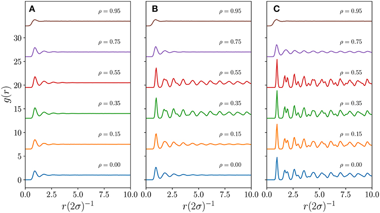
Figure 3. The pair correlation function g(r) for a system with L = 1, 200, ν = 48. Moving from panel (A–C), the T_A values are 712, 1,068, and 1,424, respectively. Within each panel, the g(r) function has been shifted upwards from zero for visualization purposes. For the case ρ = 0 we have used the results from a previous study and as such the T_A values are not precisely the same as the one used for the cases when ρ≠0; they are 707, 1,070, and 1,409 for panels (A–C), respectively. These differences do not take away from the qualitative differences presented here.

A feature that can be evinced by looking at Figure 3 is that the solid phase for sufficiently large T_A appears for intermediate values of persistence ρ. This is particularly evident in panel (b) where the system has radial symmetry at ρ = 0, but then loses it as it approaches ρ = 0.3, and then regains it beyond ρ = 0.55. In panel (c) although the system is already in a solid phase at ρ = 0, the shape of the various g(r) plots also points to a progressive loss, even though only slightly, of radial symmetry as ρ is increased to 0.55, whereas radial symmetry is present when ρ = 0.75. This interesting dependence of the appearance of a solid phase depending both on the value of ρ and T_A matches qualitatively the region in parameter space where the coverage efficiency of an individual is maximized, displayed earlier in Figure 2.

The partial coverage analysis in conjunction with the pair correlation plots indicate that an animal, for a given size of its own territory, that is for a given value of the active scent time T_A, may select the most appropriate correlation statistics to be able to remark the majority of the scented terrain in T_A steps. When that occurs, it implies that the neighbors are kept outside of the terrain that the animal defends. This in turns makes the territories less mobile, reducing the chance of having territory shape far from hexagonal and with large variability in sizes, and the entire population possess a bigger spatial order.

While Figures 2, 3 brings good evidence on how the microscopy of the movement statistics affect the emerging spatial order of the territories for small and intermediate ρ values, it does not seem a viable explanation for large values of ρ. From Figure 2 one would expect in fact a very high order also for ρ = 0.95 and high T_A, but that does not appear to be the case in Figure 3C. However, the system may still possess a great degree of order if it were in an hexatic phase. To determine if that is the case, we first try to use appropriate order parameters that should help us to map out more precisely when the system is in a solid phase as well as to distinguish between a liquid and a hexatic phase as a function of ρ and T_A.

4.2. Order Parameters

In Heiblum Robles and Giuggioli [25] some of the present authors have brought support for a continuous solid-hexatic-liquid transition akin to the KTHNY theory of melting as a function of T_A in the TRW model. Starting from a very high T_A in a perfect crystal configuration, by decreasing T_A below a certain value makes the system loose translational order even though it retains orientational order and no phase coexistence has been observed, the transition being continuous. With a further decrease of T_A the system looses also the orientational order to become liquid. We have extended these results by constructing the orientational and translational order parameters as a function both of ρ and T_A.

We use the so-called local bond-orientational parameter [32] ${\psi }_6(\ell )=\frac{1}{N_{\ell }}\sum _j^{N_{\ell }}exp(i6{\theta }_{\ell ,j})$, where θ_{ℓ, j} is the angle that particle ℓ, located at ${\overrightarrow{r}}_{\ell }$, makes with the j-th neighbor relative to a reference axis, and the j-summation is over the N_ℓ neighbors, the latter obtained through the Voronoi construction [33]. In a perfect crystal, N_ℓ = 6 and ${\theta }_{\ell ,j}=\frac{\pi }{6}$, hence ψ₆(ℓ) = 1. In Figure 4 we visualize qualitatively the changes in orientational order of the system by plotting the argument of the orientational order parameter, arg(ψ₆), for each territory centroid. The orientational ordering of the system, that is when ψ₆ → 1, corresponds to when arg(ψ₆) → 0. From the various subplots one clearly notices that for a given ρ, if one increases T_A, the hexatic phase does not always appear. It is also evident that for T_A < 800 the system cannot reach the hexatic phase independently of the correlation parameter. On the other hand for intermediate values of T_A, e.g., for a given T_A in the range 800–1,100, the system is in a liquid state but then becomes eventually hexatic with sufficiently large ρ, and then liquid again with further increase in ρ. These findings support the pair correlation analysis depicted in Figure 3 and, in addition, they might also give a better idea of whether the system is in an hexatic or a liquid phase, which was not possible by looking only at g(r).

FIGURE 4

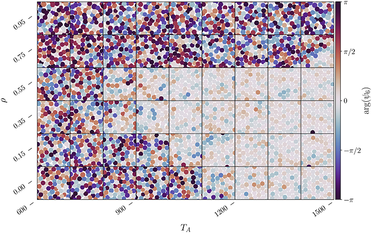
Figure 4. Change in the local bond orientational parameter ψ₆(ℓ) for each territory centroid located at ${\overrightarrow{r}}_{\ell }$ as a function of ρ and T_A. The color of the centroid is determined by arg(ψ₆(ℓ)), while the size of each centroid is proportional to the size of its territory. The system parameters are L = 1, 200 and ν = 48. Each subplot represents subdomain with width L_s = 50, a small fraction of the L² domain, taken at a random location and at some random time after thermalization.

Within the range of where the bond-orientational parameter appears to indicate a hexatic phase, the system may actually be in a solid phase. This can be determined by analyzing the local translational order parameter ${\psi }_t(\ell )=exp(i\overrightarrow{G}·\Delta {\overrightarrow{r}}_{\ell })$, where $\overrightarrow{G}$ is one of the two reciprocal vectors of the simple hexagonal lattice and $\Delta {\overrightarrow{r}}_{\ell }$ is the displacement of the ℓ-th territorial centroid from its ideal lattice site if it were a perfect crystal (ψ_t(ℓ) = 1). The result of such an analysis is shown in Figure 5 where we plot the argument of the local translational order parameter $arg({\psi }_t({\overrightarrow{r}}_{\ell }))$ for each territory. The subplots point to the appearance of a solid phase for intermediate values of ρ and sufficiently large values of T_A, which is when the system is also hexatic when one compares (Figure 4).

FIGURE 5

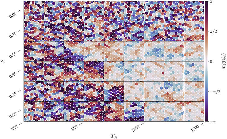
Figure 5. Change in the local translational order parameter ψ_t(ℓ) for each territory centroid located at ${\overrightarrow{r}}_{\ell }$ as a function of ρ and T_A for the system parameters utilized in Figure 4. The color of the centroid is determined by arg(ψ_t(ℓ)), while the size of each centroid is proportional to the size of its territory. Each subplot represents subdomain with width L_s = 50, a small fraction of the L² domain, taken at a random location and at some random time after thermalization.

Given the limited resolution we have employed for the parameters of the system, ρ in particular, it is hard to identify the precise region in parameter space where phase transitions occur. However, by comparing Figures 4, 5 a small hexatic region may exist in a narrow region of parameter space, potentially for 1, 100 ≲ T_A ≲ 1, 300 when ρ = 0.15, for 900 ≲ T_A ≲ 1, 200 when ρ = 0.35, and for 900 ≲ T_A ≲ 1, 200 when ρ = 0.55. This hexatic region should thus be limited on the left by the liquid-hexatic transition and on the right by an hexatic-solid transition.

To try to confirm these qualitative findings we construct the global bond-orientational order parameter ${\text{Ψ}}_6=\left|(1/N)\sum _{\ell }{\psi }_6(\ell )\right|$ and the global translational order parameter ${\text{Ψ}}_t=\left|(1/N)\sum _{\ell }{\psi }_t(\ell )\right|$ and calculate their susceptibility, ${\chi }_6=N\langle {({\psi }_6-\langle {\psi }_6\rangle )}^2\rangle$ and ${\chi }_t=N\langle {({\psi }_t-\langle {\psi }_t\rangle )}^2\rangle$ [32, 34], respectively, as a function of T_A. In Figure 6 we show the outcome of that analysis, which does not, however, help us to identify precisely the transition points. We thus turn to the analysis of topological defects to help us pinpoint the hexatic region in phase space.

FIGURE 6

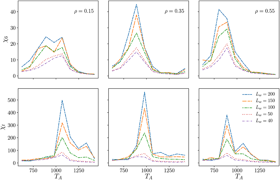
Figure 6. The susceptibilities χ₆ and χ_t of the global order parameters Ψ₆, Ψ_t, respectively. A system with parameters L = 1, 200 and ν = 48 was subdivided into square subdomains of widths L_w. For each of these subdomains the global order parameters and the susceptibilities are computed and then a variance of those measurements is taken.

4.3. Topological Defect Analysis

Two types of topological defects accompany the KTHNY melting scenario, namely dislocations and disclinations. Dislocations are translational defects, which destroy long range translational order when are isolated or free. On the other hand, disclinations are orientational defects, which destroy the long range orientational order when they are free. In a perfect 2D hexagonal crystal all atoms have six neighbors. Disclination cores have only 7 or more neighbors whereas antidisclination cores have 5 or less neighbors [35, 36]. For a 2D crystal, an isolated tightly bound 5–7 fold disclination pair is a dislocation [32]. In an imperfect solid, dislocation defects are always found in pairs because they do not destroy long range order as shown in Figure C1 for our cTRW model.

According to the KTHNY theory of defect induced melting, by increasing temperature the system first undergoes a continuous transition from a solid where only pairs of dislocations are possible, to a hexatic phase where the pairs of dislocations “unbind” spawning free dislocations (see in Figure C1 an example of how a free disclination destroys the orientational order in the cTRW model). These free dislocations result in the loss of long range translational order found in crystals. With further increase in temperature the system then undergoes another continuous transition from hexatic to liquid where the dislocations themselves unbind resulting in free disclinations and the loss of long range orientational order [37, 38].

We analyse these topological defects in our cTRW model by considering their fraction λ in the system shown in Figure 7. For each type of defect λ is their number relative to the total number of centroids. Looking sequentially at panels (a) to (d) in Figure 7 one can see that as free disclinations drop significantly there is a sharp increase of dislocations signaling the onset of the liquid-hexatic transition at around, respectively, T_A = 870, 890, 712, and 712. The hexatic phase appears once there are no free disclinations in the system. The faster decay of the free dislocations vs. the dislocation pairs that is observed by increasing T_A is indicative of the fact that free dislocations are binding together to form pairs of dislocations. Once free dislocations disappear the system has entered the solid phase. By looking at these values of T_A when free disclinations disappear (hexatic) and free dislocations disappear (solid) we are able to identify the hexatic region in the T_A − ρ parameter space as shown in Table 1.

FIGURE 7

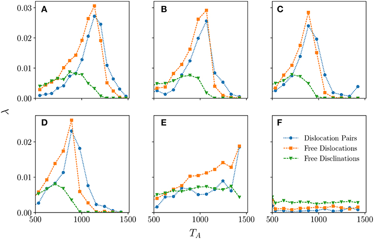
Figure 7. The fraction, λ of each of the defect types considered as a function of T_A for thermalized systems with parameters L = 1, 200 and ν = 48. The absence of free disclinations marks the transition from liquid to hexatic phase, while the absence of free dislocations is indicative of the system having transitioned into the solid phase from the hexatic phase. The panels (A–F) correspond, respectively, to ρ = 0.00, 0.15, 0.35, 0.55, 0.75, and 0.95. Defects with different number of neighbors are at least two orders of magnitude smaller than the ones drawn and we have omitted plotting them.

TABLE 1

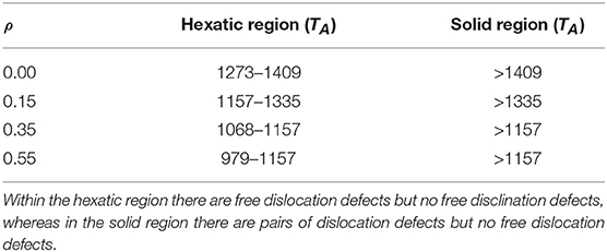
Table 1. Approximate phase regions in T_A for each value of ρ extracted from the appearance/disappearance of topological defects (see Figure 7).

Once in the solid phase with further increase of T_A the system approaches progressively the perfect crystalline arrangement by shedding paired dislocations. For the case ρ = 0.75 there is the possibility that ordered phases exist but one ought to look at values of T_A beyond those considered here. On the other hand, when ρ = 0.95 the defects show no sign of decaying. This results from the breaking down of the centroid coarse-graining analysis, which is further discussed in the following section.

4.4. Territory Fragmentation

While the previous sections have shed light on the links between the movement statistics of the walkers and the phases of the territorial system for ρ ≤ 0.55, we have a less clear picture of what occurs for large ρ. While stronger correlation implies that an animal would cross its own territory more quickly, it does not necessarily mean that the terrain is covered more efficiently. On the contrary the coverage efficiency is expected to decrease beyond a certain value of ρ as demonstrated in the ideal scenario of Figure B1. With neighboring individuals not covering efficiently their own territories, an animal spending more time at the boundaries has more chance to carve away part of the terrain recently occupied by its own neighbors. In so doing the territorial shapes become less and less convex as ρ is increased.

With further increase in ρ at any given time an animal may have its own scented territory separated into multiple islands, which are sets of contiguous lattice sites that contain the scent of one walker only. Those islands where a walker is not present are cut off quickly from its owner and get absorbed by neighboring territories. While islands get created and decay away continuously, we expect the rate at which they form to become larger than the rate at which they dissolve beyond a certain value of ρ. When that happens the centroid of an animal territory could easily be located in between multiple islands, in areas that are also covered by the scent of other individuals, or even outside its own scented region when the territory shape is highly concave. In these cases the centroid analysis, utilized in previous sections to identify the phases of the system, is not appropriate any more and there are no biological meaningful ways to define a territorial centroid.

We can, however, quantify the degree of fragmentation as a function of the system parameters by considering the ratio κ = N/I where N is the number animals in the system and I is the total number of islands. This fragmentation index is plotted in Figure 8. For low T_A values, traces of past presence of an individual get lost quickly, and thus it is not so frequent for an animal to encounter foreign scent. While such encounters increase as T_A gets larger, potentially reducing I, they are rare and are thus relatively independent of how straight the animal movement trajectories are. Beyond a certain value of T_A foreign scent encounter events become very frequent and the rate of increase is affected by the shape of the territories. For ρ ≲ 0.75 the encounters occur mainly at boundary sites and thus further increase in T_A does not change the number of islands in the system, which remains at κ = 1 when the number of islands corresponds to the number of territories. This is not the case for ρ > 0.75 where the number of islands becomes larger than N.

FIGURE 8

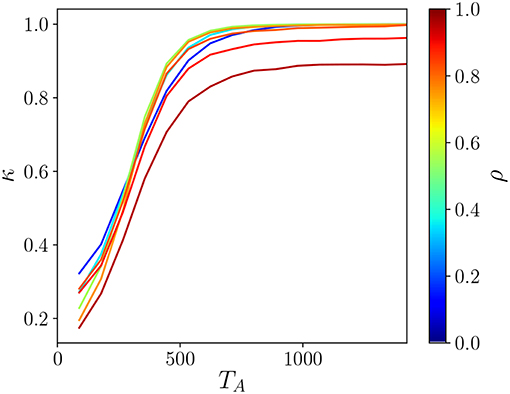
Figure 8. The fragmentation index κ as a function of the active scent time T_A for thermalized systems with parameters L = 1, 200 and ν = 48. With ρ ≲ 0.75, at low T_A values the territories are concave and as a result are more prone to fragmentation resulting in low κ. As the T_A is increased, the territories become more convex becoming more resistant to fragmentation resulting in κ = 1 for T_A ≳ 800. On the other hand, for ρ ≳ 0.75 fragmentation persists in the system regardless of T_A.

The appearance of fragmented territories for ρ ≳ 0.75 as shown in Figure 8 helps us interpret Figures 4, 5 when ρ ≥ 0.5, which indicated the presence of a fluid for any T_A. In light of Figure 8 it is clear that we cannot conclude that for larger T_A no ordered phase appears because the territory centroids are not an appropriate coarse grained representation of the animal scented territories. Although we believe that an analysis that takes into account the actual shape of the territories might help us develop other ways to identify order in fragmented terrain, we have decided not to perform such investigation here given the heavy computational cost that such a study would entail.

5. Conclusions

Territoriality is a common behavior in natural populations as it allows individual animals or family units to defend resources being food, shelter, or mates. We have studied here the case where the mechanisms through which animals defend their resources is via leaving trace of their passage on the terrain. For our theoretical analysis we have used a collective movement model recently employed to study red fox movement data [39] called the territorial random walk model. We have extended its prediction by determining how the individual movement statistics affect territory formation at the population level. And we have focused in particular on relaxing the diffusive assumption allowing the walkers to have a variable degree of correlation in their movement steps.

By studying the main parameters of the systems, namely the degree of correlation of the walk ρ and the active scent time T_A, we have brought evidence pointing to the existence of the KTHNY melting scenario with liquid, hexatic and solid phases. We have identified the coverage efficiency of an individual territory, which is controlled by ρ and T_A, as the micro level behavior that explains why different phases of territories are present at the macro level.

As the movement of the individuals becomes more correlated i.e., by increasing ρ from 0, they increase territory coverage. Individuals are able to re-scent more quickly and more readily defend their territory from neighbors. Territories are less mobile and the whole system becomes more ordered.

Beyond an intermediate degree of correlation, that is for high values of ρ, the walkers are not only inefficient at covering their own territory, but also spend more time at the borders. Their increased presence at the borders gives them more opportunities to take over neighboring territories. This results in large variation in the shape and size of territories and ultimately their fragmentation. In this scenario, the coarse grained approximation is no longer suitable to determine the spatial ordering.

Moreover, we have demonstrated how it may be useful to look at the presence of different types of topological defects to pinpoint phase transitions in the correlated territorial random walk model. As thermodynamic limits represent a big abstraction from the realm of biological systems we believe that this latter part of our analysis will be instrumental to determine empirically the spatial order of an actual population of territorial animals. With the recent development in animal tracking [40] it is in fact realistic to have in the near future simultaneous highly resolved movement data of neighboring territorial individuals from which defect densities and movement correlation statistics can be extracted.

Applications of this study extend beyond an ecological context. For example, in multi-robot online area coverage [31] tasks such as surveillance, search and harvesting [41–44] involve coordinating a large number of robots. In such cases the natural approach is to use a decentralized controller [45]. The observations and insights of this study may help refine stigmergic control systems that have been successfully demonstrated in previous studies [46, 47]. As an avenue for future research, it might be interesting to study the difference of the cTRW model on scale-free and small-world networks and compare it the bioinspired machine learning models used for semi-supervised learning [48, 49].

Data Availability

The datasets generated for this study are available on request to the corresponding author. Data used can be found at https://www.dropbox.com/sh/06ts5rwb922yqwk/AADeY66Q_7fqn5axMKcCK-Tra?dl=0.

Author Contributions

LG designed the study and wrote the paper. SS and AH created the computational code. SS analyzed the data.

Funding

LG and SS acknowledge funding from, respectively, the Engineering and Physical Research Council Grant nos. EP/I013717/1 and S108151-111.

Conflict of Interest Statement

The authors declare that the research was conducted in the absence of any commercial or financial relationships that could be construed as a potential conflict of interest.

Supplementary Material

The Supplementary Material for this article can be found online at: https://www.frontiersin.org/articles/10.3389/fphy.2019.00129/full#supplementary-material

References

1. Goychuk I, Kharchenko VO, Metzler R. How molecular motors work in the crowded environment of living cells: coexistence and efficiency of normal and anomalous transport. PLoS ONE. (2014) 9:e91700. doi: 10.1371/journal.pone.0091700

PubMed Abstract | CrossRef Full Text | Google Scholar

2. Kusumi A, Nakada C, Ritchie K, Murase K, Suzuki K, Murakoshi H, et al. Paradigm shift of the plasma membrane concept from the two-dimensional continuum fluid to the partitioned fluid: high-speed single-molecule tracking of membrane molecules. Annu Rev Biophys Biomol Struct. (2005) 34:351–78. doi: 10.1146/annurev.biophys.34.040204.144637

PubMed Abstract | CrossRef Full Text | Google Scholar

3. Kenkre VM, Giuggioli L, Kalay Z. Molecular motion in cell membranes: analytic study of fence-hindered random walks. Phys Rev E. (2008) 77:051907. doi: 10.1103/PhysRevE.77.051907

PubMed Abstract | CrossRef Full Text | Google Scholar

4. Dieterich P, Klages R, Preuss R, Schwab A. Anomalous dynamics of cell migration. Proc Natl Acad Sci USA. (2008) 105:459–63. doi: 10.1073/pnas.0707603105

PubMed Abstract | CrossRef Full Text | Google Scholar

5. Viswanathan GM, da Luz MGE, Raposo EP, Stanley HE. The Physics of Foraging: An Introduction to Random Searches and Biological Encounters. Carmbridge: Cambridge Univ. Press (2011).

Google Scholar

6. Boyer D, Crofoot MC, Walsh PD. Non-random walks in monkeys and humans. J Roy Soc Interface. (2011) 9:842–7. doi: 10.1098/rsif.2011.0582

PubMed Abstract | CrossRef Full Text | Google Scholar

7. Falcón-Cortés A, Boyer D, Giuggioli L, Majumdar SN. Localization transition induced by learning in random searches. Phys Rev Lett. (2017) 119:140603. doi: 10.1103/PhysRevLett.119.140603

PubMed Abstract | CrossRef Full Text | Google Scholar

8. Goldstein S. On diffusion by discontinuous movements, and on the telegraph equation. Q J Mech Appl Math. (1951) 4:129–56. doi: 10.1093/qjmam/4.2.129

CrossRef Full Text | Google Scholar

9. Codling EA, Planck MJ, Benhamou S. Random walk models in biology. J Roy Soc Interface. (2008) 95:813–34. doi: 10.1098/rsif.2008.0014

CrossRef Full Text | Google Scholar

10. Benhamou S. Of scales and stationarity in animal movements. Ecol Lett. (2014) 17:261–72. doi: 10.1111/ele.12225

PubMed Abstract | CrossRef Full Text | Google Scholar

11. Brown JL, Orians GH. Spacing patterns in mobile animals. Ann Rev Ecol Syst. (1970) 1:239–62. doi: 10.1146/annurev.es.01.110170.001323

CrossRef Full Text | Google Scholar

12. Burt WH. Territoriality and home range concepts as applied to mammals. J Mammal. (1943) 24:346–52.

Google Scholar

13. Maher CA, Lott DF. Definitions of territoriality used in the study of variation in vertebrate spacing systems. Anim Behav. (1995) 49:1581–97.

Google Scholar

14. Adams ES. Approaches to the study of territory size and shape. Ann Rev Ecol Syst. (2001) 32:277–303. doi: 10.1146/annurev.ecolsys.32.081501.114034

CrossRef Full Text | Google Scholar

15. Davies NB, Houston AI. Territory economics. In: Krebs JR, Davies NB, editors. Behavioural Ecology: An Evolutionary Approach, 2nd ed. Oxford: Blackwell Sci. (1984). p. 148–69.

Google Scholar

16. Gosling LM, Roberts SC. Scent-marking by male mammals: cheat-proof signals to competitors and mates. Adv Stud Behav. (2001) 30:169–217. doi: 10.1016/S0065-3454(01)80007-3

CrossRef Full Text | Google Scholar

17. Grassé PP. La reconstruction du nid et les coordinations interindividuelles chez Bellicositermes natalensis et Cubitermes sp. La théorie de la stigmergie: essai dÕinterprétation du comportement des termites constructeurs. Insec Soc. (1959) 6:41–83.

Google Scholar

18. Theraulaz G, Bonabeau E. A brief history of stigmergy. Artificial Life. (1999) 5:97–116.

PubMed Abstract | Google Scholar

19. Giuggioli L, Potts JR, Rubenstein DI, Levin SA. Stigmergy, collective actions, and animal social spacing. Proc Natl Acad Sci USA. (2013) 110:16904–9. doi: 10.1073/pnas.1307071110

PubMed Abstract | CrossRef Full Text | Google Scholar

20. Lewis MA, Murray JD. Modelling territoriality and wolf-deer interactions. Ecology. (1993) 366:738–40.

Google Scholar

21. Moorcroft PR, Lewis MA. Mechanistic Home Range Analysis. Princeton, NJ: Princeton University Press (2006).

Google Scholar

22. Giuggioli L, Potts JR, Harris S. Animal interactions and the emergence of territoriality. PLoS Comput Biol. (2011) 7:e1002008. doi: 10.1371/journal.pcbi.1002008

PubMed Abstract | CrossRef Full Text | Google Scholar

23. Giuggioli L, Kenkre VM. Consequences of animal interactions on their dynamics: emergence of home ranges and territoriality. Mov Ecol. (2014) 2:20. doi: 10.1186/s40462-014-0020-7

PubMed Abstract | CrossRef Full Text | Google Scholar

24. Alberts AC. Constraints on the design of chemical communication systems in terrestrial vertebrates. Am Nat. (1992) 139:S62–89.

Google Scholar

25. Heiblum Robles A, Giuggioli L. Phase transitions in stigmergic territorial systems. Phys Rev E. (2018) 98:042115. doi: 10.1103/PhysRevE.98.042115

CrossRef Full Text | Google Scholar

26. Halperin BI, Nelson DR. Theory of two-dimensional melting. Phys Rev Lett. (1978) 41:121–4.

Google Scholar

27. Kosterllitz DJ, Thouless JM. Ordering, metastability and phase transitions in two-dimensional systems. J Phys C Solid State Phys. (1973) 1181:1181–203.

Google Scholar

28. Young AP. Melting and the vector Coulomb gas in two dimensions. Phys Rev B. (1979) 19:1855–66.

Google Scholar

29. Giuggioli L, Abramson G, Kenkre VM, Parmenter RR, Yates TL. Theory of home range estimation from displacement measurements of animal populations. J Theor Biol. (2006) 240:126–35. doi: 10.1016/j.jtbi.2005.09.002

PubMed Abstract | CrossRef Full Text | Google Scholar

30. Chupeau M, Bénichou O, Voituriez R. Cover times of random searches. Nat Phys. (2015) 11:844. doi: 10.1038/nphys3413

CrossRef Full Text | Google Scholar

31. Giuggioli L, Arye I, Heiblum Robles A, Kaminka GA. From ants to birds: a novel bio-inspired approach to online area coverage. In: Groß R, Kolling A, Berman S, Frazzoli E, Martinoli A, Matsuno F, et al., editors. Distributed Autonomous Robotic Systems: The 13th International Symposium. Cham: Springer International Publishing (2018). p. 31–43.

Google Scholar

32. Binder K, Kob W. Glassy Materials and Disordered Solids: An Introduction to Their Statistical Mechanics. Singapore: World scientific (2011).

Google Scholar

33. Fraser DP, Zuckermann MJ, Mouritsen OG. Simulation technique for hard-disk models in two dimensions. Phys Rev A. (1990) 42:3186.

PubMed Abstract | Google Scholar

34. Jaster A. Computer simulations of the two-dimensional melting transition using hard disks. Phys Rev E. (1999) 59:2594.

Google Scholar

35. Harris WF. Disclinations. Sci Ame. (1977) 237:130–45.

Google Scholar

36. DeWit R. Relation between dislocations and disclinations. J Appl Phys. (1971) 42:3304–8.

Google Scholar

37. Qi W, Gantapara AP, Dijkstra M. Two-stage melting induced by dislocations and grain boundaries in monolayers of hard spheres. Soft Matter. (2014) 10:5449. doi: 10.1039/C4SM00125G

PubMed Abstract | CrossRef Full Text | Google Scholar

38. Quinn RA, Goree J. Experimental test of two-dimensional melting through disclination unbinding. Phys Rev E. (2001) 64:051404. doi: 10.1103/PhysRevE.64.051404

PubMed Abstract | CrossRef Full Text | Google Scholar

39. Potts JR, Harris S, Giuggioli L. Quantifying behavioral changes in territorial animals caused by sudden population declines. Am Nat. (2013) 182:E73–82. doi: 10.1086/671260

PubMed Abstract | CrossRef Full Text | Google Scholar

40. Nathan RM, Giuggioli L. A milestone for movement ecology research. Move Ecol. (2013) 1:1. doi: 10.1186/2051-3933-1-1

PubMed Abstract | CrossRef Full Text | Google Scholar

41. Schneider-Fontán M, Matarić MJ. Territorial multi-robot task division. IEEE Trans Robot Automat. (1998) 14:815–22.

Google Scholar

42. Larionova S, Almeida N, Marques L, De Almeida AT. Olfactory coordinated area coverage. Autonom Robots. (2006) 20:251–60. doi: 10.1007/s10514-006-7099-7

CrossRef Full Text | Google Scholar

43. Paull L, Saeedi S, Seto M, Li H. Sensor-driven online coverage planning for autonomous underwater vehicles. IEEE/ASME Trans Mechat. (2013) 18:1827–38. doi: 10.1109/TMECH.2012.2213607

CrossRef Full Text | Google Scholar

44. Fazli P, Davoodi A, MacKworth AK. Multi-robot repeated area coverage. Autonom Robot. (2013) 34:251–76. doi: 10.1007/s10514-012-9319-7

CrossRef Full Text | Google Scholar

45. Marjovi A, Nunes JG, Marques L, De Almeida A. Multi-robot exploration and fire searching. In: 2009 IEEE/RSJ International Conference on Intelligent Robots and Systems, IROS 2009. St. Louis, MO: IEEE. (2009). p. 1929–34. doi: 10.1109/IROS.2009.5354598

CrossRef Full Text | Google Scholar

46. Scheidt D, Stipes J. Cooperating unmanned vehicles. In: Proceedings 2005 IEEE Networking, Sensing and Control, 2005. Tucson, AZ: IEEE (2005). p. 326–31.

Google Scholar

47. Stipes J, Hawthorne R, Scheidt D, Pacifico D. Cooperative localization and mapping. In: 2006 IEEE International Conference on Networking, Sensing and Control. Fort Lauderdale, FL: IEEE (2006). p. 596–601.

Google Scholar

48. de Arruda HF, Silva FN, Costa LdF, Amancio DR. Knowledge acquisition: a complex networks approach. Inform Sci. (2017) 421:154–66. doi: 10.1016/j.ins.2017.08.091

CrossRef Full Text | Google Scholar

49. Lima TS, de Arruda HF, Silva FN, Comin CH, Amancio DR, Costa LdF. The dynamics of knowledge acquisition via self-learning in complex networks. Chaos Interdiscipl J Nonlinear Sci. (2018) 28:083106. doi: 10.1063/1.5027007

PubMed Abstract | CrossRef Full Text | Google Scholar