A Perturbative Approach to the Tunneling Phenomena

The double-well potential is a good example, where we can compute the splitting in the bound state energy of the system due to the tunneling effect with various methods, namely path-integral, WKB, and instanton calculations. All these methods are non-perturbative and there is a common belief that it is difficult to find the splitting in the energy due to the barrier penetration from a perturbative analysis. However, we will illustrate by explicit examples including singular potentials (e.g., Dirac delta potentials supported by points and curves and their relativistic extensions) it is possible to find the splitting in the bound state energies by developing some kind of perturbation method.

1. Introduction

Most real quantum mechanical systems can not be solved exactly and we usually apply some approximation methods, the most common one being perturbation theory, to get information about the energy levels and scattering amplitudes. However, not all quantum systems can be analyzed by perturbative methods. There are various class of problems where we can not deduce any information by simply using perturbation theory since these problems are inherently non-perturbative phenomena like the formation of bound states and penetration through a potential barrier. For such non-perturbative phenomenon, other tools, such as WKB [1, 2] and instanton calculations [3], are particularly useful. The particle moving in a one-dimensional anharmonic potential $V(x)=\frac{{\lambda }^2}{8}{(x^2-a^2)}^2$ is a classic example, where we can show the barrier penetration through the WKB analysis.

When the energy scale determined by the length scale a is extremely small compared with the binding energy of the system, i.e., ℏ²/2ma² << E_B, or λa² >> 1, the potential separates into two symmetrical wells with a very high barrier (see Figure 1). In this extreme regime, as a first approximation, each well has separately quantized energy levels and these energy levels are degenerate due to the symmetry. However, once the large but finite value of the coupling constant λ is taken into account, the particle initially confined to one well can tunnel to the other well so the degeneracy in the energy levels disappear. The splitting in the resulting energy levels (between the true ground state and the first excited level due to the tunneling) is given by Landau [1] and Das [2]

$\begin{array}{ll}\delta E=E_2-E_1\approx \frac{4e}{\pi }\sqrt{m\hslash }{\omega }^{3/2}aexp\left(-\frac{1}{\hslash }{S}_0\right)& (1)\end{array}$

where $S_0=\frac{2m\omega a^2}{3}$ and ${\omega }^2=\frac{{\lambda }^2{a}^2}{m}$. The above exponentially decaying factor with respect to the separation between the wells illustrates the tunneling effect. The true ground state corresponds to a symmetric combination and the excited level corresponds to the anti-symmetric combination of the WKB corrected wave functions.

FIGURE 1

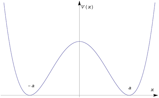
Figure 1. Anharmonic potential.

Among the exactly solvable potentials in quantum mechanics, Dirac delta well potentials are the most well-known text book example [4]. Moreover, it has been studied extensively in mathematical physics literature from the different point of views, in particular in the context of self-adjoint extension of symmetric operators [5]. Although it is easier to define it rigorously in one dimension through the quadratic forms, one possible way to define it in higher dimensions is to consider the free symmetric Hamiltonian defined on a dense domain excluding the point, where the support of the Dirac delta function is located, and then apply the self-adjoint extension techniques developed by J. Von Neumann [see the monograph [6] for the details and also for the historical development with extensive literature in the subject]. Then, the formal (or heuristic) definition of one-dimensional Dirac delta potentials in the physics literature is understood as the one particular choice among the four parameter family of the self-adjoint operators, where the matching conditions of the wave function are just obtained from the boundary conditions (which define the domain of our self-adjoint operator) constructed through the extension theory. Another way to introduce these point interactions uses the resolvent method, developed by M. Krein, and it is based on the observation that for such type of potentials the resolvent can be found explicitly and expressed via the so-called Krein's formula [7]. Within this approach, the Hamiltonian for point interaction (in two and three dimensions) is first approximated (regularized) by a properly chosen sequence of self-adjoint operators H_ϵ and then the coupling constant (or strength) of the potential is assumed to be a function of the parameter ϵ in such a way that one obtains a non-trivial limit. This convergence is actually in the strong resolvent sense, so the limit operator is self-adjoint [8]. Since the Dirac delta potentials in two and three dimensions require renormalization, it is usually considered as a toy model for the renormalization originally developed in quantum field theories and it helps us to better understand the various ideas in field theory such as renormalization group and asymptotic freedom [9–12]. Furthermore, point like Dirac delta interactions have been also extended to various generalizations. For our approach, to illustrate the main ideas, we are mainly concerned with the delta potentials supported by points on flat and hyperbolic manifolds [13–15], and delta potentials supported by curves in flat spaces, and its various relativistic extensions in flat spaces [16–19].

In this paper, we explicitly demonstrate for a class of singular potential problems that the splitting in the energy levels due to the tunneling can be realized by simply developing some kind of perturbation theory. We have two basic assumptions here: (1) Binding energies of individual Dirac delta potentials are all different. Otherwise we need to employ degenerate perturbation theory. Actually, we briefly discus a particular degenerate case, namely the two center case in two dimensions to compare with the double well potential. (2) The support of singular interactions are sufficiently separated from one another, as a result the bound state wave functions decay rapidly over the distances between them.

All the findings about the splitting in the bound state energies for singular potentials on hyperbolic manifolds treated here could be applied to the two dimensional systems such as graphite sheets. We can model impurities in these systems as attractive centers in some approximation and these sheets can be put in various shapes. This is especially true for surfaces with variable sectional curvature which is not completely negative. The negatively curved surfaces, of course, cannot be realized as embedded surfaces in three dimensions due to Hilbert's well-known theorem. Nevertheless, we may envisage these models as an effective description of unusual quasi-particle states of some two dimensional systems. Due to the interactions, the system may develop a gap in the spectrum and the effective description may well be best understood through a negative sectional curvature space. Moreover, the problems related with point interactions on Lobachevsky plane have been studied from different points of view [20, 21]. The point interactions can be extended on more general class of manifolds as well [22]. In particular, they have been studied on some particular surfaces in ℝ³, namely on the infinite planar strip as a natural model for quantum wires containing impurities [23] and on the torus [24]. A more heuristic approach for point interactions on Riemannian manifolds has been constructed through the heat kernel in Altunkaynak et al. [13] and Erman and Turgut [14]. The physical motivation behind studying the Dirac delta potentials supported by curves is based on the need for modeling semiconductor wires [25]. They could be considered as a toy model for electrons confined to narrow tube-like regions.

The paper is organized as follows: In section 2, we formally summarize the resolvent formulae, called Krein's formulae, for Hamiltonians perturbed by singular potentials including Dirac delta potentials supported by points and curves. The principal matrices for each case are given explicitly. The relativistic and the field theoretical extension of it has been also reviewed in the subsections of this section. In section 3, we briefly discuss the analytic structure of the principal matrix and the bound state spectrum for such type of singular interactions. In Section 4, we discuss how the off-diagonal terms of the principal matrix change in the tunneling regime. section 5 and section 6 contain the formulation of the perturbative analysis and explicit calculations of the splitting in the bound state energy when these singular interactions are far away from each other, which is the main result of the paper. We finally discuss the degenerate case and wave functions, and compare the one dimensional results with the exact result in section 7.

2. Krein's Formulae for Free Hamiltonians Perturbed by Singular Interactions

Before we are going to discuss the perturbative analysis of singular interactions for large separations of the support of the potentials, we first present the basic results about our formulation of the singular Hamiltonians. In this paper, we are mainly concerned with the Dirac delta potentials supported by finitely many points and finitely many curves in flat spaces, and their extension to the hyperbolic manifolds. Moreover, we also consider some relativistic extensions of these singular interactions.

Since we study the spectral properties of different kinds of Dirac delta potentials, we first introduce the notation for Dirac delta functions of interest. The Dirac delta distribution δ_a supported by a point a in ℝⁿ is defined as a continuous linear functional whose action on the test functions ψ is given by

$\begin{array}{ll}\langle {\delta }_a,\psi \rangle =\psi (\text{a}).& (2)\end{array}$

Similarly, Dirac delta distribution δ_γ supported by a curve Γ in ℝⁿ is defined as a continuous linear functional whose action on the test functions ψ is given by Appel [26]

$\begin{array}{ll}\langle {\delta }_{\gamma },\psi \rangle ={\displaystyle {\int }_{\Gamma }}ds\psi (\gamma (s)).& (3)\end{array}$

The left hand sides in the definitions (2) and (3) can be expressed in the Dirac's bra-ket notation, most common in physics literature, as 〈a|ψ〉 and 〈γ|ψ〉, respectively.

As we have already emphasized in the introduction, there are several ways to define rigorously the Hamiltonian for Dirac delta potentials. Here, we start with a finite rank perturbations of self-adjoint free Hamiltonian H₀ (e.g., $H_0=P^2/2m$ in the non-relativistic case and $H_0=\sqrt{P^2+m^2}$ in the semi-relativistic case):

$\begin{array}{ll}H=H_0-{\displaystyle \sum _{i=1}^N}{\lambda }_i\langle {\phi }_i,.\rangle {\phi }_i,& (4)\end{array}$

where ${\phi }_i\in {H}$ and 〈., .〉 denotes the sesqui-linear inner product in the Hilbert space ${H}$. Then, it is well-known that the resolvent of H can be explicitly found in terms of the resolvent of the free part by simply solving the inhomogenous equation [7]

$\begin{array}{ll}(H-z)\psi =\rho ,& (5)\end{array}$

for a given $\rho \in {H}$ and ψ ∈ D(H₀) = D(H). Here D stands for the domain of the operator and we assume that ℑ(z) > 0. It is well-known that H is self-adjoint on D(H₀) due to the Kato-Rellich theorem [5]. The resolvent of H could be found in two steps: First, we apply the resolvent of the free part to the Equation (5)

$\begin{array}{ll}{(H_0-z)}^{-1}\rho =\psi -{\displaystyle \sum _{i=1}^N}{\lambda }_i\langle {\phi }_i,\psi \rangle {(H_0-z)}^{-1}{\phi }_i,& (6)\end{array}$

and project this on the vector φ_j, we can then find the solution 〈φ_i, ψ〉 so that the resolvent $R_z(H)={(H-z)}^{-1}$ of the Hamiltonian H at z is:

$\begin{array}{ll}{R}_z(H)=R_z(H_0)+{\displaystyle \sum _{i,j=1}^N}{R}_z(H_0){\phi }_i{[{\Phi }^{-1}(z)]}_{ij}\langle R_{\bar{z}}(H_0){\phi }_j,.\rangle ,& (7)\end{array}$

where

$\begin{array}{ll}{\Phi }_{ij}(z)=\{\begin{array}{cc}\frac{1}{{\lambda }_i}-\langle {\phi }_i,R_z(H_0){\phi }_i\rangle \hfill & \text{if }i=j\hfill \\ -\langle {\phi }_i,R_z(H_0){\phi }_j\rangle \hfill & \text{if }j\ne j^{\prime }\hfill \end{array}.\hfill & (8)\end{array}$

Actually, the resolvent formula (7) is valid even in the case where the vectors φ_i's do not belong to the Hilbert space. Such perturbations represent the singular type of interactions, e.g., Dirac delta potentials supported by points or curves [6, 16]. In Dirac's bra-ket notation, one can also express the above resolvent formula as:

$\begin{array}{ll}{R}_z(H)=R_z(H_0)+{\displaystyle \sum _{i,j=1}^N{R}_z}(H_0)|{\phi }_i\rangle {[{\Phi }^{-1}(z)]}_{ij}\langle {\phi }_j|R_z(H_0).& (9)\end{array}$

The explicit expression of the resolvent (7) or (9) is known as Krein's resolvent formula. Alternatively, these singular interactions can be defined directly through von Neumann's self-adjoint extension theory (or quadratic forms in some cases). Since our aim is the spectral behavior and especially the bound state problem of such singular interactions, Krein's explicit formula is much more useful. Throughout the paper, following the terminology introduced by Rajeev [27] we call the matrix Φ as the principal matrix (this is equivalent to the matrix Γ used in Albeverio et al. [6]).

Actually, one can also develop the above resolvent formula (9) to relativistic and field theoretical extensions of the singular models, as we will discuss in the next subsections. Let us now summarize explicitly the resolvent formulae and principal matrices in all classes of singular interactions that we are going to discuss in this paper:

2.1. Point-Like Dirac Delta Interactions in ℝ

The Hamiltonian for the non-relativistic particle moving in fixed N point like Dirac delta potentials in one dimension can be expressed in terms of the formal projection operators given by the Dirac kets |a_i〉

$\begin{array}{ll}H=H_0-{\displaystyle \sum _{i=1}^N{\lambda }_i}|a_i\rangle \langle a_i|,& (10)\end{array}$

where H₀ is the non-relativistic free Hamiltonian, and λ_j's are positive constants, called coupling constants or strengths of the potential. Throughout this paper, we will use the units such that ℏ = 2m = 1 for non-relativistic cases and ℏ = c = 1 only for the relativistic case. Since we have fairly complicated expressions, this simplifies our writing, hoping that this does not lead to any further complications. It is well-known in the literature that there are different ways to make sense of this formal Hamiltonian in a mathematically rigorous way [strictly speaking, the above expression (10) has no meaning as an operator in L²(ℝ)]. Let us define R_z(H): = R(z) and R_z(H₀): = R₀(z) for simplicity. Even though it is hard to make sense of the Hamiltonian, one can find the resolvent of this formal operator algebraically and the result is consistent with the one given by a more rigorous formulation. Choosing φ_i as the Dirac kets |a_i〉 formally in the previous section, the resolvent is explicitly given by

$\begin{array}{ll}R(z)=R_0(z)+{\displaystyle \sum _{i,j=1}^N}{R}_0(z)\left|a_i\rangle {[{\Phi }^{-1}(E)]}_{ij}\langle a_j\right|R_0(z),& (11)\end{array}$

where Φ is an N × N matrix

$\begin{array}{ll}{\Phi }_{ij}(z)=\{\begin{array}{cc}\frac{1}{{\lambda }_i}-R_0(a_i,a_i;z)& \text{if }i=j\\ -R_0(a_i,a_j;z)& \text{if }i\ne j\end{array}.& (12)\end{array}$

Here $R_0(a_i,a_j;z)=\langle a_i|{(H_0-z)}^{-1}|a_j\rangle$ is the free resolvent kernel. It is useful to express the principal matrix in terms of the heat kernel K_t(a_i, a_j) - the fundamental solution to the Cauchy problem associated with the heat equation—using

$\begin{array}{l}{R}_0(a_i,a_j;z)=\langle a_i|{(H_0-z)}^{-1}|a_j\rangle =\langle a_i|{\displaystyle {\int }_0^{\infty }}dt{e}^{t(H_0-z)}|a_j\rangle \\ ={\displaystyle {\int }_0^{\infty }}dt{K}_t(a_i,a_j)e^{tz}.& (13)\end{array}$

Then, we obtain

$\begin{array}{ll}{\Phi }_{ij}(z)=\{\begin{array}{cc}\frac{1}{{\lambda }_i}-{\int }_0^{\infty }dt{K}_t(a_i,a_i)e^{tz}& \text{if }i=j\\ -{\int }_0^{\infty }dt{K}_t(a_i,a_j)e^{tz}\hfill & \text{if }i\ne j\end{array}.& (14)\end{array}$

These expressions should be considered as analytical continuations of the formulae beyond their regions of convergence in the variable z. From the resolvent (11), one can also write down the resolvent kernel

$\begin{array}{ll}R(x_1,x_2;z)=R_0(x_1,x_2;z)+{\displaystyle \sum _{i,j=1}^N}{R}_0(x_1,a_i;z){\left[{\Phi }^{-1}\right]}_{ij}{R}_0(a_j,x_2;z).& (15)\end{array}$

Using the explicit expression of the integral kernel of the free resolvent

$\begin{array}{ll}{R}_0(x,y;z)=\frac{i}{2\sqrt{z}}{e}^{i\sqrt{z}|x-y|},& (16)\end{array}$

we have

$\begin{array}{ll}{\Phi }_{ij}(z)=\{\begin{array}{cc}\frac{1}{{\lambda }_i}-\frac{i}{2\sqrt{z}}\hfill & \text{if }i=j\hfill \\ -\frac{i}{2\sqrt{z}}{e}^{i\sqrt{z}|a_i-a_j|}\hfill & \text{if }i\ne j\hfill \end{array}.\hfill & (17)\end{array}$

Here $\sqrt{z}$ is defined as the unambiguous square root of z with $\Im \sqrt{z}$ is positive. Since we study the bound state spectrum, it is sometimes convenient to express the above matrix Φ(z) in terms of a real positive variable $\nu =-i\sqrt{z}$, i.e.,

$\begin{array}{ll}{{\Phi }_{ij}\left(z\right)|}_{z=-v^2}:={\Phi }_{ij}(\nu )=\{\begin{array}{cc}\frac{1}{{\lambda }_i}-\frac{1}{2\nu }\hfill & \text{if }i=j\hfill \\ -\frac{1}{2\nu }{e}^{-\nu |a_i-a_j|}\hfill & \text{if }i\ne j\hfill \end{array}.\hfill & (18)\end{array}$

2.2. Point-Like Dirac Delta Interactions in ℝ² and ℝ³

We assume that the centers of the Dirac delta potentials do not coincide, that is, a_i ≠ a_j whenever i ≠ j. If we follow the same steps outlined above, we find exactly the same formal expression for the resolvent for point interactions in two and three dimensions except for the fact that the explicit expression of the integral kernel of the free resolvent in ℝ² and ℝ³ [6] are given by

$\begin{array}{ll}{R}_0({\text{r}}_1,{\text{r}}_2;z)=\frac{i}{4}{H}_0^{(1)}(\sqrt{z}|{\text{r}}_1-{\text{r}}_2|),\hfill & (19)\end{array}$

$\begin{array}{ll}{R}_0({\text{r}}_1,{\text{r}}_2;z)=\frac{e^{i\sqrt{z}|{\text{r}}_1-{\text{r}}_2|}}{4\pi |{\text{r}}_1-{\text{r}}_2|},\hfill & (20)\end{array}$

respectively. Here $H_0^{(1)}$ is the Hankel function of the first kind of order zero and $\Im \sqrt{z}>0$. Unfortunately, the diagonal part of the free resolvent kernels are divergent so the diagonal part of the principal matrices are infinite. This is clear for the three dimensional case from the asymptotic behavior of the Hankel function [28]

$\begin{array}{ll}{H}_0^{(1)}(x)\approx -\frac{2i}{\pi }log(2/x),\hfill & (21)\end{array}$

as x → 0.

This difficulty can be resolved by the so-called regularization and renormalization method. Instead of starting with the higher dimensional version of the formal Hamiltonian (10), we first consider the regularized Hamiltonian through the heat kernel

$\begin{array}{ll}{H}_{ϵ}=H_0-{\displaystyle \sum _{i=1}^N}{\lambda }_i(ϵ)|{\text{a}}_{\text{i}}^{ϵ}\rangle \langle {\text{a}}_{\text{i}}^{ϵ}|,\hfill & (22)\end{array}$

where $\langle \text{r}|{{\text{a}}_{\text{i}}}^{ϵ}\rangle =K_{ϵ/2}(\text{r},{\text{a}}_{\text{i}})$. The heat kernel associated with the heat equation ${\nabla }^2\psi -\frac{\partial \psi }{\partial t}=0$ in ℝⁿ is given by

$\begin{array}{ll}{K}_t({\text{r}}_1,{\text{r}}_2)=\frac{1}{{(4\pi t)}^{n/2}}{e}^{-\frac{|{\text{r}}_1-{\text{r}}_2{|}^2}{4t}}.\hfill & (23)\end{array}$

It is important to note that

$\begin{array}{ll}{K}_{ϵ/2}(\text{r},{\text{a}}_{\text{i}})\to \delta (\text{r}-{\text{a}}_{\text{i}}),\hfill & (24)\end{array}$

as ϵ → 0⁺ in the distributional sense. Then, we can easily find the resolvent kernel associated with the regularized Hamiltonian (22)

$\begin{array}{l}{R}_{ϵ}({\text{r}}_1,{\text{r}}_2;z)=R_0({\text{r}}_1,{\text{r}}_2;z)\hfill \\ +{\displaystyle \sum _{i,j=1}^N}{R}_0({\text{r}}_1,{\text{a}}_{\text{i}};z){\left[{\Phi }_{ϵ}(z)\right]}_{ij}^{-1}{R}_0({\text{a}}_{\text{j}},{\text{r}}_2;z),\hfill & (25)\end{array}$

where

$\begin{array}{ll}{\left[{\Phi }_{ϵ}(z)\right]}_{ij}=\{\begin{array}{cc}\frac{1}{{\lambda }_i(ϵ)}-{\int }_0^{\infty }dt{K}_{t+ϵ}({\text{a}}_{\text{i}},{\text{a}}_{\text{i}})e^{tz}\hfill & \text{if }i=j\hfill \\ -{\int }_0^{\infty }dt{K}_{t+ϵ}({\text{a}}_{\text{i}},{\text{a}}_{\text{j}})e^{tz}\hfill & \text{if }i\ne j\hfill \end{array}.\hfill & (26)\end{array}$

If we choose

$\begin{array}{ll}\frac{1}{{\lambda }_i(ϵ)}={\displaystyle {\int }_0^{\infty }}dt{K}_{t+ϵ}({\text{a}}_{\text{i}},{\text{a}}_{\text{i}})e^{t{E}_B^i}\hfill & (27)\end{array}$

where $E_B^i<0$ (the spectrum of the free Hamiltonian only includes the continuous spectrum: [0, ∞]) is the bound state energy of the particle to the i th center in the absence of all the other centers and take the formal limit ϵ → 0⁺ we find

$\begin{array}{l}R({\text{r}}_1,{\text{r}}_2;z)=R_0({\text{r}}_1,{\text{r}}_2;z)\hfill \\ +{\displaystyle \sum _{i,j=1}^N}{R}_0({\text{r}}_1,{\text{a}}_{\text{i}};z){\left[\Phi (z)\right]}_{ij}^{-1}{R}_0({\text{a}}_{\text{j}},{\text{r}}_2;z),\hfill & (28)\end{array}$

where

$\begin{array}{ll}{\Phi }_{ij}(z)=\{\begin{array}{cc}{\int }_0^{\infty }dt{K}_t({\text{a}}_{\text{i}},{\text{a}}_{\text{i}})\left(e^{t{E}_B^i}-e^{tz}\right)\hfill & \text{if }i=j\hfill \\ -{\int }_0^{\infty }dt{K}_t({\text{a}}_{\text{i}},{\text{a}}_{\text{j}})e^{tz}\hfill & \text{if }i\ne j\hfill \end{array}.\hfill & (29)\end{array}$

From the explicit form of the heat kernel formula (23), we obtain

$\begin{array}{ll}{\Phi }_{ij}(z)=\{\begin{array}{cc}\frac{1}{2\pi }log\left(-i\sqrt{z/|E_B^i|}\right)\hfill & \text{if }i=j\hfill \\ -\frac{i}{4}{H}_0^{(1)}(\sqrt{z}|{\text{a}}_{\text{i}}-{\text{a}}_{\text{j}}|)\hfill & \text{if }i\ne j\hfill \end{array},\hfill & (30)\end{array}$

in two dimensions and

$\begin{array}{ll}{\Phi }_{ij}\left(z\right)=\{\begin{array}{cc}\frac{\left(-i\sqrt{z}-\sqrt{|E_B^i|}\right)}{4\pi }\hfill & \text{if }i=j\hfill \\ -\frac{e^{i\sqrt{z}|{\text{a}}_{\text{i}}-{\text{a}}_{\text{j}}|}}{4\pi |{\text{a}}_{\text{i}}-{\text{a}}_{\text{j}}|}\hfill & \text{if }i\ne j\hfill \end{array},\hfill & (31)\end{array}$

in three dimensions.

Since we deal with the bound states in this paper, it is convenient to express the principal matrices in terms of the real positive variable $\nu =-i\sqrt{z}$:

$\begin{array}{ll}{\Phi }_{ij}(z){|}_{z=-{\nu }^2}=\{\begin{array}{cc}\frac{1}{2\pi }log(\nu /\sqrt{|E_B^i|})\hfill & \text{if }i=j\hfill \\ -\frac{1}{2\pi }{K}_0(\nu |{\text{a}}_{\text{i}}-{\text{a}}_{\text{j}}|)\hfill & \text{if }i\ne j\hfill \end{array},\hfill & (32)\end{array}$

in two dimensions and

$\begin{array}{ll}{\Phi }_{ij}(z){|}_{z=-{\nu }^2}=\{\begin{array}{cc}\frac{\left(\nu -\sqrt{|E_B^i|}\right)}{4\pi }\hfill & \text{if }i=j\hfill \\ -\frac{e^{-\nu |{\text{a}}_{\text{i}}-{\text{a}}_{\text{j}}|}}{4\pi |{\text{a}}_{\text{i}}-{\text{a}}_{\text{j}}|}\hfill & \text{if }i\ne j\hfill \end{array},\hfill & (33)\end{array}$

in three dimensions. Here we have used $K_0(z)=\frac{i\pi }{2}{H}_0^1(iz)$ with −π < arg(z) < π/2 and K₀(z) is the modified Bessel function of the third kind [28].

2.3. Point-Like Dirac Delta Interactions in ℍ² and ℍ³

Here we assume that the particle is intrinsically moving in the manifold. Our heuristic approach to study such type of interactions on Riemannian manifolds is based on the idea of using the heat kernel as a regulator for point interactions on manifolds [13, 14]. Thanks to the fact (24), the regularized interaction is chosen as the heat kernel on Riemannian manifolds. Once we have regularized the Hamiltonian, one can follow essentially the same steps outlined in the previous section, and obtain exactly the same form of the resolvent and principal matrix as in (28) and (29), respectively. In this paper, we only consider the particular class of Riemannian manifolds, namely two and three dimensional hyperbolic manifolds for simplicity. The heat kernel on hyperbolic manifolds of constant sectional curvature −κ² can be analytically calculated and given by Grigoryan [29]

$\begin{array}{ll}{K}_t(x,y)=\{\begin{array}{cc}\frac{\sqrt{2}}{\kappa }\frac{1}{{(4\pi t)}^{3/2}}{e}^{-{\kappa }^{2}t/4}{\displaystyle {\int }_{\kappa d(x,y)}^{\infty }}ds\frac{s{e}^{-s^2/4{\kappa }^{2}t}}{\sqrt{coshs-cosh\kappa d(x,y)}}\hfill & \text{ for }n=2\hfill \\ \frac{\kappa d(x,y)}{{(4\pi t)}^{3/2}sinh\kappa d(x,y)}{e}^{-{\kappa }^{2}t-\frac{d^2(x,y)}{4t}}\hfill & \text{ for }n=3,\hfill \end{array}\hfill & (34)\end{array}$

where d(x, y) is the geodesic distance between the points x and y on the manifold. The explicit form of the principal matrix in ℍ³ can then be easily evaluated [15]:

$\begin{array}{ll}{\Phi }_{ij}\left(z\right)=\{\begin{array}{cc}\frac{1}{4\pi }\left(\sqrt{{\kappa }^2-z}-\sqrt{{\kappa }^2-E_B^i}\right)\hfill & \text{if }i=j\hfill \\ -\left(\frac{\kappa exp\left(-d\left(a_i,a_j\right)\sqrt{{\kappa }^2-z}\right)}{4\pi sinh\left(\kappa d\left(a_i,a_j\right)\right)}\right)\hfill & \text{if }i\ne j.\hfill \end{array}\hfill & (35)\end{array}$

Similarly, the principal matrix in ℍ² can simply be evaluated by interchanging the order of integration with respect to t and s

$\begin{array}{ll}{\Phi }_{ij}\left(z\right)=\{\begin{array}{cc}\frac{1}{2\pi }\left[\psi \left(\frac{1}{2}+\sqrt{-\frac{z}{{\kappa }^2}+\frac{1}{4}}\right)-\psi \left(\frac{1}{2}+\sqrt{-\frac{E_B^i}{{\kappa }^2}+\frac{1}{4}}\right)\right]\hfill & \text{if }i=j\hfill \\ -\frac{1}{2\pi }{Q}_{\frac{1}{2}+\sqrt{-\frac{z}{{\kappa }^2}+\frac{1}{4}}}(cosh(\kappa d(a_i,a_j)))\hfill & \text{if }i\ne j,\hfill \end{array}\hfill & (36)\end{array}$

where ψ is the digamma function with its integral representation [28]

$\begin{array}{ll}\psi \left(w\right)={\displaystyle {\int }_0^{\infty }}\left(\frac{e^{-t}}{t}-\frac{e^{-tw}}{1-e^{-t}}\right)dt,\hfill & (37)\end{array}$

for ℜ(w) > 0, and Q is the Legendre function of second type [28] with its integral representation

$\begin{array}{ll}{Q}_{\alpha }(cosha)={\displaystyle {\int }_a^{\infty }}\frac{e^{-(\alpha +\frac{1}{2})r}}{\sqrt{2coshr-2cosha}}dr,\hfill & (38)\end{array}$

for real and positive a and ℜ(α) > −1.

Since the spectrum of the free Hamiltonian in ℍⁿ includes only the continuous part starting from (n − 1)²κ²/4, it is natural to assume $E_B^i<{(n-1)}^2{\kappa }^2/4$.

2.4. Two Types of Relativistic Extensions of Point-Like Dirac Delta Interactions

We first consider the so-called semi-relativistic Salpeter type free Hamiltonian (also known as relativistic spin zero Hamiltonian) perturbed by point like Dirac delta potentials in one dimension. This problem for the single center case has been first studied in Albeverio and Kurasov [30] from the self-adjoint extension point of view. The formal Hamiltonian is exactly in the same form as in (10), except for the free part

$\begin{array}{ll}H=\sqrt{-\frac{d^2}{d{x}^2}+m^2}-{\displaystyle \sum _{i=1}^N}{\lambda }_i|a_i\rangle \langle a_i|,\hfill & (39)\end{array}$

in the units where ℏ = c = 1. This non-local operator is a particular case of pseudo-differential operators and defined in momentum space as multiplication by $\sqrt{p^2+m^2}$ [31], which is known as the symbol of the operator. After following the renormalization procedure outlined above for the point interactions in two and three dimensions, the resolvent and the principal matrix is exactly the same form as in (28) and (29), respectively. However, the explicit expression of the heat kernel in this case is given by Lieb and Loss [31]

$\begin{array}{ll}{K}_t\left(x,y\right)=\frac{mt}{\pi \sqrt{{\left(x-y\right)}^2+t^2}}{K}_1\left(m\sqrt{{(x-y)}^2+t^2}\right),\hfill & (40)\end{array}$

where K₁ is the modified Bessel function of the first kind. Due to the short-time asymptotic expansion

$\begin{array}{ll}{K}_1(mt)~\frac{1}{mt},\hfill & (41)\end{array}$

the diagonal term in the principal matrix (29) is divergent. In contrast to the one-dimensional case for point Dirac delta potentials, this problem therefore requires renormalization, as noticed by Erman et al. [18] and Al-Hashimi et al. [32]. Choosing the coupling constants as in (27) by substituting the heat kernel (40) and taking the limit ϵ → 0⁺, we obtain the resolvent in the form of the Krein's formula (11). The explicit form of the diagonal principal matrix is given by Erman et al. [18]

$\begin{array}{ll}{\Phi }_{ii}(z)=\phi (E_B^i)-\phi (z),\hfill & (42)\end{array}$

where

$\begin{array}{ll}\phi \left(z\right)=\frac{z}{\pi \sqrt{m^2-z^2}}\left(\frac{\pi }{2}+arctan\frac{z}{\sqrt{m^2-z^2}}\right).\hfill & (43)\end{array}$

Its off-diagonal part is given by

$\begin{array}{ll}{\Phi }_{ij}(z)=\{\begin{array}{cc}-\frac{1}{\pi }{\int }_m^{\infty }d\mu e^{-\mu |a_i-a_j|}\frac{\sqrt{{\mu }^2-m^2}}{{\mu }^2-m^2+z^2}\hfill & \text{if }\Re z<0\hfill \\ -i\frac{e^{i\sqrt{z^2-m^2}|a_i-a_j|}}{\sqrt{1-\frac{m^2}{z^2}}}-\frac{1}{\pi }{\int }_m^{\infty }d\mu e^{-\mu |a_i-a_j|}\frac{\sqrt{{\mu }^2-m^2}}{{\mu }^2-m^2+z^2}\hfill & \text{if }\Re z>0\hfill \end{array},\hfill & (44)\end{array}$

where $E_B^i$ is the bound state energy to the i th center in the absence of all the other centers. Since the spectrum of the free Hamiltonian includes only the continuous spectrum starting from m, it is natural to expect that $E_B^i<m$.

An alternative relativistic model can be introduced from a field theory perspective in two dimensions. If we take very heavy particles interacting with a light particle, in the extreme limit of static heavy particles one recovers the following model:

$\begin{array}{l}H={\displaystyle \iint { }_{{ℝ}^2}}\frac{d^2\text{p}}{{(2\pi )}^2}\sqrt{({\text{p}}^2+m^2)}{a}^{†}(\text{p})a(\text{p})\hfill \\ -{\displaystyle \sum _{i=1}^N}{\lambda }_i{\varphi }^{(-)}({\text{a}}_{\text{i}}){\varphi }^{(+)}({\text{a}}_{\text{i}}),\hfill & (45)\end{array}$

where a_i refer to the locations of static heavy particles. Here

$\begin{array}{l}{\varphi }^{(+)}(\text{x})={\displaystyle \iint { }_{{ℝ}^2}}\frac{d^2\text{p}}{{(2\pi )}^2}\frac{e^{i\text{p}·\text{x}}}{\sqrt{2}{({\text{p}}^2+m^2)}^{1/4}}a(\text{p})\text{ and}\hfill \\ {\varphi }^{(-)}= {\varphi }^{(+)}{ }^{†},\hfill & (46)\end{array}$

where † denotes the adjoint. Since this model was worked out in Dogan and Turgut [17], we will be content with the resulting formulae only referring to the original paper for the details. We can compute the diagonal principal matrix as

$\begin{array}{ll}{\Phi }_{ii}(z)=\frac{1}{2\pi }ln\left(\frac{m-z}{m-E_B^i}\right),\hfill & (47)\end{array}$

and the off-diagonal part as

$\begin{array}{ll}{\Phi }_{ij}(z)=-\frac{1}{2\pi }{\displaystyle {\int }_0^{\infty }}\frac{ds}{{(s^2+1)}^{1/2}}{e}^{-|{\text{a}}_{\text{i}}-{\text{a}}_{\text{j}}|[m{(s^2+1)}^{1/2}-zs]},\hfill & (48)\end{array}$

for −m < ℜ(z) < m. Moreover, the binding energy of the single center should satisfy $-m<E_B^i<m$, and the lower bound is due to the stability requirement, to prevent pair creation to reduce the energy further thus rendering the model unrealistic in single particle sector.

2.5. Dirac Delta Interactions Supported by Curves in ℝ² and in ℝ³

We consider N Dirac delta potentials supported by non-intersecting smooth curves ${\gamma }_{\text{j}}:\left[0,L_j\right]\to {ℝ}^n$ of finite length L_j (n = 2, 3). Each curve is assumed to be simple, i.e., γ_j(s₁) ≠ γ_j(s₂) whenever s₁ ≠ s₂, where s₁, s₂ ∈ (0, L_j). Our formulation also allows the simple closed curves.

The Hamiltonian of the system is given by

$\begin{array}{ll}H=H_0-{\displaystyle \sum _{i=1}^N\frac{{\lambda }_i}{L_i}}|{\gamma }_i\rangle \langle {\gamma }_i|,\hfill & (49)\end{array}$

where $\langle {\gamma }_{\text{i}}|\text{r}\rangle ={\int }_{{\Gamma }_i}ds\delta (\text{r}-{\gamma }_{\text{i}}(s))$. Then, the Schrödinger equation (H|ψ〉 = E|ψ〉) associated with this Hamiltonian is

$\begin{array}{l}-{\nabla }^2\psi (\text{r})-{\displaystyle \sum _{i=1}^N}\frac{{\lambda }_i}{L_i}{\displaystyle {\int }_{{\Gamma }_i}}d{s}_i\delta (\text{r}-{\gamma }_{\text{i}}(s_i)){\displaystyle {\int }_{{\Gamma }_i}}d{s}_i^{\prime }\psi ({\gamma }_{\text{i}}(s_i^{\prime }))\\ =E\psi (\text{r}).\hfill & (50)\end{array}$

In contrast to the point-like Dirac delta interactions, this equation is a generalized Schrödinger equation in the sense that it is non-local. The resolvent kernel of the above Hamiltonian is explicitly given in the same form associated with point like Dirac delta potentials, namely

$\begin{array}{l}R({\text{r}}_1,{\text{r}}_2;z)=R_0({\text{r}}_1,{\text{r}}_2;z)\hfill \\ +{\displaystyle \sum _{i,j=1}^N}\frac{1}{\sqrt{L_i{L}_j}}{R}_0({\text{r}}_1,{\gamma }_{\text{i}};z){\left[\Phi (z)\right]}_{ij}^{-1}{R}_0({\gamma }_{\text{j}},{\text{r}}_2;z),\hfill & (51)\end{array}$

where

$\begin{array}{ll}{\Phi }_{ij}(z)=\{\begin{array}{cc}\frac{1}{{\lambda }_i}-\frac{1}{L_i}\langle {\gamma }_{\text{i}}|R_0(z)|{\gamma }_{\text{i}}\rangle \hfill & \text{if }i=j\hfill \\ -\frac{1}{\sqrt{L_i{L}_j}}\langle {\gamma }_{\text{i}}|R_0(z)|{\gamma }_{\text{j}}\rangle \hfill & \text{if }i\ne j\hfill \end{array},\hfill & (52)\end{array}$

or if we express it in terms of the heat kernel

$\begin{array}{ll}{\Phi }_{ij}(z)=\{\begin{array}{cc}\frac{1}{{\lambda }_i}-\frac{1}{L_i}{\iint }_{{\Gamma }_i\times {\Gamma }_i}d{s}_{i}d{s}_i^{\prime }{\int }_0^{\infty }dt{e}^{tz}{K}_t({\gamma }_{\text{i}}(s_i),{\gamma }_{\text{i}}(s_i^{\prime }))\hfill & \text{if }i=j\hfill \\ -\frac{1}{\sqrt{L_i{L}_j}}{\iint }_{{\Gamma }_i\times {\Gamma }_j}d{s}_{i}d{s}_j^{\prime }{\int }_0^{\infty }dt{e}^{tz}{K}_t({\gamma }_{\text{i}}(s_j),{\gamma }_{\text{j}}(s_j^{\prime }))\hfill & \text{if }i\ne j\hfill \end{array}.\hfill & (53)\end{array}$

Using the explicit form of the heat kernel in two dimensions, the above principal matrix becomes

$\begin{array}{ll}{\Phi }_{ij}(z)=\{\begin{array}{cc}\frac{1}{{\lambda }_i}-\frac{i}{8\pi L_i}{\iint }_{{\Gamma }_i\times {\Gamma }_i}d{s}_{i}d{s}_i^{\prime }{H}_0^{(1)}(\sqrt{z}|{\gamma }_{\text{i}}(s_i)-{\gamma }_{\text{i}}(s_i^{\prime })|)\hfill & \text{if }i=j\hfill \\ -\frac{i}{8\pi \sqrt{L_i{L}_j}}{\iint }_{{\Gamma }_i\times {\Gamma }_j}d{s}_{i}d{s}_j^{\prime }{H}_0^{(1)}(\sqrt{z}|{\gamma }_{\text{i}}(s_i)-{\gamma }_{\text{j}}(s_j^{\prime })|)\hfill & \text{if }i\ne j\hfill \end{array}.\hfill & (54)\end{array}$

The spectrum of the free Hamiltonian includes only continuous spectrum starting from zero, so we expect that the bound state energies must be below z = 0. For this reason, we restrict the principal matrix to the negative real values, i.e., z = −ν², ν > 0. Then, we have

$\begin{array}{ll}{\Phi }_{ij}(z){|}_{z=-{\nu }^2}=\{\begin{array}{cc}\frac{1}{{\lambda }_i}-\frac{1}{4\pi L_i}{\iint }_{{\Gamma }_i\times {\Gamma }_i}d{s}_{i}d{s}_i^{\prime }{K}_0(\nu |{\gamma }_{\text{i}}(s_i)-{\gamma }_{\text{i}}(s_i^{\prime })|)\hfill & \text{if }i=j\hfill \\ -\frac{1}{4\pi \sqrt{L_i{L}_j}}{\iint }_{{\Gamma }_i\times {\Gamma }_j}d{s}_{i}d{s}_j^{\prime }{K}_0(\nu |{\gamma }_{\text{i}}(s_i)-{\gamma }_{\text{j}}(s_j^{\prime })|)\hfill & \text{if }i\ne j\hfill \end{array}.\hfill & (55)\end{array}$

For non self-intersecting curve γ_i, we can expand it around the neighborhood of $s_i^{\prime }=s_i$ in the Serret-Frenet frame at s_i [33]:

$\begin{array}{l}{\gamma }_{\text{i}}\left(s_i^{\prime }\right)={\gamma }_{\text{i}}\left(s_i\right)+\left(\left(s_i^{\prime }-s_i\right)-k_i^2\left(s_i\right)\frac{{\left(s_i^{\prime }-s_i\right)}^3}{3!}\right){\text{t}}_i\left(s_i\right)\hfill \\ +\left(\frac{k_i\left(s_i\right)}{2}{\left(s_i^{\prime }-s_i\right)}^2-k_i^{{ }^{\prime }}\left(s_i\right)\frac{{\left(s_i^{\prime }-s_i\right)}^3}{3!}\right){\text{n}}_i\left(s_i\right)+{\text{R}}_i\left(s_i\right),\hfill & (56)\end{array}$

where t_i(s_i) and n_i(s_i) are the tangent and normal vectors at s_i, and R_i(s_i) is the remainder term which vanishes faster than ${(s_i^{\prime }-s_i)}^3$ as $s_i^{\prime }\to s_i$. We have an extra term proportional to the binormal vector b_i(s_i) in three dimensions ($-\frac{k_i(s_i){\tau }_i(s_i)}{3!}{(s_i^{\prime }-s_i)}^3{\text{b}}_i(s_i)$, where τ_i(s_i) is the torsion of the curve). In the first approximation, keeping only the linear terms in $s_i^{\prime }-s_i$, and translating and rotating the Serret-Frenet frame attached to the coordinate system Oxy in such a way that t_i(s_i) = (1, 0) and n_i(s_i) = (0, 1), we have

$\begin{array}{ll}|{\gamma }_{\text{i}}(s_i^{\prime })-{\gamma }_{\text{i}}(s_i)|\approx |s_i^{\prime }-s_i|.\hfill & (57)\end{array}$

Then, the integral in the diagonal part of the principal matrix (55) around $s_i^{\prime }=s_i$ in the first approximation is

$\begin{array}{ll}{\displaystyle {\iint }_{{\Gamma }_i\times {\Gamma }_i}d{s}_{i}d{s}_i^{\prime }}{K}_0\left(v\left|s_i^{\prime }-s_i\right|\right).\hfill & (58)\end{array}$

By making change of coordinates ${\xi }_i=\frac{(s_i^{\prime }+s_i)}{2}$ and ${\eta }_i=\frac{(s_i^{\prime }-s_i)}{2}$, the above integral becomes

$\begin{array}{ll}4{\displaystyle {\int }_0^{L_i/2}}d{\eta }_i(L_i-2{\eta }_i)K_0(2\nu {\eta }_i).\hfill & (59)\end{array}$

Using ${\int }_0^{L_i/2}d{\eta }_i(L_i-2{\eta }_i)K_0(2\nu {\eta }_i)\le {\int }_0^{\infty }d{\eta }_i(L_i-2{\eta }_i)K_0(2\nu {\eta }_i)$ and the integrals of modified Bessel functions [34]

$\begin{array}{ll}{\displaystyle {\int }_0^{\infty }}dx{x}^n{K}_0\left(ax\right)=2^{n-1}{a}^{-n-1}{\Gamma }^2\left(\frac{1+n}{2}\right),\hfill & (60)\end{array}$

where n = 0, 1 and Γ is the gamma function, it is easy to see that the integral that we consider is finite around η_i = 0 ($s_i^{\prime }=s_i$). For non self-intersecting curves, the integrals in the diagonal and off-diagonal terms in (55) are finite whenever $s_i^{\prime }\ne s_i$ due to the upper bounds of the Bessel functions [14]

$\begin{array}{ll}{K}_0(x)<\frac{2}{1+x}{e}^{-\frac{x}{2}}+e^{-\frac{x}{2}}ln\left(\frac{x+1}{x}\right).\hfill & (61)\end{array}$

In three dimensions, the Dirac delta potentials supported by curves requires the renormalization. Using the explicit formula of the heat kernel (23) for three dimensions, we find

$\begin{array}{ll}{\Phi }_{ij}(z)=\{\begin{array}{ll}\frac{1}{{\lambda }_i}-\frac{1}{4\pi L_i}{\displaystyle {\iint }_{{\Gamma }_i\times {\Gamma }_i}d}{s}_{i}d{s^{\prime }}_i\frac{e^{i\sqrt{z}|{\gamma }_i(s_i)-{\gamma }_i({s^{\prime }}_i)|}}{|{\gamma }_i(s_i)-{\gamma }_i({s^{\prime }}_i)|}\hfill & \text{ if }i=j\hfill \\ -\frac{1}{4\pi \sqrt{L_i{L}_j}}{\displaystyle {\iint }_{{\Gamma }_i\times {\Gamma }_j}d}{s}_{i}d{s^{\prime }}_j\frac{e^{i\sqrt{z}|{\gamma }_i(s_i)-{\gamma }_j({s^{\prime }}_j)|}}{|{\gamma }_i(s_i)-{\gamma }_j({s^{\prime }}_j)|}\hfill & \text{ if }i\ne j\hfill \end{array}.& (62)\end{array}$

One can show that the diagonal part of the above principal matrix (53) includes a term

$\begin{array}{ll}{\displaystyle {\iint }_{{\Gamma }_i\times {\Gamma }_i}d}{s}_{i}d{s^{\prime }}_i\frac{e^{i\sqrt{z}|{\gamma }_i(s_i)-{\gamma }_i({s^{\prime }}_i)|}}{|{\gamma }_i(s_i)-{\gamma }_i({s^{\prime }}_i)|},& (63)\end{array}$

which is divergent around $s_i^{\prime }=s_i$. This can be immediately seen using the similar method outlined above, that is, the above integral includes the following integral in the new variable η_i:

$\begin{array}{ll}{\displaystyle {\int }_0^{L_i/2}}d{\eta }_i\frac{e^{2i\sqrt{z}{\eta }_i}}{{\eta }_i},\hfill & (64)\end{array}$

which is divergent around η_i = 0.

Similar to the non-relativistic and relativistic point interactions, we first regularize the resolvent and then by choosing the coupling constant as a function of the cut-off parameter ϵ:

$\begin{array}{ll}\frac{1}{{\lambda }_i(ϵ)}={\displaystyle {\int }_0^{\infty }}dt{e}^{t{E}_B^i}{K}_{t+ϵ}({\gamma }_{\text{i}}(s_i),{\gamma }_{\text{i}}(s_i^{\prime })),\hfill & (65)\end{array}$

and taking the formal limit ϵ → 0⁺, we obtain the resolvent which is exactly the same form as in (51) except the matrix Φ is given by

$\begin{array}{ll}{\Phi }_{ij}(z)=\{\begin{array}{cc}\frac{1}{L_i}{\iint }_{{\Gamma }_i\times {\Gamma }_i}d{s}_{i}d{s}_i^{\prime }{\int }_0^{\infty }dt(e^{t{E}_B^i}-e^{tz})K_t({\gamma }_{\text{i}}(s_i),{\gamma }_{\text{i}}(s_i^{\prime }))\hfill & \text{if }i=j\hfill \\ -\frac{1}{\sqrt{L_i{L}_j}}{\iint }_{{\Gamma }_i\times {\Gamma }_j}d{s}_{i}d{s}_j^{\prime }{\int }_0^{\infty }dt{e}^{tz}{K}_t({\gamma }_{\text{i}}(s_i),{\gamma }_{\text{j}}(s_j^{\prime }))\hfill & \text{if }i\ne j\hfill \end{array}.\hfill & (66)\end{array}$

Here, $E_B^i$ is the bound state energy of the particle to the delta interaction supported by ith curve in the absence of all the other delta interactions. Since the spectrum of the free Hamiltonian only includes the continuous part starting from zero, we have $E_B^i<0$. Using the explicit form of the heat kernel, the principal matrix turns out to be a finite expression:

$\begin{array}{ll}{\Phi }_{ij}(z)=\{\begin{array}{cc}\frac{1}{4\pi L_i}{\iint }_{{\Gamma }_i\times {\Gamma }_i}d{s}_{i}d{s}_i^{\prime }\frac{1}{|({\gamma }_{\text{i}}(s_i)-{\gamma }_{\text{i}}(s_i^{\prime }))|}(e^{-\sqrt{|E_B^i|}|({\gamma }_{\text{i}}(s_i)-{\gamma }_{\text{i}}(s_i^{\prime }))|}-e^{i\sqrt{z}|({\gamma }_{\text{i}}(s_i)-{\gamma }_{\text{i}}(s_i^{\prime }))|})\hfill & \text{if }i=j\hfill \\ -\frac{1}{4\pi \sqrt{L_i{L}_j}}{\iint }_{{\Gamma }_i\times {\Gamma }_j}d{s}_{i}d{s}_j^{\prime }\frac{e^{i\sqrt{z}|({\gamma }_{\text{i}}(s_i)-{\gamma }_{\text{j}}(s_j^{\prime }))|}}{|({\gamma }_{\text{i}}(s_i)-{\gamma }_{\text{j}}(s_j^{\prime }))|}\hfill & \text{if }i\ne j\hfill \end{array}.\hfill & (67)\end{array}$

A semi-relativistic generalization of particles interacting with curves is presented in Kaynak and Turgut[19]. The formal Hamiltonian can be written as

$\begin{array}{l}H={\iint }_{{ℝ}^2}\frac{d^2\text{p}}{{(2\pi )}^2}({\text{p}}^2+m^2)a^{†}(\text{p})a(\text{p})\hfill \\ -{\sum }_{i=1}^N\frac{{\lambda }_i}{L_i}{\displaystyle \int }d{s}_i{\varphi }^{(-)}({\gamma }_i(s_i)){\displaystyle \int }d{s}_i^{\prime }{\varphi }^{(+)}({\gamma }_i(s_i^{\prime })).\hfill & (68)\end{array}$

We refer to this work for the details and we are content with writing down the resulting Φ matrix, since for tunneling corrections to the bound spectra this is all we need:

$\begin{array}{l}{\Phi }_{ii}(z)=\frac{m}{\sqrt{2}{\pi }^2{L}_i}{{{\displaystyle \int }}^{\text{}}}_0^{\infty }dt\hfill \\ {\displaystyle {\int }_{{\Gamma }_i\times {\Gamma }_i}d{s}_{i}d{s}_i^{\prime }\frac{K_1(m\sqrt{t^2+|{\gamma }_i(s_i)-{\gamma }_i(s_i^{\prime }){|}^2})}{\sqrt{t^2+|{\gamma }_i(s_i)-{\gamma }_i(s_i^{\prime }){|}^2}}\left(e^{E_B^{i}t}-e^{zt}\right),}\hfill & (69)\end{array}$

$\begin{array}{l}{\Phi }_{ij}(z)=-\frac{m}{\sqrt{2L_i{L}_j}{\pi }^2}{{{\displaystyle \int }}^{\text{}}}_0^{\infty }dt\hfill \\ {\displaystyle {\int }_{{\Gamma }_i\times {\Gamma }_j}d{s}_{i}d{s}_j\frac{K_1(m\sqrt{t^2+|{\gamma }_i(s_i)-{\gamma }_j(s_j){|}^2})}{\sqrt{t^2+|{\gamma }_i(s_i)-{\gamma }_j(s_j){|}^2}}{e}^{zt}}.\hfill & (70)\end{array}$

As usual, these formulae must be analytically continued in z outside of their region of convergence. In our approach we are interested in the bound states for which these formulae are valid.

3. Analytic Structure of the Principal Matrices and the Bound State Spectrum

It is well-known that the bound state spectrum is determined by the poles of the resolvent, so the bound state spectrum should only come from the points z below the spectrum of the free Hamiltonian, where the matrix Φ is not invertible, i.e., the bound state energies are the real solutions of the equation

$\begin{array}{ll}det\Phi (E)=0,\hfill & (71)\end{array}$

where E < σ(H₀). From all the explicit form of the principal matrices Φ_ij(z), they are all matrix-valued holomorphic function on their largest possible set of the complex plane. The analytical structure of the principal matrices can be determined by using the generalized Loewner's theorem [35], which simply states that if f₀ is a real valued continuously differentiable function on an open subset Δ of (−∞, ∞), then the following are equivalent:

• There exists a holomorphic function f with ℑf ≥ 0 on the upper half-plane of the complex plane such that f has an analytic continuation across Δ that coincides with f₀ on Δ.

• For each continuous complex valued function F on Δ that vanishes off a compact subset of Δ,

$\begin{array}{ll}{\displaystyle {\int }_{\Delta }}{\displaystyle {\int }_{\Delta }}d\zeta d\eta K(\zeta ,\eta )\bar{F}(\zeta )F(\eta )\ge 0,\hfill & (72)\end{array}$

where for ζ, η ∈ Δ,

$\begin{array}{ll}K(\zeta ,\eta )=\{\begin{array}{cc}\frac{f_0(\zeta )-f_0(\eta )}{\zeta -\eta }\hfill & \text{if }\zeta \ne \eta \hfill \\ f_0^{\prime }(\zeta )\hfill & \text{if }\zeta =\eta \hfill \end{array}.\hfill & (73)\end{array}$

For simplicity, let us explicitly show the analytical structure of the principal matrix associated with the Dirac delta potential supported by a single curve in two dimensions. In this case, the principal matrix (52) is just the diagonal part, say Φ(E), and continuously differentiable function of E, where E is on the negative real axis. Then, we have

$\begin{array}{ll}\frac{\Phi (\zeta )-\Phi (\eta )}{\zeta -\eta }=-\frac{1}{L}\frac{1}{\zeta -\eta }\langle \gamma |R_0(\zeta )-R_0(\eta )|\gamma \rangle ,\hfill & (74)\end{array}$

where ζ, η is on the negative real axis and L is the length of the curve Γ. Using the resolvent identity for the free resolvent, i.e., R₀(ζ) − R₀(η) = (η − ζ)R₀(ζ)R₀(η), we find

$\begin{array}{l}{\displaystyle {\int }_{\Delta }}{\displaystyle {\int }_{\Delta }}d\zeta d\eta \bar{F}(\zeta )F(\eta )\left(\frac{\Phi (\zeta )-\Phi (\eta )}{\zeta -\eta }\right)\hfill \\ =\frac{1}{L}{\left|{\displaystyle {\int }_{\Delta }d\eta F\left(\eta \right)R_0\left(\eta \right)|\gamma \rangle }\right|}^2>0& (75)\end{array}$

where $R_0^{†}(\eta )=R_0(\bar{\eta })=R_0(\eta )$. The positivity is preserved in the limiting case ζ → η as well. This shows that the analytically continued function, say $\tilde{\Phi }$ is a Nevallina function. We denote the analytically continued function by the same letter Φ for simplicity. The aforementioned theorem can be generalized to the matrix valued function Φ_ij(E), as a result to ensure the holomorphicity we verify that:

$\begin{array}{l}{\displaystyle {\int }_{\Delta }}{\displaystyle {\int }_{\Delta }}d\zeta d\eta {\displaystyle \sum _{i,j=1}^N}{\bar{F}}_i(\zeta )F_j(\eta )\left(\frac{{\Phi }_{ij}(\zeta )-{\Phi }_{ij}(\eta )}{\zeta -\eta }\right)\hfill \\ ={\left|{\displaystyle {\int }_{\Delta }d\eta {\displaystyle \sum _{i=1}^N\frac{1}{L}}{F}_i\left(\eta \right)R_0\left(\eta \right)|{\gamma }_i\rangle }\right|}^2>0,& (76)\end{array}$

and the principal matrix in all the other cases including the relativistic extension of the problem can be similarly analyzed. Hence, for a large region of the complex plane, which contains the negative real axis, the principal matrix is a matrix-valued holomorphic function so that its eigenvalues and eigenprojections are holomorphic near the real axis [36]. In fact, we get poles on the real axis for the eigenvalues and the residue calculus can be used the calculate the associated projections.

Let us consider the eigenvalue problem for the principal matrix depending on the real parameter E:

$\begin{array}{ll}\Phi (E)A^k(E)={\omega }^k(E)A^k(E),\hfill & (77)\end{array}$

where k = 1, 2, …, N and we assume there is no degeneracy for simplicity (we consider the generic case). In order to simplify the notation, we sometimes suppress the variable E in the equations, e.g., A^k(E) = A^k and so on. Then, the bound state energies can be found from the zeroes of the eigenvalues ω, that is,

$\begin{array}{ll}{\omega }^k(E)=0,\hfill & (78)\end{array}$

for each k. Thanks to Feynman-Hellmann theorem [37, 38], we have the following useful result

$\begin{array}{ll}\frac{\partial {\omega }^k}{\partial E}=\langle A^k,\frac{\partial \Phi }{\partial E}{A}^k\rangle ,\hfill & (79)\end{array}$

where 〈., .〉 denotes the inner product on ℂ^N. Using the expression of the principal matrices in all class of singular interactions described above and using the positivity of the heat kernel, it is possible to show that

$\begin{array}{ll}\frac{\partial {\omega }^k}{\partial E}<0.\hfill & (80)\end{array}$

This is an important result, since it implies that every eigenvalue cuts the real axis only once, that particular value gives us a bound state if it is below the spectrum of the free part. Moreover, we deduce that the ground state energy corresponds to the smallest eigenvalue of Φ.

4. Off-Diagonal Terms of the Principal Matrices in the Tunneling Regime

For simplicity, we assume that all binding energies $E_B^i$'s or/and λ_i's are different. We consider the situation where the Dirac delta potentials (supported by points and curves) are separated far away from each other in the sense that the de Broglie wavelength of the particle is much smaller than the minimum distance d between the point Dirac delta potentials or than the minimum distance between the delta potentials supported by non-intersecting regular curves with finite length, namely

$\begin{array}{ll}d\gg {\lambda }_{\text{de Broglie}},\hfill & (81)\end{array}$

or in the semi-relativistic case, this can be stated as d≫λ_Compton. This regime can be also defined in terms of the energy scales, namely

$\begin{array}{ll}\frac{1}{d^2}\ll E_B,\hfill & (82)\end{array}$

where E_B is the minimum of the binding energies to the single delta potentials in the absence of all the others (recall that ℏ = 2m = 1).

In the non-relativistic problem for point interactions in one and three dimensions, it is clear from the explicit form of the principal matrices (18), (33) all the off-diagonal terms are getting exponentially small as d increases, i.e.,

$\begin{array}{ll}|{\Phi }_{ij}(\nu )|=\frac{exp(-\nu d_{ij})}{2\nu }\le \frac{exp(-\nu d)}{2\nu }\to 0,\hfill & (83)\end{array}$

and

$\begin{array}{ll}|{\Phi }_{ij}(\nu )|=\frac{exp(-\nu d_{ij})}{4\pi d_{ij}}\le \frac{exp(-\nu d)}{4\pi d}\to 0,\hfill & (84)\end{array}$

as d → ∞. For point interactions in two dimensions, thanks to the upper bound of the Bessel function [14],

$\begin{array}{ll}{K}_0(x)<\frac{2}{x}exp(-x/2),\hfill & (85)\end{array}$

for all x, the off-diagonal terms of the principal matrix (32)

$\begin{array}{ll}|{\Phi }_{ij}(\nu )|\le \frac{1}{2\pi }{K}_0(\nu |{\text{a}}_{\text{i}}-{\text{a}}_{\text{j}}|)\le \frac{1}{2\pi }{K}_0(\nu d)<\frac{1}{\nu \pi d}exp(-\nu d),\hfill & (86)\end{array}$

is going to zero exponentially as d → ∞. In the above expressions for principal matrices, we have expressed them in terms of a real positive variable ν for simplicity. Not all the bound state spectrum of the potentials we consider in this paper is negative, so it is not always useful to express the principal matrix in terms of a real positive variable ν. For that purpose, we will consider the principal matrices restricted to the real values, namely z = E, where E is the real variable (not necessarily negative).

For point interactions in three dimensional hyperbolic manifolds, the off-diagonal principal matrix restricted to the real values E < κ²

$\begin{array}{ll}|{\Phi }_{ij}(E)|\le \left(\frac{\kappa exp(-d\sqrt{{\kappa }^2-z})}{4\pi sinh(\kappa d)}\right)\hfill & (87)\end{array}$

is exponentially small as d → ∞. Here d is the minimum geodesic distance between the centers.

As for the point interactions in two dimensional hyperbolic manifolds, the off-diagonal principal matrix restricted to the real values E < κ²/4 becomes

$\begin{array}{ll}|{\Phi }_{ij}(E)|=\frac{1}{2\pi }{Q}_{\frac{1}{2}+\sqrt{-\frac{E}{{\kappa }^2}+\frac{1}{4}}}(cosh(\kappa d(a_i,a_j))).\hfill & (88)\end{array}$

Using the series representation of the Legendre function of second kind [28]

$\begin{array}{ll}{Q}_v(cosh\alpha )={\displaystyle \sum _{k=0}^{\infty }}\frac{\Gamma (k+v+1)\Gamma (k+\frac{1}{2})}{\Gamma (k+v+\frac{3}{2})\Gamma (k+1)}{e}^{-\alpha (2k+v+1)},\hfill & (89)\end{array}$

where $v=\frac{1}{2}+\sqrt{-\frac{E}{{\kappa }^2}+\frac{1}{4}}>1$ and α = κd(a_i, a_j), and splitting the sum, we obtain

$\begin{array}{l}|{\Phi }_{ij}(E)|=\frac{\Gamma (v+1)\Gamma (\frac{1}{2})}{\Gamma (v+\frac{3}{2})\Gamma (1)}{e}^{-\alpha (v+1)}\hfill \\ +\frac{\Gamma (1+v+1)\Gamma (1+\frac{1}{2})}{\Gamma (1+v+\frac{3}{2})\Gamma (1+1)}{e}^{-\alpha (2+v+1)}\hfill \\ +{\displaystyle \sum _{k=2}^{\infty }}\frac{\Gamma (k+v+1)\Gamma (k+\frac{1}{2})}{\Gamma (k+v+\frac{3}{2})\Gamma (k+1)}{e}^{-\alpha (2k+v+1)}.\hfill & (90)\end{array}$

Since Gamma function is increasing on [2, ∞], $\frac{\Gamma (k+v+1)\Gamma (k+\frac{1}{2})}{\Gamma (k+v+\frac{3}{2})\Gamma (k+1)}<1$ for all k ≥ 2, and v > 1, we can find an upper bound for the above the infinite sum as

$\begin{array}{ll}{e}^{-4\kappa d-\kappa d(v+1)}{\displaystyle \sum _{k=0}^{\infty }}{e}^{-2k\kappa d},\hfill & (91)\end{array}$

which is simply a geometric series. All these show that the off-diagonal principal matrix in two dimensional hyperbolic manifolds is exponentially small as d → ∞ and the leading term is given by the first term of the series expansion.

As for the delta interactions supported by curves, the minimum of the pairwise distances between the supports of Dirac delta potentials always exists since $d_{ij}\left(s,s^{\prime }\right)=\sqrt{\left|\left({\gamma }_{\text{i}}\left(s\right)-{\gamma }_{\text{j}}\left(s^{\prime }\right)\right)\right|}$ is a continuous function on compact interval s ∈ [0, L], so we have

$\begin{array}{ll}|({\gamma }_{\text{i}}(s_i)-{\gamma }_{\text{j}}(s_j^{\prime })){|}^2\ge {\displaystyle \underset{s_i,s_j^{\prime }}{min}}|({\gamma }_{\text{i}}(s_i)-{\gamma }_{\text{j}}(s_j^{\prime })){|}^2:=d_{ij}\ge {\displaystyle \underset{ij}{min}}{d}_{ij}:=d,\hfill & (92)\end{array}$

for i ≠ j. Then,

$\begin{array}{ll}|{\Phi }_{ij}(E)|\le \sqrt{L_i{L}_j}{\displaystyle {\int }_0^{\infty }}dt\frac{e^{-d^2/4t+tE}}{4\pi t}=\frac{\sqrt{L_i{L}_j}}{2\pi }{K}_0(\sqrt{-E}d).\hfill & (93)\end{array}$

Due to the upper bound of the Bessel function (85), the off-diagonal principal matrix is going to zero as d → ∞.

Similarly, the explicit forms of the off-diagonal parts of the principal matrices (44) and (48) in the relativistic cases are exponentially going to zero as d → ∞ (by assuming the order of the limit and the integral can be interchanged). For the other relativistic cases (including the relativistic delta potentials supported by curves), the off diagonal terms of the principal matrices can also be shown to be exponentially small.

Therefore, we see that the principal matrices for all the above models are diagonally dominant in the “large" separation regime. However, the exponentially small off-diagonal terms are not analytic in the small parameter ($\frac{1}{E_B{d}^2}$). Nevertheless, we can keep track of small values of the off-diagonal terms by introducing an artificial parameter ϵ in order to control the orders of terms in the perturbative expansion, that we are going to develop in the next section.

5. Splitting in Bound State Energies through Perturbation Theory

Let us consider the family of principal matrices restricted to the real axis E:

$\begin{array}{ll}\Phi (E)={\Phi }_0(E)+ϵ\delta \Phi (E),\hfill & (94)\end{array}$

where Φ₀ is the diagonal part of the principal matrix, and δΦ is off-diagonal part of it and this is the “small" correction (perturbation) to the diagonal part. Since Φ(E) is symmetric (Hermitian), we can apply standard perturbation techniques to the principal matrix [5, 36, 39]. For this purpose, let us assume we can expand the eigenvalues and eigenvectors as follows:

$\begin{array}{l}{\omega }^k={\omega }_0^k+ϵ{\omega }_1^k+{ϵ}^2{\omega }_2^k+\dots \hfill \\ A^k=A_0^k+ϵA_1^k+{ϵ}^2{A}_2^k+\dots ,\hfill & (95)\end{array}$

for each k.

The solution to the related unperturbed eigenvalue problem

$\begin{array}{ll}{\Phi }_0{A}_0^k={\omega }_0^k{A}_0^k,\hfill & (96)\end{array}$

is given by

$\begin{array}{ll}{\omega }_0^k={\left[{\Phi }_0\right]}_{kk}.\hfill & (97)\end{array}$

Once we have found the eigenvalues and eigenvectors of the diagonal part of the principal matrix or unperturbed eigenvalue problem, we can perturbatively solve the full problem. The standard perturbation theory gives us the eigenvalues ω^k up to second order:

$\begin{array}{ll}{\omega }_1^k(E)=\langle A_0^k(E),\delta \Phi (E)A_0^k(E)\rangle ={\left[\delta \Phi (E)\right]}_{kk},\hfill & (98)\end{array}$

$\begin{array}{l}{\omega }_2^k(E)={\displaystyle \sum _{\begin{array}{c}l=1\hfill \\ l\ne k\hfill \end{array}}^N}\frac{|\langle A_0^k(E),\delta \Phi (E)A_0^k(E)\rangle {|}^2}{{\omega }_0^k(E)-{\omega }_0^l(E)}\hfill \\ ={\displaystyle \sum _{\begin{array}{c}l=1\hfill \\ l\ne k\hfill \end{array}}^N}\frac{{\Phi }_{lk}(E){\Phi }_{kl}(E)}{{\omega }_0^k(E)-{\omega }_0^l(E)}.\hfill & (99)\end{array}$

and the first order correction to the eigenvectors A^k is given by

$\begin{array}{ll}{A}_1^k(E)={\displaystyle \sum _{\begin{array}{c}j=1\hfill \\ j\ne k\hfill \end{array}}^N}\frac{\delta {\Phi }_{jk}(E)}{{\omega }_0^k(E)-{\omega }_0^j(E)}{A}_0^j(E).\hfill & (100)\end{array}$

Since the bound state energies are determined from the solution of Equation (78), the bound state energies in the zeroth order approximation can easily be found from ${\omega }_0^k(E)=0$. The solution is given by

$\begin{array}{ll}E=E_0^k=E_B^k,\hfill & (101)\end{array}$

and the corresponding eigenvector is

$\begin{array}{ll}{A}_0^k(E_B^k)\equiv A_0^k\equiv {\text{e}}^k\equiv \left(\begin{array}{c}0\hfill \\ ⋮\hfill \\ 1\hfill \\ ⋮\hfill \\ 0\hfill \end{array}\right),\hfill & (102)\end{array}$

where 1 is located in the kth position of the column and other elements of it are zero or we can write

$\begin{array}{ll}{A}_0^{ki}=e_i^k={\delta }_{ki}.\hfill & (103)\end{array}$

Here $e_i^k$ s form a complete orthonormal set of basis.

$\begin{array}{ll}{\displaystyle \sum _{i=1}^N}{e}_i^k{e}_i^l={\delta }_{kl}.\hfill & (104)\end{array}$

The bound state energies to the full problem up to the second order is then determined by solving the following equation

$\begin{array}{ll}{\omega }^k(E)={\omega }_0^k(E)+{ϵ}^2{\omega }_2^k(E)=0,\hfill & (105)\end{array}$

where we have used the first order result

$\begin{array}{ll}{\omega }_1^k=0\hfill & (106)\end{array}$

from the Equation (98).

Let us now expand ${\omega }_0^k(E)$ and Φ_kl(E) for k ≠ l around $E=E_B^k$:

$\begin{array}{l}{\omega }_0^k(E)=\frac{\partial {\omega }_0^k(E)}{\partial E}{|}_{E=E_B^k}\delta E^k+{O}({(\delta E^k)}^2),\hfill \\ {\Phi }_{kl}(E)={\Phi }_{kl}(E_B^k)+\frac{\partial {\Phi }_{kl}(E)}{\partial E}{|}_{E=E_B^k}\delta E^k+{O}({(\delta E^k)}^2),\hfill & (107)\end{array}$

where ${\omega }_0^k(E_B^k)=0$. If we substitute (107) into (105) and (99), and use Feynman-Hellman theorem given in previous section, the condition (105) up to the second order turns out be

$\begin{array}{ll}\begin{array}{l}{\frac{\partial {\Phi }_{kk}\left(E\right)}{\partial E}|}_{E=E_B^k}\delta E^k-{\in }^2{\displaystyle \sum _{\begin{array}{l}l=1\hfill \\ l\ne k\hfill \end{array}}^N\frac{1}{{\Phi }_{ll}\left(E_B^k\right)}}[{\Phi }_{kl}\left(E_B^k\right){\Phi }_{lk}\left(E_B^k\right)\hfill \\ +\left({\Phi }_{kl}\left(E_B^k\right){\frac{\partial {\Phi }_{lk}\left(E\right)}{\partial E}|}_{E=E_B^k}+{\Phi }_{lk}\left(E_B^k\right){\frac{\partial {\Phi }_{kl}\left(E\right)}{\partial E}|}_{E=E_B^k}\right)\delta E^k]\hfill \\ \times {\left[1+\frac{1}{{\Phi }_{ll}\left(E_B^k\right)}\left({\frac{\partial {\Phi }_{ll}\left(E\right)}{\partial E}|}_{E=E_B^k}-{\frac{\partial {\Phi }_{kk}\left(E\right)}{\partial E}|}_{E=E_B^k}\right)\delta E^k\right]}^{-1}\hfill \\ +{O}({(\delta E^k)}^2)=0.\hfill \end{array}\hfill & (108)\end{array}$

If we also expand the last factor in the powers of (δE^k) and ignore the second order terms and combine the terms using the symmetry property of principal matrix, we find

$\begin{array}{l}[{\frac{\partial {\Phi }_{kk}\left(E\right)}{\partial E}|}_{E=E_B^k}+{\in }^2{\displaystyle \sum _{\begin{array}{l}l=1\hfill \\ l\ne k\hfill \end{array}}^N\frac{{\Phi }_{kl}\left(E_B^k\right){\Phi }_{lk}\left(E_B^k\right)}{{\Phi }_{ll}^2\left(E_B^k\right)}}({\frac{\partial {\Phi }_{ll}\left(E\right)}{\partial E}|}_{E=E_B^k}\hfill \\ -{\frac{\partial {\Phi }_{kk}\left(E\right)}{\partial E}|}_{E=E_B^k})-2{\displaystyle \sum _{\begin{array}{l}l=1\hfill \\ l\ne k\hfill \end{array}}^N\frac{{\Phi }_{kl}\left(E_B^k\right)}{{\Phi }_{ll}\left(E_B^k\right)}{\frac{\partial {\Phi }_{lk}\left(E\right)}{\partial E}|}_{E=E_B^k}]\delta E^k}\hfill \\ ={\in }^2{\displaystyle \sum _{\begin{array}{l}l=1\hfill \\ l\ne k\hfill \end{array}}^N\frac{{\Phi }_{kl}\left(E_B^k\right){\Phi }_{lk}\left(E_B^k\right)}{{\Phi }_{ll}\left(E_B^k\right)}}+{O}({(\delta E^k)}^2).\hfill & (109)\end{array}$

Ignoring the second and third terms on the left hand side of the equality (this is guaranteed by the assumption ${\Phi }_{kk}(E_B^k)\gg |{\Phi }_{kl}(E_B^k)|$) and setting ϵ = 1, we get the change in E^k (to first order) as,

$\begin{array}{ll}\delta E^k\simeq {\left(\frac{\partial {\Phi }_{kk}(E)}{\partial E}{|}_{E=E_B^k}\right)}^{-1}{\displaystyle \sum _{\begin{array}{c}l=1\hfill \\ l\ne k\hfill \end{array}}^N}\frac{{\Phi }_{kl}(E_B^k){\Phi }_{lk}(E_B^k)}{{\Phi }_{ll}(E_B^k)}+{O}({(\delta E^k)}^2).\hfill & (110)\end{array}$

This is our main formula for all types of singular interactions we consider. It is striking that it contains the information about the tunneling regime.

6. Explicit Examples for the Splitting in the Energy

Let us now compute explicitly how the bound state energies change in the tunneling regime for the above class of singular potentials.

For point Dirac delta potentials in one dimension, the bound state energies are negative so $E_B^k=-|E_B^k|$ and

$\begin{array}{ll}\delta E^k\simeq \sqrt{|E_B^k|}{\displaystyle \sum _{\begin{array}{c}l=1\hfill \\ l\ne k\hfill \end{array}}^N}\frac{1}{\left(\frac{1}{{\lambda }_l}-\frac{1}{2\sqrt{|E_B^k|}}\right)}exp\left(-2\sqrt{|E_B^k|}|a_k-a_l|\right),\hfill & (111)\end{array}$

in the tunneling regime $d\sqrt{|E_B|}\gg 1$.

For point Dirac delta potentials in two dimensions, the bound state energies are negative and

$\begin{array}{l}\delta E^k\simeq {\displaystyle \sum _{\begin{array}{c}l=1\hfill \\ l\ne k\hfill \end{array}}^N}\frac{2\pi }{\sqrt{|E_B^k|}|{\text{a}}_{\text{k}}-{\text{a}}_{\text{l}}|log(E_B^k/E_B^l)}\hfill \\ exp\left(-2\sqrt{|E_B^k|}|{\text{a}}_{\text{k}}-{\text{a}}_{\text{l}}|\right),\hfill & (112)\end{array}$

again in the tunneling regime. Here we have used the asymptotic expansion of the modified Bessel function of the third kind $K_0(x)\approx \sqrt{\frac{\pi }{2x}}exp(-x)$ for x ≫ 1 [28].

In three dimensions, we have

$\begin{array}{ll}\delta E^k\simeq {\displaystyle \sum _{\begin{array}{c}l=1\hfill \\ l\ne k\hfill \end{array}}^N}\frac{2\sqrt{|E_B^k|}}{4{\pi }^2|{\text{a}}_{\text{k}}-{\text{a}}_{\text{l}}{|}^2}\frac{exp\left(-2\sqrt{|E_B^k|}|{\text{a}}_{\text{k}}-{\text{a}}_{\text{l}}|\right)}{\left(\sqrt{|E_B^k|}-\sqrt{|E_B^l|}\right)}.\hfill & (113)\end{array}$

For point interactions in three dimensional hyperbolic manifolds, the bound state energies are below κ² (see [15] for details) and

$\begin{array}{l}\delta E^k\simeq \sqrt{{\kappa }^2-E_B^k}{\displaystyle \sum _{\begin{array}{c}l=1\hfill \\ l\ne k\hfill \end{array}}^N}\frac{4{\kappa }^2}{\sqrt{{\kappa }^2-E_B^k}-\sqrt{{\kappa }^2-E_B^l}}\hfill \\ exp\left(-2d(a_k,a_l)\left(\kappa +\sqrt{{\kappa }^2-E_B^k}\right)\right),\hfill & (114)\end{array}$

in the tunneling regime. Here we have used ${sinh}^{2}x\approx \frac{e^{2x}}{4}$ as x ≫ 1.

For point interactions in two dimensional hyperbolic manifolds, the bound state energies are below κ²/4 (see [15]) and

$\begin{array}{ll}\begin{array}{c}\delta E^k\simeq \frac{2{\kappa }^2\sqrt{\frac{1}{4}-\frac{E_B^k}{{\kappa }^2}}}{{\psi }^{\left(1\right)}\left(\frac{1}{2}+\sqrt{\frac{1}{4}-\frac{E_B^k}{{\kappa }^2}}\right)}{\displaystyle \sum _{\begin{array}{c}l=1\hfill \\ l\ne k\hfill \end{array}}^N}\frac{1}{\psi \left(\frac{1}{2}+\sqrt{\frac{1}{4}-\frac{E_B^k}{{\kappa }^2}}\right)-\psi \left(\frac{1}{2}+\sqrt{\frac{1}{4}-\frac{E_B^l}{{\kappa }^2}}\right)}\hfill \\ \times {\displaystyle \sum _{m=0}^{\infty }}\frac{\Gamma \left(m+\frac{3}{2}+\sqrt{\frac{1}{4}-\frac{E_B^k}{{\kappa }^2}}\right)\Gamma \left(m+\frac{1}{2}\right)}{\Gamma \left(m+2+\sqrt{\frac{1}{4}-\frac{E_B^k}{{\kappa }^2}}\right)\Gamma \left(m+1\right)}exp\left(-\kappa d\left(a_k,a_l\right)\left(2m+\frac{3}{2}+\sqrt{\frac{1}{4}-\frac{E_B^k}{{\kappa }^2}}\right)\right),\hfill \end{array}\hfill & (115)\end{array}$

where ψ⁽¹⁾ is the polygamma function and we have used the infinite series representation of the Legendre function of second kind (89).

For semi-relativistic point interactions in one dimensions, the bound state energies are below m. Let us first find explicitly integrals in the off-diagonal part of the principal matrix asymptotically

$\begin{array}{ll}\frac{1}{\pi }{\displaystyle {\int }_m^{\infty }}d\mu e^{-\mu |a_k-a_l|}\frac{\sqrt{{\mu }^2-m^2}}{{\mu }^2-m^2+{(E_B^k)}^2}\hfill & (116)\end{array}$

in the tunneling regime md ≫ 1. For this purpose, let us rescale the integration variable s = μ/m so that the above integral becomes $\frac{m^2}{\pi }{\int }_1^{\infty }\frac{e^{-sm|a_k-a_l|}\sqrt{s^2-1}}{m^2(s^2-1)+{(E_B^k)}^2}$. Note that −s in the exponent has its maximum at s = 1 on the interval (1, ∞). Then, only the vicinity of s = 1 contributes to the full asymptotic expansion of the integral for large m|a_k − a_l|. Thus, we may approximate the above integral by $\frac{m^2}{\pi }{\int }_1^{ϵ}\frac{e^{-sm|a_k-a_l|}\sqrt{s^2-1}}{m^2(s^2-1)+{(E_B^k)}^2}$, where ϵ > 1 and replace the function $\frac{\sqrt{s^2-1}}{m^2(s^2-1)+{(E_B^k)}^2}$ in the integrand by its Taylor expansion [40]. It is important to emphasize that the full asymptotic expansion of this integral as m|a_k − a_l| → ∞ does not depend on ϵ since all other integrations are subdominant compared to the original integral. Hence, we find

$\begin{array}{l}\frac{m^2}{\pi }{\displaystyle {\int }_1^{ϵ}}\frac{e^{-sm|a_k-a_l|}\sqrt{s^2-1}}{m^2(s^2-1)+{(E_B^k)}^2}~\frac{m^2}{\pi }{\displaystyle {\int }_1^{ϵ}}ds{e}^{-sm|a_k-a_l|}\frac{\sqrt{2}\sqrt{s-1}}{{(E_B^k)}^2}\hfill \\ ~\frac{m^2}{\pi }{\displaystyle {\int }_1^{\infty }}ds{e}^{-sm|a_k-a_l|}\frac{\sqrt{2}\sqrt{s-1}}{{(E_B^k)}^2}\hfill \\ ~\frac{1}{\sqrt{2\pi }}{\left(\frac{m}{E_B^k}\right)}^2\frac{1}{m|a_k-a_l{|}^{3/2}}\hfill \\ exp(-m|a_k-a_l|),\hfill & (117)\end{array}$

where we have used the fact that the contribution to the integral outside of the interval (1, ϵ) is exponentially small. Substituting this result into Equation (110), we find

$\begin{array}{l}\delta E^k\simeq {\left({\phi }^{\prime }(E_B^k)\right)}^{-1}{\displaystyle \sum _{\begin{array}{c}l=1\hfill \\ l\ne k\hfill \end{array}}^N}\frac{1}{2\pi }{\left(\frac{m}{E_B^k}\right)}^4\frac{1}{m|a_k-a_l{|}^3}\frac{1}{\phi (E_B^k)-\phi (E_B^l)}\hfill \\ exp(-2m|a_k-a_l|)\hfill & (118)\end{array}$

when $E_B^k<0$ and

$\begin{array}{l}\delta E^k\simeq {\left({\phi }^{\prime }(E_B^k)\right)}^{-1}{\displaystyle \sum _{\begin{array}{c}l=1\hfill \\ l\ne k\hfill \end{array}}^N}\frac{1}{\phi (E_B^k)-\phi (E_B^l)} (\frac{e^{-\sqrt{m^2-{(E_B^k)}^2}|a_k-a_l|}{E}_B^k}{\sqrt{m^2-{(E_B^k)}^2}}\hfill \\ +\frac{1}{\sqrt{2\pi }}{\left(\frac{m}{E_B^k}\right)}^2\frac{1}{m|a_k-a_l{|}^{3/2}}\hfill \\ exp(-m|a_k-a_l|){)}^2\hfill & (119)\end{array}$

when $E_B^k>0$.

For the field theory motivated relativistic version we can use a saddle point approximation, assuming that tunneling condition, given by $\sqrt{m^2-{(E_B^i)}^2}{d}_{ij}>>1$ is satisfied. Here it is enough to consider the function $m{(1+s^2)}^{1/2}-E_B^{i}s$ and expand it around the maximum $E_B^i/\sqrt{m^2-{(E_B^i)}^2}$. The denominator can be replaced by its value at the maximum, we find that the leading behavior goes as

$\begin{array}{l}{\Phi }_{ij}(E_B^i)~-\frac{1}{2\pi }\frac{\sqrt{m^2-{(E_B^i)}^2}}{m}{e}^{-d_{ij}\sqrt{m^2-{(E_B^i)}^2}}\hfill \\ {\displaystyle {\int }_{-E_B^i/\sqrt{m^2-{(E_B^i)}^2}}^{\infty }}d\xi e^{-d_{ij}{\left[m^2-{(E_B^i)}^2\right]}^{3/2}\frac{{\xi }^2}{2m^2}},\hfill & (120)\end{array}$

(assuming that $E_B^i{d}_{ij}$'s remain large) evaluating the integral we end up with,

$\begin{array}{ll}{\Phi }_{ij}~-\frac{1}{\sqrt{2\pi }}\frac{1}{{[d_{ij}\sqrt{m^2-{(E_B^i)}^2}]}^{1/2}}{e}^{-d_{ij}\sqrt{m^2-{(E_B^i)}^2}}.\hfill & (121)\end{array}$

Once we obtain the off-diagonal terms responsible for the tunneling contributions, calculating the derivatives of the diagonal parts are simple,

$\begin{array}{ll}{\frac{\partial {\Phi }_{ii}(E)}{\partial E}|}_{E=E_B^i}=-\frac{1}{2\pi }\frac{1}{m-E_B^i}.\hfill & (122)\end{array}$

Substituting these expressions into the general formulae we have derived, will give the tunneling contribution to energy levels that leads to small shifts in the binding energies.

For Dirac delta potentials supported by curves in two dimensions: we define a kind of center of mass by

$\begin{array}{ll}{\text{x}}_i=\frac{1}{L_i}{\displaystyle {\int }_{{\Gamma }_i}}d{s}_i\gamma (s_i),\hfill & (123)\end{array}$

and write

$\begin{array}{ll}|\gamma (s_i)-{\gamma }_j(s_j)|=|\gamma (s_i)-{\text{x}}_i-{\gamma }_j(s_j)+{\text{x}}_j+({\text{x}}_i-{\text{x}}_j)|,\hfill & (124)\end{array}$

in the argument of the functions in the principal matrix. When we evaluate the expressions we expand these terms by keeping only first order terms in the small quantities. The resulting Bessel functions can be expanded again to find the leading corrections for the curve to curve interaction terms. We use the expression above for the off diagonal terms and define d_ij = |x_i − x_j| for simplicity and introduce a unit vector as $\widehat{{\text{d}}_{\text{ij}}}$ in a similar way. As a result we have the leading order expansion,

$\begin{array}{ll}{K}_0(\sqrt{-E}{d}_{ij})-K_1(\sqrt{-E}{d}_{ij})\frac{1}{d_{ij}}[\widehat{{\text{d}}_{\text{ij}}}·({\gamma }_i(s_i)-{\text{x}}_i)-\widehat{{\text{d}}_{\text{ij}}}·({\gamma }_j(s_j)-{\text{x}}_j)].\hfill & (125)\end{array}$

When we insert this into Φ_ij expression and integrate over the curve, we find

$\begin{array}{ll}{\displaystyle \int }d{s}_i\widehat{{\text{ d}}_{\text{ij}}}·({\gamma }_i(s_i)-{\text{x}}_i)=\widehat{{\text{d}}_{\text{ij}}}·{\displaystyle \int }d{s}_i({\gamma }_i(s_i)-{\text{x}}_i)=0,\hfill & (126)\end{array}$

and similarly for the other part. Thus, we see that the only contribution comes from the second order which we neglect for our purposes. However, a systematic expansion in powers of $\frac{1}{d_{ij}}$ can be developed for higher order correction as described. Using the asymptotic expansion of K₀(z) for large values of z [28],

$\begin{array}{ll}{K}_{\nu }(z)~\sqrt{\frac{\pi }{2z}}{e}^{-z},\hfill & (127)\end{array}$

for all ν ≥ 0 we get from (110) a more elegant expression,

$\begin{array}{l}\delta E^k\simeq {\left(\frac{\partial {\Phi }_{kk}(E)}{\partial E}{|}_{E=E_B^k}\right)}^{-1}{\displaystyle \sum _{\begin{array}{c}l=1\hfill \\ l\ne k\hfill \end{array}}^N}\frac{\left(L_k{L}_l/8\pi \sqrt{|E_B^k|}{d}_{kl}\right)}{\left({\Phi }_{ll}(E_B^k)\right)}\\ \text{ exp}\left(-2\sqrt{|E_B^k|}{d}_{kl}\right)+{O}({(\delta E^k)}^2),& (128)\end{array}$

where Φ_ll and its derivative at $E_B^k$ can be computed from the explicit expression of the principal matrix (54). For Dirac delta potentials supported by curves in three dimensions, there is really no change, since renormalization is required only for the diagonal parts, we have the off-diagonal expressions already in a simpler form, as a result of the above analysis, the leading order expression is found to be,

$\begin{array}{l}\delta E^k\simeq {\left(\frac{\partial {\Phi }_{kk}(E)}{\partial E}{|}_{E=E_B^k}\right)}^{-1}{\displaystyle \sum _{\begin{array}{c}l=1\hfill \\ l\ne k\hfill \end{array}}^N}\frac{(L_k{L}_l/16{\pi }^2{d}_{kl}^2)}{\left({\Phi }_{ll}(E_B^k)\right)}\hfill \\ exp\left(-2\sqrt{|E_B^k|}{d}_{kl}\right)+{O}({(\delta E^k)}^2),\hfill & (129)\end{array}$

where Φ_ll and its derivative at $E_B^k$ can be computed from the explicit expression of the principal matrix (67).

In a similar way, we look at the tunneling correction to bound state energies for relativistic particle coupled to Dirac potentials supported over curves. Again we use the approximation that the separation of the curves are large and the extend of the curves compared to these distances are small. This is not the only possible approximation, one can envisage a situation in which the separations are large but the extend of the curves are also large. The essential ideas are captured by our example so to achieve technical simplicity we keep this approximation. Essential point is to expand the off-diagonal terms in the leading order. By scaling t variable in the integral we can write ${\Phi }_{ij}(E_B^i)$ term as,

$\begin{array}{l}{\Phi }_{ij}(E_B^i)=-\frac{m}{\sqrt{2L_i{L}_j}{\pi }^2}{\displaystyle {\int }_0^{\infty }}dt{\displaystyle {\int }_{{\Gamma }_i\times {\Gamma }_j}}d{s}_{i}d{s}_j\frac{K_1(m|\gamma (s_i)-\gamma (s_j)|\sqrt{t^2+1})}{\sqrt{t^2+1}}{e}^{E_B^{i}t|\gamma (s_i)-\gamma (s_j)|}\hfill \\ ~-{\displaystyle {\int }_{{\Gamma }_i\times {\Gamma }_j}}d{s}_{i}d{s}_j\frac{m^{1/2}}{2\sqrt{|\gamma (s_i)-\gamma (s_j)|}{(L_i{L}_j)}^{1/2}{\pi }^{3/2}}{\displaystyle {\int }_0^{\infty }}dt\frac{e^{-|\gamma (s_i)-\gamma (s_j)|[m\sqrt{t^2+1}-E_B^{i}t]}}{{(t^2+1)}^{3/4}},\hfill & (130)\end{array}$

where in the second line we used the asymptotics of K₁ for large argument (127). We may now use the same argument by means of the center of mass of the curves to define center to center distances and expand around the center of mass, not surprisingly we again find that the first order corrections become zero, only the center to center distance matters. Therefore, to leading order we have a simpler expression,

$\begin{array}{ll}{\Phi }_{ij}(E_B^i)~-\frac{m^{1/2}{(L_i{L}_j)}^{1/2}}{2{\pi }^{3/2}{d}_{ij}^{1/2}}{\displaystyle {\int }_0^{\infty }}dt\frac{e^{-d_{ij}[m\sqrt{t^2+1}-E_B^{i}t]}}{{(t^2+1)}^{3/4}}.\hfill & (131)\end{array}$

This is of the type we have worked out for the semi-relativistic particle, and in the same manner, a saddle point approximation can be applied in a simple way, resulting

$\begin{array}{ll}{\Phi }_{ij}(E_B^i)~-\frac{{(L_i{L}_j)}^{1/2}}{\sqrt{2}\pi d_{ij}}{e}^{-d_{ij}\sqrt{m^2-{(E_B^i)}^2}}.\hfill & (132)\end{array}$

We may now employ our general expressions to find the tunneling corrections. The derivative of the diagonal term can be simplified by means of $\frac{\partial K_0(z)}{\partial z}=-K_1(z)$.

7. Degenerate Case and Wave Functions for Point Interactions

Let us now compute the energy splitting of two equal strength delta functions supported by the points −a and a in two dimensions. This is exactly the problem we discuss in the introduction, yet this version can be solved exactly. The approximation we use corresponds to the standard WKB approach. Let us recall that when we have two degenerate eigenvalues

$\begin{array}{ll}{\omega }_0^1(E)={\omega }_0^2(E),\hfill & (133)\end{array}$

the degeneracy is lifted by the diagonal perturbation and as is well-known the diagonalizing the perturbation matrix in the degeneracy subspace gives us the first order correction:

$\begin{array}{l}{\omega }_1^1(E)=+|{\Phi }_{12}(E)|,\hfill \\ {\omega }_1^2(E)=-|{\Phi }_{12}(E)|.\hfill & (134)\end{array}$

If we call the common bound state as E_B, for k = 1, 2 to get the first order correction we truncate the eigenvalue equations as,

$\begin{array}{ll}{\omega }_0^k(E_B+E_1^k)+{\omega }_1^k(E_B)=0\hfill & (135)\end{array}$

which leads to

$\begin{array}{ll}{E}_1^k~{(-1)}^{k+1}2|E_B|K_0(2\sqrt{|E_B|}a)~{(-1)}^{k+1}\frac{|E_B{|}^{3/4}\sqrt{\pi }}{\sqrt{a}}{e}^{-2\sqrt{|E_B|}a},\hfill & (136)\end{array}$

where we have used the asymptotic expansion of K₀ given by (127). Thus, the splitting is given by

$\begin{array}{ll}\delta E_1=E_1^1-E_1^2~2\frac{|E_B{|}^{3/4}\sqrt{\pi }}{\sqrt{a}}{e}^{-2\sqrt{|E_B|}a},\hfill & (137)\end{array}$

which should be compared with the usual one-dimensional double well potential splitting given in the introduction. Note that in the former case, the strength of each harmonic well is proportional to the square of the separation therefore the initial energy level is not independent as in the delta function case and is proportional to the square of the separation. the exponent thus gets the square of the distance as the suppression factor, if we assume that $E_B~|a{|}^2$ one can see that the exponents behave exactly the same way. Actually, one can also compare the first order perturbation result for the splitting δE₁ with the numerical result by solving det Φ (ν) = ln(ν/μ) − ±K₀(2aν) = 0 numerically for each a by Mathematica (see Figure 2). We assume that a > e^γ in order to guarantee the existence of the second bound states, where γ is the Euler's constant.

FIGURE 2

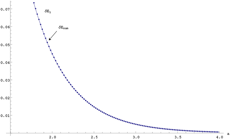
Figure 2. Numerical and first order perturbation results for the splitting in the energy as a function of a for μ = 1 unit in two dimensions.

The same method can also be applied to the one-dimensional case. In the symmetrically placed Dirac delta potentials with equal strengths λ, the exact bound state energies when they are sufficiently far away from each other (when a > 1/λ, there are two bound state energies) can analytically be computed [41]

$\begin{array}{ll}{E}_{\pm }=-{\left(\frac{\lambda }{2}+\frac{1}{2a}W\left(\pm a\lambda e^{-a\lambda }\right)\right)}^2,\hfill & (138)\end{array}$

where W is the Lambert W function [42], which is defined as the solution y(x) of the transcendental equation ye^y = x. From (17), the principal matrix in this case reads

$\begin{array}{ll}{\Phi }_{ij}\left(E\right)=\{\begin{array}{cc}\frac{1}{\lambda }-\frac{1}{2\sqrt{-E}}\hfill & \text{if }i=j\hfill \\ -\frac{1}{2\sqrt{-E}}{e}^{-2a\sqrt{-E}}\hfill & \text{if }i\ne j\hfill \end{array}.\hfill & (139)\end{array}$

Then, the first order perturbation result following the above procedure gives

$\begin{array}{ll}\delta E_1={\lambda }^2{e}^{-a\lambda },\hfill & (140)\end{array}$

where we have used well-known result $E_B=-\frac{{\lambda }^2}{4}$. Then, one can easily find the error between the exact result δE_exact = E₊ − E₋ and the first order perturbation result δE₁ in the splitting of the energy, see the Figure 3.

FIGURE 3

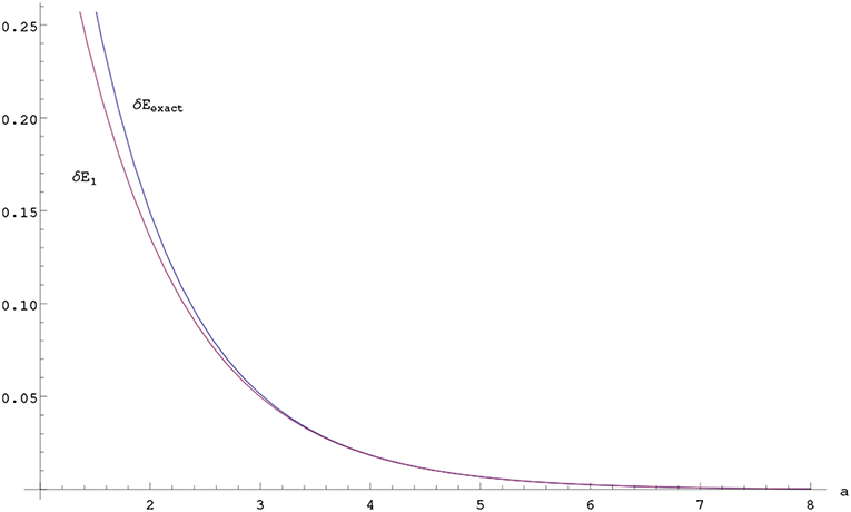
Figure 3. Exact and first order perturbation results for the splitting in the energy as a function of a for λ = 1 unit in one dimension.

The three dimensional case can also be studied in this way and we can similarly solve $det\Phi \left(\nu \right)=\left(\nu -\mu \right)-\pm \frac{1}{2a}{e}^{-2a\nu }$ in terms of the Lambert W function and compare with the first order perturbation result for the splitting in the energy (Figure 4):

FIGURE 4

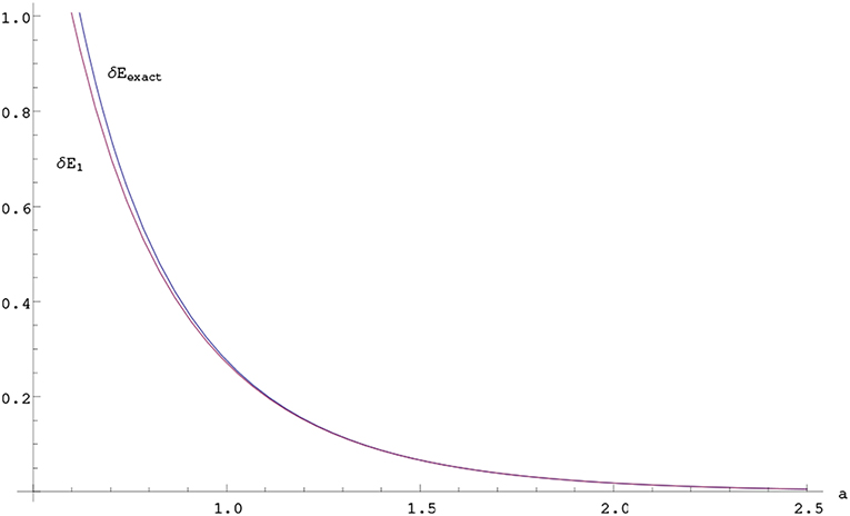
Figure 4. Exact and first order perturbation results for the splitting in the energy as a function of a for μ = 1 unit in three dimensions.

Here we assume that a > 1/2μ in order to guarantee the existence of second bound states.

Let us emphasize that in the usual WKB approach one constructs the wave functions in classically allowed and forbidden regions respectively and use a subtle argument to connect the different regions. In this case, there is really no forbidden region, except the supports of the attractive regions. Indeed right here classically there is no sensible way to define the motion of a particle. Nevertheless, it is possible to find the effect of tunneling for the wave functions from our formalism. It relies on the first order corrections to the eigenstates of the principal operator, notice that an expansion of the eigenstates of the principal operator can be found in the non-degenerate case as

$\begin{array}{ll}{A}^k(E_B^k)=A_0^k(E_B^k)+{\displaystyle \sum _{r\ne k}}\frac{\langle A_0^k(E_B^k),\delta {\Phi }_{kr}(E_B^k)A_0^r(E_B^k)\rangle }{{\omega }_0^k(E_B^k)-{\omega }_0^r(E_B^k)}{A}_0^r(E_B^k).\hfill & (141)\end{array}$

Note that to this order the normalization is not important, moreover we do not need to use a subtle argument about the shift of the eigenvalues since the change of eigenvalue is already second order in the exponentially small quantities, any such correction will be of lower order as we have seen in the shift of energy calculations.

It is well-known that the wave function of the system associated with the bound states can be found from the explicit expression of the resolvent formula. Since the eigenvalues are isolated we can find the projections onto the subspace corresponding to this eigenvalue by the following contour integral (Riesz Integral representation) [5]:

$\begin{array}{ll}{\mathbb{P}}_k=-\frac{1}{2\pi i}{{\displaystyle \oint }}_{C_k}\text{d}zR\left(z\right),\hfill & (142)\end{array}$

where C_k is a small contour enclosing the isolated eigenvalue, say E_k. We note that the free resolvent does not contain any poles on the negative real axis for the Dirac delta potentials supported by points, so all the poles on the negative real axis will come from the poles of inverse principal matrix Φ⁻¹(z). Since the principal matrix is self-adjoint on the real axis, we can apply the spectral theorem. Moreover, its eigenvalues and eigenprojections are holomorphic near the real axis, as emphasized in section 3. Then, we can write the spectral resolution of the inverse principal matrix,

$\begin{array}{ll}{\Phi }_{ij}^{-1}\left(z\right)={\displaystyle \sum _k}\frac{1}{{\omega }^k\left(z\right)}{\mathbb{P}}_k{\left(z\right)}_{ij},\hfill & (143)\end{array}$

where ${\mathbb{P}}_k{\left(z\right)}_{ij}=\overline{A^{ik}\left(z\right)}{A}^{jk}\left(z\right)$, A^ki(z) is the normalized eigenvector corresponding to the eigenvalue ω^k(z). Then, from the residue theorem, we find the square integrable wave function associated with the bound state energy E_k as

$\begin{array}{ll}\begin{array}{c}{\psi }_k\left(\text{x}\right)=\alpha {\displaystyle \sum _{i=1}^N}{R}_0\left(\text{x},{\text{a}}_{\text{i}};E_k\right)A^{ki}\left(E_k\right),\hfill \end{array}\hfill & (144)\end{array}$

where $\alpha ={(-\frac{\partial {\omega }^k}{\partial E}{|}_{E_k})}^{-1/2}$ is the normalization constant. This is actually a general formula for the bound state wave function for the Dirac delta potentials supported by points in ℝⁿ. For n = 2, we have

$\begin{array}{ll}{\psi }_k\left(\text{x}\right)=\frac{\alpha }{2\pi }{\displaystyle \sum _{i=1}^N}{K}_0\left(\sqrt{-E_k}|\text{x}-{\text{a}}_{\text{i}}|\right)A^{ki}\left(E_k\right).\hfill & (145)\end{array}$

Let us recall that the eigenstates for the unperturbed levels are given by unit vectors (103), when we write this into the formula for the wave function (145). As a result, using the first order correction (100) to the eigenstate A^k we find that the change of the wave original wave function in the first order becomes,

$\begin{array}{l}\delta {\psi }_k(x)=\frac{{(4\pi E_B^k)}^{1/2}}{2\pi }{\displaystyle \sum _{l\ne k}}\frac{1}{ln(|E_k^B|/|E_l^B|)}{K}_0(\sqrt{|E_B|}|{\text{a}}_{\text{k}}-{\text{a}}_{\text{l}}|)K_0(\sqrt{|E_k^B|}|\text{x}-{\text{a}}_{\text{l}}|)\hfill \\ ~\sqrt{2}|E_B^k{|}^{1/4}{\displaystyle \sum _{l\ne k}}\frac{1}{ln(|E_k^B|/|E_B^l|)}\frac{e^{-\sqrt{|E_B^k|}|{\text{a}}_{\text{k}}-{\text{a}}_{\text{l}}|}}{\sqrt{|{\text{a}}_{\text{k}}-{\text{a}}_{\text{l}}|}}{K}_0(\sqrt{|E_B^k|}|\text{x}-{\text{a}}_{\text{l}}|),\hfill & (146)\end{array}$

where we use

$\begin{array}{ll}\begin{array}{l}\frac{1}{\left({-\frac{\partial {\omega }_0^k(E)}{\partial E}|}_{E_B^k}\right)}=4\pi |E_B^k|.\hfill \end{array}\hfill & (147)\end{array}$

This form of the wave function clearly shows the tunneling nature of the wave functions. It is now quite straightforward to compute the wave functions in this approximation for all the other cases we consider.

Conclusion

In this paper, we have first reviewed the basic results about some singular interactions, such as the Dirac delta potentials supported by points on flat spaces and hyperbolic manifolds, and delta potentials supported by curves in flat spaces. Moreover, the results in the relativistic extensions of the above-mentioned potentials have been also reviewed which was essentially given in Altunkaynak et al. [13], Erman and Turgut [14], Erman [15], Dogan and Turgut [17], Erman et al. [18], and Kaynak and Turgut[19]. The main result of this paper is to develop some kind of perturbation theory applied to some class of singular potentials in order to find the splitting in the energy due to the tunneling. This was only developed for Dirac delta potentials supported by points in Erman and Turgut [14], here we extend the method for various kind of Dirac delta potentials as well as its relativistic extensions.

It is possible to give some bounds over the error terms if we assume that the errors in perturbation theory can be estimated. Typical perturbative expansions are asymptotic therefore a truncation is needed to get more accurate results, one knows that it gets worse beyond a few terms. The more accurate thing to do is to obtain a Borel summed version but that is beyond the content of the present paper, it will depend very much of the specifics of the model whereas we prefer to give a broader perspective.

The comparison with conventional methods certainly would be very useful, nevertheless at present we do not know how a more conventional approach, such as WKB or instanton calculus can be performed in these singular problems. Since the potentials are localized at points or along the curves, the variation of the potential relative to any wavelength is always much more important. Indeed this unusual behavior changes the problem completely. We need to give a meaning to these potentials first and redevelop the WKB analysis. Our main point here is that in this description of the singular potentials via resolvents, the WKB's reincarnation is given by a perturbative analysis of the eigenvalues of the principal operator for large separations of the supports.

Data Availability

All datasets generated for this study are included in the manuscript and/or the supplementary files.

Author Contributions

All authors listed have made a substantial, direct and intellectual contribution to the work, and approved it for publication.

Conflict of Interest Statement

The authors declare that the research was conducted in the absence of any commercial or financial relationships that could be construed as a potential conflict of interest.

Acknowledgments

The authors would like to thank the editors for their invitation to contribute to the special issue and two referee for his/her valuable comments and suggestions which improve the paper. First author also acknowledges Haydar Uncu for his useful suggestion about the numerical calculations in Mathematica.

References

1. Landau LD, Lifshitz EM. Quantum Mechanics. New York, NY: Pergamon Press (1977).

Google Scholar

2. Das A. Field Theory, A Path Integral Approach. Singapore: World Scientific (1993).

Google Scholar

3. Coleman S. Aspects of Symmetry. Cambridge: Cambridge University Press (1988).

Google Scholar

4. Galindo A, Pascual P. Quantum Mechanics I. Madrid: Springer-Verlag (1990).

Google Scholar

5. Reed M, Simon B. Methods of Modern Mathematical Physics II. New York, NY: Academic Press (1978).

Google Scholar

6. Albeverio S, Gesztesy F, Hoegh-Krohn R, Holden H. Solvable Models in Quantum Mechanics. 2nd ed. Providence, RI: American Mathematical Society (2004).

Google Scholar

7. Albeverio S, Kurasov P. Singular Perturbations of Differential Operators Solvable Schrödinger-type Operators. Cambridge: Cambridge University Press (2000).

Google Scholar

8. Berezin FA, Faddeev LD. A remark on Schrdinger's equation with a singular potential. Soviet Math Dokl. (1961) 2:372–5.

9. Huang K., Quarks, Leptons and Gauge Fields. Singapore: World Scientific (1982).

Google Scholar

10. Jackiw R. in M. A. B. Beg: Memorial Volume. In: Ali A, Hoodbhoy P, editors. Singapore: World Scientific (1991).

Google Scholar

11. Gosdzinsky P, Tarrach R. Learning quantum field theory from elementary quantum mechanics. Am J Phys. (1991) 59:70. doi: 10.1119/1.16691

CrossRef Full Text | Google Scholar

12. Mead LR, Godines J. An analytical example of renormalization in two-dimensional quantum mechanics. Am J Phys. (1991) 59:935. doi: 10.1119/1.16675

CrossRef Full Text | Google Scholar

13. Altunkaynak B, Erman F, Turgut OT. Finitely many Dirac-delta interactions on Riemannian manifolds. J Math Phys. (2006) 47:082110. doi: 10.1063/1.2259581

CrossRef Full Text | Google Scholar

14. Erman F, Turgut OT. Point interactions in two- and three-dimensional Riemannian manifolds. J Phys A Math Theor. (2010) 43:335204. doi: 10.1088/1751-8113/43/33/335204

CrossRef Full Text | Google Scholar

15. Erman F. On the number of bound states of point interactions on hyperbolic manifolds. Int J Geometr Methods Mod Phys. (2017) 14:1. doi: 10.1142/S0219887817500116

CrossRef Full Text | Google Scholar

16. Exner P, Kondej S. Curvature-induced bound states for a δ interaction supported by a curve in ℝ³. Ann Henri Poincarè. (2002) 3:967. doi: 10.1007/s00023-002-8644-3

CrossRef Full Text | Google Scholar

17. Dogan C, Turgut OT. Renormalized interaction of relativistic bosons with delta function potentials, J Math Phys. (2000) 51:082305. doi: 10.1063/1.3456122

CrossRef Full Text

18. Erman F, Gadella M, Uncu H. One-dimensional semirelativistic Hamiltonian with multiple Dirac delta potentials, Phys Rev D. (2017) 95:045004. doi: 10.1103/PhysRevD.95.045004

CrossRef Full Text | Google Scholar

19. Kaynak B, Turgut OT. A Klein Gordon particle captured by embedded curves. Ann Phys. (2012) 327: 2605–16. doi: 10.1016/j.aop.2012.05.008

CrossRef Full Text | Google Scholar

20. Albeverio SA, Exner P, Geyler VA. Geometric phase related to point-interaction transport on a magnetic Lobachevsky plane. Lett Math Phys. (2001) 55:9–16. doi: 10.1023/A:1010943228970

CrossRef Full Text | Google Scholar

21. Brünining J, Geyler VA. Gauge-periodic point perturbations on the Lobachevsky plane, Theor Math Phys. (1999) 119:687–97. doi: 10.1007/BF02557379

CrossRef Full Text | Google Scholar

22. Brüning J, Geyler V, Pankrashkin K. Spectra of self-adjoint extensions and applications to solvable Schrödinger operators. Rev Math Phys. (2008) 20:1–70. doi: 10.1142/S0129055X08003249

CrossRef Full Text | Google Scholar

23. Exner P, Gawlista R, Seba P, Tater M. Point interactions in a strip. Ann Phys. (1996) 252:133–79. doi: 10.1006/aphy.1996.0127

CrossRef Full Text | Google Scholar

24. Rudnick Z, Ueberschär H. Statistics of wave functions for a point scatterer on the torus. Commun Math Phys. (2012) 316:763–82. doi: 10.1007/s00220-012-1556-2

CrossRef Full Text | Google Scholar

25. Exner P, Ichinose T. Geometrically induced spectrum in curved leaky wires. J Phys A Math Gen. (2001) 34:1439. doi: 10.1088/0305-4470/34/7/315

CrossRef Full Text | Google Scholar

26. Appel W. Mathematics for Physics and Physicists. Princeton, NJ: Princeton University Press (2007).

Google Scholar

27. Rajeev SG. Bound states in models of asymptotic freedom. arXiv: hep-th/9902025 (1999).

Google Scholar

28. Lebedev NN. Special Functions and Their Applications. Englewood Cliffs, NJ: Printice Hall (1965).

29. Grigoryan A. Heat Kernel and Analysis on Manifolds. AMS/IP Studies in Advanced Mathematics Vol. 47, Yau S-T, editor. Providence, RI: American Mathematical Society (2009).

Google Scholar

30. Albeverio S, Kurasov P. Pseudo-differential operators with point interactions. Lett Math Phys. (1997) 41:79–92. doi: 10.1023/A:100737012

CrossRef Full Text | Google Scholar

31. Lieb EH, Loss M. Analysis. Graduate Studies in Mathematics. 2nd ed. Providence, RI: American Mathematical Society (2000).

Google Scholar

32. Al-Hashimi MH, Shalaby AM, Wiese U-J. Asymptotic freedom, dimensional transmutation, and an infrared conformal fixed point for the δ-function potential in one-dimensional relativistic quantum mechanics. Phys Rev D. (2014) 89:125023. doi: 10.1103/PhysRevD.89.125023

CrossRef Full Text | Google Scholar

33. Do Carmo MP. Differential Geometry of Curves and Surfaces. Englewood Cliffs, NJ: Prentice Hall (1976).

Google Scholar

34. Gradshteyn IS, Ryzhik IM. Table of Integrals, Series and Products. 7th ed. San Diego, CA: Academic Press (2007).

Google Scholar

35. Rosenblum M, Rovnyak J. Hardy Classes and Operator Theory. New York, NY: Oxford University Press (1985).

Google Scholar

36. Kato T. Perturbation Theory for Linear Operators. Classics in Mathematics, corrected printing of the second edition. Berlin: Springer-Verlag (1995).

Google Scholar

37. Feynman RP. Forces in Molecules, Phys Rev. (1939) 56:340. doi: 10.1103/PhysRev.56.340

CrossRef Full Text | Google Scholar

38. Hellmann H. Einführung in die Quantenchemie. Leipzig: Franz Deuticke (1937). p. 285.

39. Galindo A, Pascual P. Quantum Mechanics II. Madrid: Springer-Verlag (1989).

Google Scholar

40. Bender CM, Orszag SA. Advanced Mathematical Methods for Scientists and Engineers. New York, NY: McGraw-Hill (1999).

Google Scholar

41. Erman F, Gadella M, Uncu H. A singular one-dimensional bound state problem and its degeneracies, Eur Phys J Plus. (2017) 132:352. doi: 10.1140/epjp/i2017-11613-7

CrossRef Full Text | Google Scholar

42. Corless RM, Gonnet GH, Hare DEG, Jeffrey DJ, Knuth DE. On the LambertW function. Adv Comput Math. (1996) 5:329. doi: 10.1007/BF02124750

CrossRef Full Text | Google Scholar