
94% of researchers rate our articles as excellent or good
Learn more about the work of our research integrity team to safeguard the quality of each article we publish.
Find out more
METHODS article
Front. Phys. , 03 May 2019
Sec. Space Physics
Volume 7 - 2019 | https://doi.org/10.3389/fphy.2019.00063
A new approach is presented for interpreting low level Langmuir probe measurements in terms of physical plasma parameters such as density or temperature. Instead of relying on analytic expressions as in most analyses, the method uses regressions combined with a suitably prepared solution library consisting of precomputed probe characteristics for selected plasma parameters. In machine learning language, this amounts to generating a training data set, constructing and training a model, and validating it over a domain of physical parameters of interest. This study aims at establishing the feasibility and limits of the method by using synthetic data sets that can be generated quickly from analytic approximations. The ultimate goal is to use this approach with model training on data sets constructed with detailed kinetic simulations capable of accounting for more physical processes, and more realistic geometry, than are possible with analytic models.
The near-Earth space environment is of strategic importance in commercial, scientific and security endeavors. Space is a dynamic environment in which space-weather events can affect communication, remote sensing, global positioning satellites (GPS), as well as large ground infrastructure such as pipelines and power grids. For those reasons considerable efforts are made to monitor and characterize this harsh and variable environment in order to better understand its behavior and mitigate possible adverse effects. Monitoring and characterizing these conditions relies upon the acquisition of plasma parameters such as the electron and ion densities and temperatures. Because of its relative simplicity, the Langmuir probe is a common instrument used to make such measurements. Langmuir probes are electrodes biased to various voltages with respect to the satellite ground, from which characteristics, that is, current as a function of bias voltage, are measured. These characteristics then constitute low level (L1B in space instrument terminology) data that must then be interpreted in terms of physical parameters (level L2) such as the plasma density, temperature, or spacecraft floating potential. The physics of current collection by Langmuir probes has been studied by many authors over the course of nearly one century [1–7], and the resulting analytic approximations form the basis of probe characteristic interpretation in most laboratory and space experiments. The use of analytic expressions to infer plasma parameters from characteristics is dictated by the need for fast algorithms capable of providing answers in real time. Unfortunately, analytic approximations cannot account for a combination of the many physical processes at play in the lab or in space, such as the effect of a magnetic field, plasma drift, or the proximity to other objects capable of deflecting or intercepting incoming particles. With present computing facilities, an interesting alternative would be to use detailed three-dimensional kinetic simulations capable of accounting for all the relevant physical processes under realistic geometry conditions. Kinetic simulations have been, and continue to be, applied to specific case studies and elucidate selected processes [8–10] but, due to the considerable computational resources and run times that they require, they cannot be used in real-time interpretation of probe measurements. An approach is proposed here to process low level L1B data from probe measurements (current as a function of voltage) into higher level L2 data (density, temperature, floating potential, …) from kinetic simulations. The method consists of constructing a data set of probe characteristics for a given satellite and probe geometry, corresponding to selected plasma parameters. Given a measured characteristic, the corresponding plasma parameters would then be inferred with an adequate multivariate regression from the set of precomputed solutions, or “solution library.” This can be thought of as a specialized interpolation of plasma parameters in the space of probe characteristics. For simplicity in this first feasibility study, all characteristics are calculated analytically in the Orbital Motion Limited (OML) approximation, with the assumption that the results obtained with these synthetic data will bear relevance to those that would be obtained using computer simulations.
In the following we assess the feasibility of using multivariate regression to infer higher level plasma parameters from low level probe characteristics. The method used to construct a synthetic data base is explained, as well as two regression approaches based on kriging and neural networks. Results obtained with these two approaches are then presented. We conclude with a summary of our findings and concluding remarks.
Two regression approaches are considered, both requiring training and validation data sets of varying size. As mentioned in the introduction, it would be prohibitively time consuming to construct such sets from computer simulations because of the large computing resources that would be required. Thus, for the purpose of evaluating the approaches, synthetic data sets are generated using the analytic OML approximation. This approximation is used here for speed and convenience, without any assumption concerning its accuracy.
We assume a drifting Maxwellian velocity distribution
for electrons and ions (α being e and i, respectively), where nα, Tα, and mα are the density, temperature and mass of species α, and k is the Boltzmann constant. The thermal speed of species α is defined as , and the normalized drift speed as xαd = vdα/vthα. For a repulsive potential qαV > 0 where qα is the particle charge and V is the potential with respect to background plasma, the minimum speed far from the probe, at which a particle can reach the probe, is given by . Defining x = vαm/vthα, and making use of conservation of energy and angular momentum of incident particles, it can be shown after some algebra and integrations in velocity space, that in the OML approximation, the current collected by a spherical probe of radius a is given by
if V < 0, and
if V > 0, where a single ion species with unit charge e is assumed, and plasma is assumed to be neutral with ne = ni = n. In actual measurements, a characteristic also depends on other factors such as the strength and direction of a magnetic field, the proximity to other satellite components, solar illumination and associated photoelectron emission. These effects are neglected here for simplicity. The regression problem considered then reduces to an inversion problem whereby a measured characteristic I has to be interpreted in terms of one or several of the physical parameters that it depends on. The first step in our approach consists of constructing data sets, or solution libraries that are representative of ionospheric conditions. This is done by “numerically sampling” the ionosphere with the International Reference Ionosphere (IRI) model [11] over a range of time periods, altitudes, latitudes and longitudes as listed in Table 1, and from there, construct a large set of points in a representative domain of ionospheric plasma parameters. The result is shown in Figure 1 in which a subset of 5, 000 randomly selected points are plotted in the n − T plane. For simplicity and for the purpose of assessing the feasibility of the proposed regression approaches, we assume equal electron and ion temperatures (Te = Ti = T), a pure O+ plasma, and a fixed plasma flow speed vd = 7, 000 m/s. For each (n, T) in the set, a characteristic is calculated using Equations 2 and 3, and parameterized in terms of 25 currents calculated for 25 voltages V uniformly distributed between −5 and +5 V. Characteristics therefore consist of 25-tuples, or vectors = (I1, I2 , …, I25) from which plasma parameters will be inferred. The set of characteristics with associated n and T then constitutes our full data set, or solution library. Models are trained using “training data sets” made of subsets of the solution library, and their skills are assessed by comparing their predictions against known values from validation data sets made of different subsets of the full library. Our models' skill are defined quantitatively as the largest relative error of model predictions as defined in Equation 6 over a given validation data set. Training data sets consist typically of 6–100 entries, while validation data sets consist of approximately 5, 000 randomly selected entries.
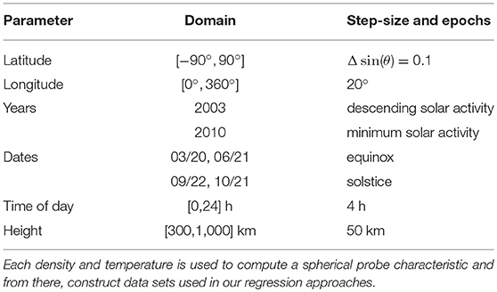
Table 1. Parameters used to define the spatial and temporal ranges for sampling ionospheric densities and temperatures using the IRI model.
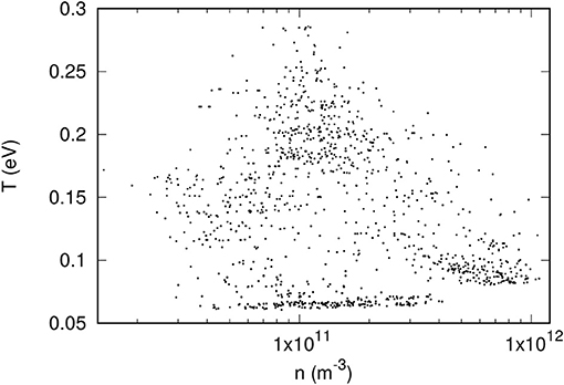
Figure 1. Illustration of the n − T ionospheric-relevant parameter space generated with the IRI model.
Kriging was first introduced in geostatistics to map the distribution of geological formations from limited field samples [12]. The mathematical basis of the approach has later been further developed and applied to a variety of other problems [13–16]. The method has a simple approach which lends itself to providing fast computational speeds. In its complete form, kriging provides models which are statistically unbiased to normal statistical errors in given input data sets. It can be constructed to do collocation at selected data points and relax collocation at others in order to account for “nugget effects,” where uncertainties are known to be larger [17]. In what follows we use a simplified formulation in which the affine terms used to remove bias, and the terms used to account for nugget effects, are not included. The result is pure collocation at selected “pivots,” or points in parameter space, positioned so as to best approximate a given physical variable in a given validation set. Assuming a scalar field p (e.g., density or temperature) to be predicted, from measured characteristics , the modified multivariate kriging model has the form
where Np is the number of pivots used in the model, G is a suitably chosen scalar function of a real variable, are vector characteristics computed at selected pivots (nj, Tj) in parameter space, and aj are fitting coefficients determined by requiring collocation at pivots; that is, by solving for
where yi are known values from the training data set. In these equations, the arguments of G are the norms of the vector differences. The construction and optimization of a model then reduces to selecting:
• a function G which gives the “best” predictions over a given validation data set,
• a number of pivots N, and
• the positions of pivots in parameter space, which minimize the maximum error in the predictions over a given validation data set.
Several functions G have been considered, including G(x) = x, x2, x2ln(x), and x2exp(−x/λ) and the latter has been adopted with λ = 1 for density, and λ = 1.5 for temperature, for empirically giving the best approximations. The choice of a number of pivots N is straightforward, and its effect on a model skill is obvious; model predictions become increasingly accurate with larger values of N. More importantly, the distribution of pivots in parameter space has a direct impact on the accuracy with which model predictions can be made. Pivots must be positioned so as to best capture the connection between characteristics and plasma parameters in the full range considered. The strategy used to determine the optimal pivot positions is described in section 3.1.
The goal is to position Np pivots in a relevant domain in parameter space so that, for a given function G, Equation 4 gives the best approximation of known data values in a given validation data set. In this analysis “best approximation” is determined by the maximum relative error ϵr in the prediction, as defined by
where Nv is the number of entries in the validation data set, and pi is the model prediction given by Equation 4. With this definition, the model can be optimized so as to ensure predictions within a known maximum relative uncertainty ϵr.
The distribution of pivots in the parameter space is done by constructing an unstructured triangular mesh with Nv vertices, enclosing the points in Figure 1, and by successively trying all combinations of Np pivots among the Nv vertices in the mesh. This is illustrated in Figure 2 with a mesh consisting of 70 vertices.
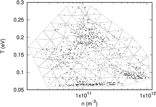
Figure 2. Illustration of a 70 vertex triangular mesh used to find optimal pivot positions in n − T parameter space.
In each combination, the maximum relative prediction error is determined using the validation set, and the distribution of pivots giving the lowest maximum relative error is selected for the model. Considering that pivots are indistinguishable (swapping two pivots produces the same model), the number of combinations Nc is
With several pivots and many mesh points, this number can be quite large. Combined with a large validation set, a direct approach in which all pivot positions are optimized simultaneously might require many hours or days. In such cases, it may be more practical to proceed in steps—first optimizing a few pivots, fixing their positions, and then incrementally adding more until the desired model accuracy is achieved.
Kriging has been applied to construct models to approximate the density n and temperature T in a set of 5000 entries as described in section 2.1. Several numbers of pivots have been considered, using triangular meshes with numbers of nodes ranging from 33 to 70. As expected it is found that smaller meshes generally yield less accurate models. However, model accuracy does not necessarily increase monotonically with the size of the mesh and, for the mesh sizes considered, the changes in accuracy were not significant. For a given mesh however, the model skill always increases with the number of pivots. The results presented here were all obtained with the mesh illustrated in Figure 2, consisting of 70 vertices distributed approximately uniformly in a log(n) - T plot. In both cases, several numbers of pivots have been considered, with direct and incremental optimization. For example, with direct optimization of 5 pivots, model predictions have a maximum relative error of 1.3% for n and 4.3% for T. These errors in turn are 2.0 and 9.3%, respectively, with 3+3 incremental optimization. A loss of model accuracy with the incremental optimization is expected because it does not involve all pivots simultaneously. With multidimensional domains in parameter space and large validation sets, however, the incremental optimization may be the only practical option. The skill of the model constructed for the density with a direct optimization of 5 pivots is shown in Figures 3, 4. In Figure 3, the dashed line shows what is expected for a perfect one-to-one correlation between model and data. In addition to relative errors, Figure 4 also shows the positions of pivots with empty circles. Similarly, Figures 5, 6 show the skill of a model constructed for the temperature using direct optimization of six pivots. The model in this case is less accurate than that for the density, with a maximum relative error of 4.3%. The correlation between model and data temperatures in Figure 5 is noticeably different from that in Figure 3 for the density. While the latter shows apparent random scatter on either side of a perfect correlation, the former seems to follow a thin trajectory with no apparent random scatter, but with structured deviations from the dashed line. Finally, it is worth noting the differences in pivot positions between the two cases. In a practical application of this approach, in which a solution library would be obtained from kinetic simulations, much fewer entries would be computed than are available here with the OML approximation. If more than one physical variable is to be inferred with kriging-based regression, it would be best if pivots optimized for different variables were nearly the same, at least in part. The distribution of pivots in Figures 4, 6, however, suggests otherwise. While some pivots are at nearby positions in the two figures, differences are seen to be appreciable for most of them. The optimization of a model capable of inferring more than one plasma parameter from measured characteristics would therefore likely require more pivots than for a single parameter, as well as a compromise between the inference skill for these different parameters.
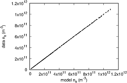
Figure 3. Comparison between model-predicted and actual densities from the validation data set. The model used here was constructed with a direct optimization of five pivots. The dashed line corresponds to a perfect correlation between the two densities.
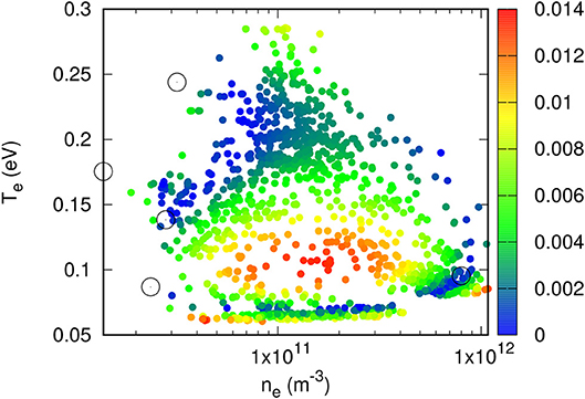
Figure 4. Color plot of relative errors in model-inferred densities in a validation data set consisting of approximately 5, 000 randomly selected points. Circles show the positions of the five directly optimized pivots used to construct the kriging model.
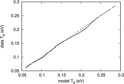
Figure 5. Comparison between model-predicted and actual data temperature values. The model used here was constructed with a direct optimization of six pivots. The dashed line corresponds to a perfect correlation between the two temperatures.
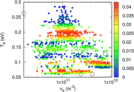
Figure 6. Color plot of relative errors in model-inferred temperatures in a validation data set consisting of approximately 5, 000 randomly selected points. Circles show the positions of the six directly optimized pivots used to construct the kriging model.
Artificial neural networks have been studied extensively in the last several decades. They are derived from cognitive theory in the human brain, where a neural network consists of connections and nodes. In a computational setting, it is the goal of these networks to optimize numerical weights (connections) such that they map independent variables to a specific dependent outcome, or simply perform regression on a given set of data. A schematic of a neural network is shown in Figure 7.
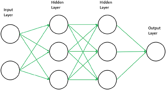
Figure 7. Schematic of a feed forward neural network. Arrows represent the weight values that are optimized during the training of a neural network model and circles represent the nodes.
This type of network is known as feed forward, where the inputs are propagated forward through the network. In practice, each node in the input layer is assigned a numerical value u0, j where 0 stands for the input layer, and j is the node index in that layer. Node values are then transformed and fed to the nodes of the following layer and so on, until reaching the output layer. To be specific, given values ui, j in node j of layer i, node m of the following layer would then be assigned ui+1, m as follows:
where ni is the number of nodes in layer i, wi, j, m are weight factors, bi, j are bias terms, and f is a nonlinear activation function. The activation function is a key component in neural networks for their ability to capture complex dependencies in a data set, and its choice can greatly impact the quality of model predictions. In practice, training the network involves the minimization of a positive cost function that measures the discrepancy between predicted pi and data values yi on a given training data set. The cost function used in this study is
where N is the number of entries in the training data set. In the problem considered here, the input layer contains probe characteristics, which are parameterized in terms of 25 currents for given 25 voltages. The network used to perform the regressions consists of an input layer of 25 nodes, for each component of a 25-tuple current, (I1, I2 , …, I25), two hidden layers of 25 and 13 nodes and a single output node for either the predicted density or temperature. Minimization of the cost function is done through a backpropagation algorithm, such that the discrepancies in the cost function are propagated backwards to each weight [18, 19].
All neural networks utilized in this study were created with TensorFlow [20], and the cost functions were minimized with the Adam algorithm, an improved backpropagation, which has been shown to achieve very high levels of accuracy in many common machine learning problems [21]. The bias terms appearing in Equation 8 are ignored (all set to zero) because they are found to make no significant difference in the outcome, and the activation function f used is the hyperbolic tangent; f(x) = tanh(x) which ranges between −1 and +1. Finally, a simple normalization technique was used to ensure all training input values were bound between −1 and +1, the same range as the hyperbolic tangent function, which is known to aid in the training process for neural networks to avoid saturation of values in certain nodes [18]. However, as a result of this normalization scheme, input characteristics used in the validation of a network could have normalized values beyond −1 or +1, forcing the network to extrapolate outside its training range.
By adopting the same pivots found in section 3.2, both density and temperature models were created with neural networks. However, results were found to be sub-optimal, with maximum relative errors in n and T above 100%. Instead, to indicate the performance of neural networks in this regression problem, training data sets with 20, 50, and 100 characteristics were generated from random density and temperature pairs from our full IRI database.
As expected, increasing the size of the training data set increases the accuracy of the network for predicting plasma parameters. For the smallest models, where only 20 characteristics were used in training, the networks are able to generalize very well considering the system is severely under-determined. The networks were able to train to a maximum relative error in the testing set of 16 and 27% for n and T respectively. At this small training set size, it was clear that the temperature models were comparable to density models in mean relative error as they both obtained below 10% for this metric. However, when training a network for temperature predictions, it was very difficult to find a random set of 20 characteristics such that the maximum relative error was comparable to the results for density.
As the training data sets were increased in size to 50 and 100 entries, maximum relative errors below 10% and mean relative errors of roughly 3% were obtained for both n and T. Figures 8–11 illustrate the skill of the model trained with 100 data entries. The correlation between predicted and known values of the density, and temperature respectively in Figures 8 and 10 is very good, as there is a strong linear trend along the diagonal in both plots, indicating very little deviation from absolute accuracy. Furthermore, Figures 9, 11 display the prediction skill for each point in the testing data set on the n − T plane. Here there is better evidence for the claims surrounding the unreliability in randomly selecting the training data points, which are shown as the black circles. In regions where they are heavily concentrated, the local accuracy of surrounding points is generally very high. Conversely, in regions where training points are more sparse, the accuracy drops. However, in some instances there may be a concentration of training points, and very near to this the prediction skill drops off rapidly. This effect of course cannot be tracked and remedied when the entries for the training data set are selected at random, suggesting that perhaps if points from denser regions could be moved to these areas of reduced accuracy, the skill of the entire network would be increased.
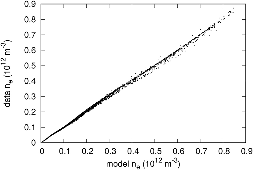
Figure 8. Comparison between model-predicted and actual densities from the validation data set. The neural network used here was trained with 100 randomly selected characteristics. The dashed line corresponds to a perfect correlation between the two densities.
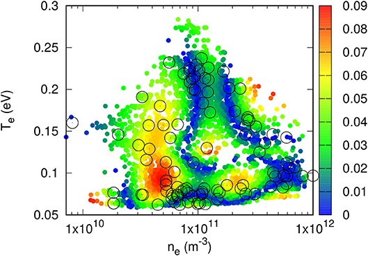
Figure 9. Color plot of relative errors in model-inferred density in a validation data set consisting of approximately 5, 000 randomly selected points. Circles show the positions of the 100 density and temperature pairs corresponding to the randomly selected characteristics.
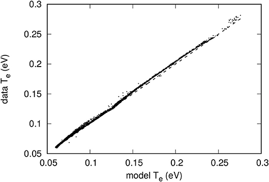
Figure 10. Comparison between model-predicted and actual temperatures from the validation data set. The neural network used here was trained with 100 randomly selected characteristics. The dashed line corresponds to a perfect correlation between the two temperatures.
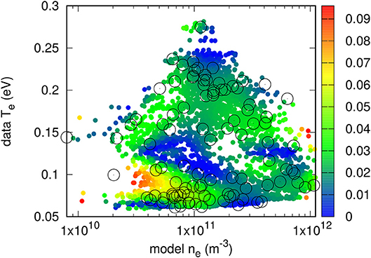
Figure 11. Color plot of relative errors in model-inferred temperature in a validation data set consisting of approximately 5, 000 randomly selected points. Circles show the positions of the 100 density and temperature pairs corresponding to the randomly selected characteristics.
Due to the effects discussed above, the training data sets should be optimized to best represent the entire n − T parameter space. It was clear that random selection was not an optimal method in determining the n − T pairs from the IRI database, as this was found to drastically effect the skill of the models created with 20 and 50 characteristics. Often, a random selection would result in the maximum relative error for the testing data set to remain at very high values (>100%) during training. This could also be a result of the initialization of weights at the beginning of training as this process is also random, furthering the challenge to find the global minimum of the cost function. An approach similar to the pivot selection method with kriging, but in a neural network setting, could be possible and should be explored. This problem was considered, however a stopping condition during the training of a network was difficult to define, as the training procedure can be limited to a number of iterations or an accuracy threshold. With both of these cases, the number of iterations may be too large or a threshold may never be reached, making this approach very volatile to hyper-parameter adjustment, compared to kriging's rather simple analysis on a set of pivots.
The task of obtaining a subset of data, such that its prediction skill is equivalent to that of an optimal data set, is known as instance selection. Computational techniques such as wrapper and filter algorithms have been applied to instance selection problems and were reviewed by Olvera-López et al. [22]. With these algorithms, a more rigorous selection would be made for a small data set compared to a random sampling method. Other future considerations should involve the application of few-shot learning, where a neural network is given a small amount of data and is then tasked with learning the entire nature of the given data [23–26]. Often, this is done in image classification problems, where the network has access to many images that are similar to the new class of image in question and thus uses this pre-trained network to aid in the few-shot learning process. In a regression model proposed by Finn et al. [27], they show that a few-shot approach (10 training examples) provides state-of-the-art results for classification and regression problems. It is important to reiterate that an assumption was made regarding the likeness of the synthetic data used in this study to that of real plasma environments. Without adequately tested and controlled data sets, it cannot be concluded if neural networks will produce the same skill when analyzing kinetically simulated characteristics. A physical model that best characterizes plasma behavior in the Ionosphere should be applied to the neural network approach.
Two regression approaches were presented and applied to infer plasma parameters from Langmuir probe characteristics. One is based on a simplified version of kriging developed and used in geostatistics, and the other uses a neural network as developed for machine learning and artificial intelligence. The goal of this study is to assess the feasibility of using regression techniques to interpret probe characteristics in terms of physical parameters, given a data set, or solution library, consisting of probe characteristics and corresponding plasma parameters. Sets of representative ionospheric plasma parameters at different times and locations were generated using the International Reference Ionosphere (IRI) model, which is a statistical model based on a combination of observations and computer models. For simplicity, in this feasibility study, only the density n and temperature T are considered as independent plasma parameters. For each pair (n, T) a probe characteristic is calculated analytically in the Orbital Motion Limited (OML) approximation. The combination of probe characteristics with corresponding plasma parameters then forms synthetic training and validation data sets used to construct regression models and assess their skills. While approximate, the assumption is that the results obtained with synthetic data are indicative of what to expect with more physically accurate data sets constructed from detailed kinetic simulations or measurements. Model predictions with relative errors below 10% were possible with kriging and neural networks for both plasma density and temperature. Models constructed with kriging made use of pivots positioned optimally in parameter space, so as to minimize the maximum relative error in a given validation data set. With neural networks, the pivot approach was not practical, and accurate models were only possible with sufficiently large (50–100 entries) training data sets. All data sets were created randomly for neural networks, thus requiring further exploration to produce a more sophisticated selection method to test if smaller data sets (20 or less) will provide similar results to those of large sets. Such future work should include instance selection and few-shot learning techniques to improve the quality and relevance of training examples used in neural network models. Owing to the large computing resources and run times required, our results suggest that it should be practical to construct regression models with kriging, because this approach can be used with relatively small training data sets or equivalently, small numbers of pivots. A model based on a neural network, on the other hand, requires larger training sets in order to produce the same level of accuracy. Such an approach may be practical for data sets constructed from accurate and validated measurements provided that sufficiently large (>20) data sets can be constructed. The analysis considered here focused on only two physical parameters n and T, with the assumption that plasma consisted of a single ion species (O+) and that voltages Vi with respect to background plasma were known. In general, electron and ion temperatures may differ, there may be several ion species with different masses and charges, and probe voltages are not known with respect to background plasma but rather with respect to the spacecraft ground. Thus, with Vfl being the spacecraft floating potential, and Vb, i being the probe bias voltages with respect to ground, it follows that
which introduces Vfl as an unknown parameter. Many spacecraft have means of determining the floating potential [28–34]. With an independent measurement of Vfl it would be straightforward to extend the analysis considered here by accounting for the fact that a non-zero floating potential simply changes voltages by an additive constant. Another possibility would be to use the regression techniques to infer Vfl directly from the characteristics. The inclusion of this unknown, as well as others such as the ion temperature, mass and charge composition, should also be considered in a generalized regression problem, and those will be accounted for in future studies. In closing, we reiterate that simplifications have been made in this first assessment of the proposed methodology. In particular, synthetic data was used in lieu of kinetically computed characteristics, and noise was omitted for simplicity. Nonetheless, we conclude that regression with kriging, and possibly neural networks, is of interest for better interpreting particle sensor measurements and is worth pursuing.
JC was responsible for all analysis pertaining to the machine learning aspect of the article. RM was responsible for all analysis pertaining to the Kriging aspect of the article. Both RM and JC were involved in drafting the article where each author focused on their respective analysis portion and shared the workload for the other sections.
The authors declare that the research was conducted in the absence of any commercial or financial relationships that could be construed as a potential conflict of interest.
This work was supported by the Natural Sciences and Engineering Research Council of Canada.
1. Mott-Smith HM, Langmuir I. The theory of collectors in gaseous discharges. Phys Rev. (1926) 28:727.
2. Laframboise J, Parker L. Probe design for orbit-limited current collection. Phys Fluids. (1973) 16:629–36.
3. Godyak V, Piejak R, Alexandrovich B. Probe diagnostics of non-Maxwellian plasmas. J Appl Phys. (1993) 73:3657–63.
4. Sanmartın J, Estes RD. The orbital-motion-limited regime of cylindrical Langmuir probes. Phys Plasmas. (1999) 6:395–405.
5. Allen J, Annaratone B, De Angelis U. On the orbital motion limited theory for a small body at floating potential in a Maxwellian plasma. J Plasma Phys. (2000) 63:299–309. doi: 10.1017/S0022377800008345
6. Lampe M. Limits of validity for orbital-motion-limited theory for a small floating collector. J Plasma Phys. (2001) 65:171–80. doi: 10.1017/S0022377801001027
7. Delzanno GL, Tang XZ. Comparison of dust charging between orbital-motion-limited theory and particle-in-cell simulations. Phys Plasmas. (2015) 22:113703. doi: 10.1063/1.4935697
8. Imtiaz N, Marchand R, Lebreton JP. Modeling of current characteristics of segmented Langmuir probe on DEMETER. Phys Plasmas. (2013) 20:052903. doi: 10.1063/1.4804336
9. Rehman Su, Fisher LE, Lynch KA, Marchand R. Kinetic modeling of Langmuir probe characteristics in a laboratory plasma near a conducting body. Phys Plasmas. (2017) 24:012901. doi: 10.1063/1.4972879
10. Marchand R. Ionospheric langmuir probe electron temperature asymmetry and magnetic field connectivity. IEEE Trans Plasma Sci. (2017) 45:1923–6. doi: 10.1109/TPS.2016.2619668
11. Bilitza D, Altadill D, Zhang Y, Mertens C, Truhlik V, Richards P, et al. The international reference ionosphere 2012–a model of international collaboration. J Space Weather Space Clim. (2014) 4:A07. doi: 10.1051/swsc/2014004
12. Krige DG. A statistical approach to some basic mine valuation problems on the Witwatersrand. J South Afr Inst Min Metallurgy. (1951) 52:119–39.
13. Wackernagel H. Multivariate geostatistics: an introduction with applications. In: International Journal of Rock Mechanics and Mining Sciences and Geomechanics Abstracts. Vol. 33, Berlin Heidelberg: Springer (1996). p. 363A.
14. Dai K, Liu G, Lim K, Gu Y. Comparison between the radial point interpolation and the Kriging interpolation used in meshfree methods. Comput Mech. (2003) 32:60–70.
15. Hengl T, Heuvelink GB, Rossiter DG. About regression-kriging: from equations to case studies. Comput. Geosci. (2007) 33:1301–15.
16. Stein ML. Interpolation of Spatial Data: Some Theory for Kriging. New York, NY: Springer Science & Business Media (2012).
18. Goodfellow I, Bengio Y, Courville A. Deep Learning. MIT Press (2016). Available online at: http://www.deeplearningbook.org
19. Nielsen MA. Neural Networks and Deep Learning. Determination Press (2015). Available online at: http://www.neuralnetworksanddeeplearning.com
20. Abadi M, Barham P, Chen J, Chen Z, Davis A, Dean J, et al. Tensorflow: a system for large-scale machine learning. In: Proceedings of the 12th USENIX Symposium on Operating Systems Design and Implementation. Vol. 16, Savannah, GA (2016). p. 265–83.
21. Kingma DP, Ba J. Adam: a method for stochastic optimization. arXiv preprint arXiv:14126980. (2014).
22. Olvera-López JA, Carrasco-Ochoa JA, Martínez-Trinidad JF, Kittler J. A review of instance selection methods. Artificial Intelligence Review. 2010;34:133–143.
23. Snell J, Swersky K, Zemel R. Prototypical networks for few-shot learning. In: Advances in Neural Information Processing Systems. Long Beach, CA (2017). p. 4077–87.
24. Vinyals O, Blundell C, Lillicrap T, Wierstra D, et al. Matching networks for one shot learning. In: 30th Conference on Neural Information Processing Systems (NIPS). Barcelona (2016). p. 3630–38.
25. Fei-Fei L, Fergus R, Perona P. One-shot learning of object categories. IEEE Trans Pattern Anal Mach Intel. (2006) 28:594–611.
26. Fe-Fei L, Fergus R, Perona P. A bayesian approach to unsupervised one-shot learning of object categories. In: Computer Vision, 2003. Proceedings. Ninth IEEE International Conference on. Washington, DC: IEEE. (2003). p. 1134–41.
27. Finn C, Abbeel P, Levine S. Model-agnostic meta-learning for fast adaptation of deep networks. arXiv preprint arXiv:170303400. (2017).
28. Montgomery MD, Asbridge J, Bame S, Hones E. Low-energy electron measurements and spacecraft potential: vela 5 and Vela 6. In: Photon and Particle Interactions With Surfaces in Space. Dordrecht; Boston, MA: Springer (1973). p. 247–61.
29. Decreau P, Etcheto J, Knott K, Pedersen A, Wrenn G, Young D. Multi-experiment determination of plasma density and temperature. Space Sci Rev. (1978) 22:633–45.
30. Pedersen A, Cattell C, Fälthammar CG, Formisano V, Lindqvist PA, Mozer F, et al. Quasistatic electric field measurements with spherical double probes on the GEOS and ISEE satellites. Space Sci Rev. (1984) 37:269–312.
31. Hershkowitz N, Cho M. Measurement of plasma potential using collecting and emitting probes. J Vac Sci Technol. (1988) 6:2054–9.
32. Schmidt R, Arends H, Pedersen A, Rüdenauer F, Fehringer M, Narheim B, et al. Results from active spacecraft potential control on the Geotail spacecraft. J Geophys Res. (1995) 100:17253–9.
33. Riedler W, Torkar K, Rüdenauer F, Fehringer M, Pedersen A, Schmidt R, et al. Active spacecraft potential control. In: The Cluster and Phoenix Missions. Dordrecht: Springer (1997). p. 271–302.
Keywords: plasma parameters, langmuir probe measurements, regression, neural network, kriging
Citation: Chalaturnyk J and Marchand R (2019) A First Assessment of a Regression-Based Interpretation of Langmuir Probe Measurements. Front. Phys. 7:63. doi: 10.3389/fphy.2019.00063
Received: 05 February 2019; Accepted: 09 April 2019;
Published: 03 May 2019.
Edited by:
Rudolf A. Treumann, Ludwig Maximilian University of Munich, GermanyReviewed by:
Haiyang Fu, Fudan University, ChinaCopyright © 2019 Chalaturnyk and Marchand. This is an open-access article distributed under the terms of the Creative Commons Attribution License (CC BY). The use, distribution or reproduction in other forums is permitted, provided the original author(s) and the copyright owner(s) are credited and that the original publication in this journal is cited, in accordance with accepted academic practice. No use, distribution or reproduction is permitted which does not comply with these terms.
*Correspondence: Richard Marchand, cmljaGFyZC5tYXJjaGFuZEB1YWxiZXJ0YS5jYQ==
Disclaimer: All claims expressed in this article are solely those of the authors and do not necessarily represent those of their affiliated organizations, or those of the publisher, the editors and the reviewers. Any product that may be evaluated in this article or claim that may be made by its manufacturer is not guaranteed or endorsed by the publisher.
Research integrity at Frontiers

Learn more about the work of our research integrity team to safeguard the quality of each article we publish.