Vacuum Energy for Generalized Dirac Combs at T = 0

The quantum vacuum energy for a hybrid comb of Dirac δ-δ′ potentials is computed by using the energy of the single δ-δ′ potential over the real line that makes up the comb. The zeta function of a comb periodic potential is the continuous sum of zeta functions over the dual primitive cell of Bloch quasi-momenta. The result obtained for the quantum vacuum energy is non-perturbative in the sense that the energy function is not analytical for small couplings.

1. Introduction

In this paper we analyse a generalization of the Kronig-Penney model [1] in which the periodic point potential considered is a combination of the Dirac δ-potential and its first derivative, i.e., the δ-δ′ potential (see ref. [2]). Note that the Kronig-Penney model is an example of a one dimensional exactly solvable periodic potential, widely used in Solid State Physics to describe electrons moving in an infinite periodic array of rectangular potential barriers. The δ-δ′ potential has been a focus of attention over the last few years [3–7], but the δ-δ′ comb as a classical background in interaction with a scalar quantum field has not been considered.

The main goal of this work is to compute the quantum vacuum energy of a scalar field propagating in a (1+1)-dimensional spacetime in interaction with the background of a generalized Dirac comb composed of δ-δ′ potentials (see [2–4]). Interpreting the scalar field as electrons (disregarding spin) we would get a (non-additive) contribution to the internal energy of the lattice. In a periodic structure it is possible to calculate the quantum vacuum energy per unit cell, which gives a contribution to the internal pressure of the lattice. In addition, it is possible to interpret the quantum scalar field as phonons of the lattice. In such a case we would obtain the phonon contribution to the internal pressure of the lattice when computing the quantum vacuum energy per unit cell. However, since the (1+1)-dimensional quantum field theory is a highly simplified theoretical model we will not go into more detail about the interpretation.

Specifically, we study the one dimensional periodic Hamiltonian

$\begin{array}{ll}{H}=-\frac{{\hslash }^2}{2m}\frac{d2}{dx2}+V(x)\text{ where }V(x)={\displaystyle \sum _{n\in \mathbb{Z}}}\mu \delta (x-nd)+2\lambda {\delta }^{\prime }(x-nd),& (1)\end{array}$

with couplings μ, λ ∈ ℝ, and lattice spacing d > 0. We will work with dimensionless quantities defined as

$\begin{array}{ll}y=\frac{mc}{\hslash }x,a=\frac{mc}{\hslash }d,w_0=\frac{1}{\hslash c}\mu ,w_1=\frac{m}{{\hslash }^2}\lambda ,& (2)\end{array}$

so that [y, a, w₀, w₁] = 1. In that way, the dimensionless time independent Schrödinger equation for the one-particle states of a quantum scalar field is

$\begin{array}{l}\left(-\frac{\partial 2}{\partial y2}+V(y)\right)\varphi (y)=k^2\varphi (y),\\ V(y)={\displaystyle \sum _{n\in \mathbb{Z}}}{w}_0\delta (y-na)+2w_1{\delta }^{\prime }(y-na).& (3)\end{array}$

Its solutions enables us to determine the energy levels and energy bands of the crystal. Following ref. [8] the general form of the band equation in terms of scattering coefficients (t, r_R, r_L) for the compact supported potential from which the comb is built is

$\begin{array}{ll}\text{cos}(qa)=\frac{e^{iak}(t{(k)}^2-r_R(k)r_L(k))+e^{-iak}}{2t(k)},& (4)\end{array}$

being q the quasi-momentum. This equation relates the quasi-momenta q ∈ [−π/a, π/a] in the first Brillouin zone and the wave-vector k. The quasi-momentum determines the Bloch periodicity for a given wave function on the lattice:

$\begin{array}{ll}\varphi (y+a)=e^{iqa}\varphi (y).& (5)\end{array}$

Since the cosine of the left hand side in (4) is a bounded function, the energy spectrum of the system is organized into allowed/forbidden energy bands/gaps. As a particular case, when the scattering data for a Dirac-δ potential V = w₀ δ (x) on the line [9]

$\begin{array}{ll}{t}_{\delta }(k)=\frac{2ik}{2ik-w_0},r_{\delta }(k)=\frac{w_0}{2ik-w_0}& (6)\end{array}$

are plugged into equation (4) we obtain

$\begin{array}{ll}cos(qa)=cos(ka)+\frac{w_0}{2k}sin(ka)& (7)\end{array}$

which is the well known band equation for the Kronig-Penney model [1].

The general secular equation (4) will enable us to calculate the vacuum energy of the crystal. The vacuum energy per unit cell (in the interval [0, a]) is computed by spatially integrating the expectation value of the 00-component of the energy-momentum tensor T_μν:

$\begin{array}{ll}{E}_0={{{\displaystyle \int }}^{}}_0^{a}dy\langle 0\left|T_{00}\right|0\rangle & (8)\end{array}$

The non regularized infinite quantum vacuum energy can be represented as well as the summation over modes of the spectrum corresponding to the one-particle states of the field theory.

$\begin{array}{ll}{E}_0={{{\displaystyle \int }}^{}}_0^{a}dy\langle 0\left|T_{00}\right|0\rangle ={\displaystyle {{\displaystyle \sum }}^{}_n}{k}_n& (9)\end{array}$

being $\left\{{\omega }_n^2=k_n\right\}$ the eigenvalues characterizing the one-particle states of the quantum field theory given by equation (4). The ultraviolet divergences that appear naturally in this expression must be subtracted taking into account the self-energy of the individual potential that makes up the comb and the fluctuations of the field in the chosen background. The calculation of 〈0| T₀₀ |0〉 provides the energy density per unit length within a unit cell. This of course contains much more information than just the total energy contained in a unit cell. Nevertheless, the calculation using Green functions will not be addressed in this paper for most general combs. On the other hand we can compute E₀ using spectral zeta functions [10] to skip the intermediate calculation of 〈0| T₀₀ |0〉 0 for which the exact Green function of the quantum field on the crystal is needed. When using the zeta function approach the infinite contributions are subtracted using the regularized expression for the quantum vacuum energy:

$\begin{array}{ll}{E}_0(s)={\displaystyle \sum _n}{k}_n^{-s}.& (10)\end{array}$

This expression is nothing but the spectral zeta function associated to the Schödinger operator defined in equation (3). In order to subtract the divergences one has to perform the analytic continuation of equation (10) for s to the whole complex plane, and then subtract the contribution of the pole at s = −1. A detailed explanation of how to proceed in most general cases is explained in refs. [10–12].

The structure of the present paper is the following. In section 2 we reproduce some basic results on spectral zeta functions that are needed throughout the paper. The section 3 provides a way to re-interpret a general comb formed by superposition of identical potentials with compact support centered at the lattice points, as a 1-parameter family of pistons mimicked by quasi-periodic boundary conditions using the formalism to characterise selfadjoint extensions developed in ref. [13]. Afterwards in section 4 and subsection 5.1, we will use the results from refs. [13, 14] to give a general formula for the finite quantum vacuum energy general comb formed by superposition of identical potentials with compact support. The subtraction of infinites follows from ref. [13]. The rest of section 5 is dedicated to the numerical results for the particular example of the δ-δ′ comb, and the non-perturbative character inherent to the quantum vacuum energy of this particular example. Finally in section 6 we explain the conclusions of our paper.

2. Some Basics Formulas on Spectral Zeta Functions

In general, given an arbitrary potential with small¹ support and its associated comb, the secular equation (4) can not be solved. Nevertheless, the summation over eigenvalues in (10) can be rewritten down using the residue theorem. In this section we explain the method to replace the summation over eigenvalues in equation (10) by a complex contour integral involving the logarithmic derivative of the function that defines the secular equation (4).

Let Ĥ be an elliptic non-negative selfadjoint, second order differential operator and f_Ĥ(z) an holomorphic function on ℂ such that

$\begin{array}{l}i){\displaystyle \underset{z\to 0}{lim}}{f}_{Ĥ}(z)\ne 0,\infty .\\ ii)\mathrm{\text{If we define}}\\ Z(f_{Ĥ})\equiv \left\{k_n\in ℝ/f_{Ĥ}(k_n)=0\right\}\\ \tilde{\sigma }(Ĥ)\equiv \left\{{\lambda }_n\in {ℝ}^{+}/{\lambda }_n\mathrm{\text{is eigenvalue}}\right\},\\ \mathrm{\text{then}}\forall k_n\in Z(f_{Ĥ}),k_n^2={\lambda }_n\in \tilde{\sigma }(Ĥ).\mathrm{\text{The multiplicity of}}{k}_n\mathrm{\text{is the}}\\ \mathrm{\text{degeneracy of}}{\lambda }_n.\end{array}$

The formal definition of the spectral zeta function associated to Ĥ is

$\begin{array}{ll}{\zeta }_{Ĥ}(s)={\displaystyle \sum _{\tilde{\sigma }(Ĥ)}}{\lambda }_n^{-s}\text{ for Re(s)}>\mathrm{\text{ certain positive real number}}.& (11)\end{array}$

Taking into account that the function

$\begin{array}{ll}\frac{d}{dz}log\left(f_{Ĥ}(z)\right)& (12)\end{array}$

has poles at Z(f_Ĥ) and that the residue coincides with the multiplicity of the corresponding zero, the summation over λ_n is equivalent to the summation over the zeroes of f_Ĥ(z) and therefore can be written as

$\begin{array}{ll}{\displaystyle \sum _{\tilde{\sigma }(Ĥ)}}\left\{\dots \right\}={\displaystyle \sum _{Z(f_{Ĥ})}}\left\{\dots \right\}={\oint }_{C}dz\frac{d}{dz}log\left(f_{Ĥ}(z)\right)\left\{\dots \right\}& (13)\end{array}$

where C is a contour that encloses all the zeroes contained in Z(f_Ĥ). Since Ĥ is an elliptic non-negative selfadjoint, second order differential operator we can ensure Z(f_Ĥ) ⊂ ℝ. Hence we can choose C to be the semicircle in the complex plane [−iR, iR] ∪ {z ∈ ℂ/|z| = R, andarg(z) ∈ [−π, π]} and then deform the contour taking the limit R → ∞. After the limit is done, and with the properties assumed for f_Ĥ(z) we obtain an expression for the spectral zeta function that admits analytical continuation to the whole complex plane:

$\begin{array}{ll}{\zeta }_{Ĥ}(s)=\frac{sin(\pi s)}{\pi }{\displaystyle {\int }_0^{\infty }}dk{k}^{-2s}{\partial }_{k}log\left[f_{Ĥ}(ik)\right].& (14)\end{array}$

In this representation the information about the poles of ζ_Ĥ(s) and the values at s ∈ ℤ is contained in

$\begin{array}{ll}\frac{sin(\pi s)}{\pi }{\displaystyle {\int }_1^{\infty }}dk{k}^{-2s}{\partial }_{k}log\left[f_{Ĥ}(ik)\right].& (15)\end{array}$

Hence it all reduces to study (15) in order to obtain the pole structure (Res) and ζ_Ĥ(s ∈ ℤ). In subsection 3.2 of ref. [14] it can be seen an example where all the calculations can be performed analytically.

3. The Comb as a Piston

In order to perform the calculation of the quantum vacuum energy per unit cell for the comb, it is of great interest to re-interpret the corresponding quantum system as a one-parameter family of hamiltonians defined over the finite interval, by using general quantum boundary conditions in the formalism described in refs. [13, 15]. Bloch's theorem ensures that knowing the wave functions on a primitive cell is equivalent to the knowledge of the wave function in the whole lattice. Hence, if the origin of the real line is chosen in a way that it is coincident with one of the lattice potential centers, then it is enough to study the quantum mechanical system characterized by the quantum hamiltonian

$\begin{array}{ll}H=-\frac{d2}{dx2}+w_0\delta (x)+2w_1{\delta }^{\prime }(x),& (16)\end{array}$

defined over the closed interval [−a/2, a/2], being a the lattice spacing. Since the hamiltonian in (16) is not essentially selfadjoint when is defined over the square integrable functions over the closed interval [−a/2, a/2] we need to impose boundary conditions at x = ±a/2 over the boundary values {ψ(±a/2), ψ′(±a/2)}. If in addition such boundary condition ensures that the domain of the corresponding selfadjoint extension is a set of wave functions that satisfy Bloch's semi-periodicity condition², then we can understand the comb as a 1-parameter family of selfadjoint extensions where the parameter is to be interpreted as the quasi-momentum. Below we construct the family of selfadjoint extensions that model the comb.

To start with, let us study the δ-δ′ potential sitting at x = 0 and confined in the interval [-a/2, a/2]. The hamiltonian of the system is given by (16) and its domain (the space of quantum states) in general would be characterized by the general boundary condition

$\begin{array}{ll}\left(\begin{array}{c}\psi \left(-a/2\right)+i{\psi }^{\prime }\left(-a/2\right)\\ \psi \left(a/2\right)-i{\psi }^{\prime }\left(a/2\right)\end{array}\right)=U\left(\begin{array}{c}\psi \left(-a/2\right)-i{\psi }^{\prime }\left(-a/2\right)\\ \psi \left(a/2\right)+i{\psi }^{\prime }\left(a/2\right)\end{array}\right),& (17)\end{array}$

where U ∈ SU(2). In general any U ∈ SU(2) makes (16) selfadjoint in the interval [−a/2, a/2]. Nevertheless, we are focused on mimicking with (17) Bloch's semi-periodicity condition:

$\begin{array}{l}\psi (a/2)=e^{iqa}\psi (-a/2)\\ {\psi }^{\prime }(a/2)=e^{iqa}{\psi }^{\prime }(-a/2).& (18)\end{array}$

It is straightforward to see that the U that gives rise to (18) is given by

$\begin{array}{ll}{U}_B=\left(\begin{array}{cc}0& e^{i\theta }\\ e^{-i\theta }& 0\end{array}\right).& (19)\end{array}$

Plugging (19) in (17) one gets

$\begin{array}{l}\psi (a/2)+i{\psi }^{\prime }(a/2)=e^{-i\theta }\left[\psi (-a/2)+i{\psi }^{\prime }(-a/2)\right]\\ \psi (a/2)-i{\psi }^{\prime }(a/2)=e^{-i\theta }\left[\psi (-a/2)-i{\psi }^{\prime }(-a/2)\right].& (20)\end{array}$

Adding and subtracting both expressions we obtain

$\begin{array}{l}\psi (a/2)=e^{-i\theta }\psi (-a/2)\end{array}$

$\begin{array}{ll}{\psi }^{\prime }(a/2)=e^{-i\theta }{\psi }^{\prime }(-a/2),& (21)\end{array}$

and making θ = −qa, we obtain the equations (18). Hence, the selfadjoint extension that gives Bloch's condition is given by

$\begin{array}{ll}{U}_B=\left(\begin{array}{cc}0& e^{-iqa}\\ e^{iqa}& 0\end{array}\right).& (22)\end{array}$

In addition let us remember that the matching conditions that define the potential $V=w_0\delta (x)+2w_1{\delta }^{\prime }(x)$ are given by (see ref. [2])

$\begin{array}{l}\left(\begin{array}{c}\psi \left(0^{+}\right)\\ {\psi }^{\prime }\left(0^{+}\right)\end{array}\right)=\left(\begin{array}{cc}\alpha & 0\\ \beta & 1/\alpha \end{array}\right)\left(\begin{array}{c}\psi \left(0^{-}\right)\\ {\psi }^{\prime }\left(0^{-}\right)\end{array}\right)\alpha =\frac{1+w_1}{1-w_1},\\ \beta =\frac{w_0}{1-w_1^2}.& (23)\end{array}$

When we solve the equation:

$\begin{array}{ll}-\frac{d2}{dx2}\psi (x)=k^2\psi (x),& (24)\end{array}$

with the matching conditions (23) and the boundary condition (17) with U = U_B given by (22) we can rearrange everything to write down the secular equation and the general solution in terms of the scattering data for the δ-δ′ potential over the real line as was done in ref. [8]. This approach enables to interpret the δ-δ′ comb as a one-parameter family of quantum pistons by reinterpreting the primitive cell of the comb in the following way:

1. The middle piston membrane is represented by the δ-δ′ potential placed at x = 0. To ensure that the lattice quantum fields satisfy the matching conditions (23) we can assume the ansatz for the one-particle states wave functions in [−a/2, a/2] is given by a linear combination of the two linear independent scattering states determined by the scattering amplitudes of the δ-δ′ potential (see refs. [2–4])

$\begin{array}{l}t=\frac{-2k(w_1^2-1)}{2k(w_1^2+1)+i{w}_0},r_R=\frac{-4k{w}_1-i{w}_0}{2k(w_1^2+1)+i{w}_0},\\ r_L=\frac{4k{w}_1-i{w}_0}{2k(w_1^2+1)+i{w}_0}.& (25)\end{array}$

From this amplitudes the determinant of the scattering matrix reads

$\begin{array}{ll}\Rightarrow \mathrm{\text{det }}{S}_{\delta {\delta }^{\prime }}=t^2-r_R{r}_L=\frac{2k(w_1^2+1)-i{w}_0}{2k(w_1^2+1)+i{w}_0}.& (26)\end{array}$

2. The endpoints of the primitive cell correspond to the external walls of the piston placed at x = ±a/2, and the quantum field satisfies the one-parameter family of quantum boundary conditions depending on the parameter θ = −qa, which is the quasi-momentum, given by the unitary matrix U_B in (19).

The spectral function for U = U_B written in terms of the scattering data (t, r_R, r_L) and the quasi-momentum q is (see formula 34 in ref. [8])

$\begin{array}{ll}h(k)=4k\left[2tcos(qa)-e^{-ika}-e^{ika}(t^2-r_R{r}_L)\right].& (27)\end{array}$

The band structure of this comb is given by those k_j such that h(k_j) = 0. In general the solutions {k₀, k₁, …, k_n, …} are functions of q ∈ [−π/a, π/a], so $k_j{(q)}^2$ is an energy band when we let q take its continuum values in [−π/a, π/a]. In order to use zeta function regularization we need to remove in (27) the 4k global factor to get the “good” spectral function according to section 2 (see refs. [10, 14]). Hence the spectral function to be used in our zeta function regularization approach is given by

$\begin{array}{ll}{f}_q(k)=2t\left[cos(qa)-\frac{1}{2t}(e^{-ika}+e^{ika}(t^2-r_R{r}_L))\right].& (28)\end{array}$

In (27) and (28), t, r_R, r_L are the scattering data for the compact supported potential from which the comb is built up on the real line. In addition it is trivial to see that

$\begin{array}{ll}{f}_q(k)=0\to cos(qa)=\frac{1}{2t}\left[e^{-ika}+e^{ika}(t^2-r_R{r}_L)\right],& (29)\end{array}$

which is the usual form for the band equation written in standard text books such as [16], and generalized in [8]. Note that because $t^2-r_R{r}_L$ is the determinant of the unitary scattering matrix, then $t{(0)}^2-r_R(0)r_L(0)\ne 0$. Hence, in general we can work under the assumption that

$\begin{array}{ll}{\displaystyle \underset{k\to 0}{lim}}{f}_q(k)\ne 0,\infty .& (30)\end{array}$

REMARK

It is of note that all the formulas presented in this section, specially (28) is valid for any comb built from repetition of potentials with compact support smaller than the lattice spacing. All that is needed are the scattering amplitudes for a single potential of compact support over the real line, to obtain the corresponding spectral function that characterises the band structure of the corresponding comb.

4. Spectral Zeta Function for the Crystal

Following the interpretation of the comb as a 1-parameter family of selfadjoint extensions given in the previous section we rethink the band spectrum in the following way

1. For a fixed value of q ∈ [−π/a, π/a], f_q(k) = 0 with f_q(k) given by (28), gives a discrete set of values of k in one-to-one correspondence with ℕ.

2. If we let q take values from −π/a to π/a and put together all the discrete spectra from the previous item, then we will obtain all the allowed energy bands.

Hence in order to perform the calculation of the quantum vacuum energy for a massless scalar field we can write down the spectral zeta function that corresponds to the Schrödinger Hamiltonian of the comb

$\begin{array}{ll}{\displaystyle \sum _{bands}}{\displaystyle {\int }_{\sqrt{{ϵ}_{min}^{(n)}}}^{\sqrt{{ϵ}_{max}^{(n)}}}}dk{k}^{-2s}={\displaystyle {\int }_{-\pi /a}^{\pi /a}}\frac{dqa}{2\pi }\frac{sin(\pi s)}{\pi }{\displaystyle {\int }_0^{\infty }}dk{k}^{-2s}{\partial }_{k}log{f}_q(ik).& (31)\end{array}$

In this way we can write in general the spectral zeta function for the comb as

$\begin{array}{ll}{\zeta }_C(s)=\frac{a}{2\pi }{\displaystyle {\int }_{-\pi /a}^{\pi /a}}dq\frac{sin(\pi s)}{\pi }{\displaystyle {\int }_0^{\infty }}dk{k}^{-2s}{\partial }_{k}log{f}_q(ik).& (32)\end{array}$

Since the integration in q runs over a finite interval, and q enters as a parameter of the selfadjoint extension associated to the unitary operator U_B in (22), all the infinite contributions of the quantum vacuum energy are enclosed in the zeta function for a δ-δ′ potential placed at x = 0 confined between two plates placed at x = ±a/2, i. e.

$\begin{array}{ll}{\zeta }_q(s)=\frac{sin(\pi s)}{\pi }{\displaystyle {\int }_0^{\infty }}dk{k}^{-2s}{\partial }_{k}log{f}_q(ik).& (33)\end{array}$

As a result of the formulas for the spectral zeta function it is easy to conclude that the finite quantum vacuum energy for the comb, $E_{\text{comb}}^{fin}$, can be obtained from the finite quantum vacuum energy $E_0^{fin}(q)$ for the quantum scalar field confined between two plates placed at x = ±a/2 represented by the boundary condition associated to (22), and under the influence of a δ-δ′ potential placed at x = 0:

$\begin{array}{ll}{E}_{\text{comb}}^{fin}=\frac{a}{2\pi }{\displaystyle {\int }_{-\pi /a}^{\pi /a}}dq{E}_0^{fin}(q).& (34)\end{array}$

Hence our problem reduces to compute $E_0^{fin}(q)$.

5. The Finite Quantum Vacuum Energy at Zero Temperature for Generalized Dirac Combs

5.1. General Formulas

From this point we will use formula 2.26 in ref. [13] to obtain $E_0^{fin}(q)$. In ref. [13] there was no point potential between plates, so the final result arising there did not depend on the reference length L₀ used to subtract the infinite parts. In our case the existence of a potential with compact support between plates forces to take the limit L₀ → ∞. Physically this limit means that what we subtract is the quantum vacuum energy of the potential with compact support on the whole real line. With these assumptions and changing the length L in ref. [13] by our lattice spacing a we can write

$\begin{array}{l}{E}_0^{fin}(q)={\displaystyle \underset{a_0\to \infty }{lim}}\frac{-a_0}{2\pi (a-a_0)}\times \\ {\displaystyle {\int }_0^{\infty }}dkk\left[a-a_0-\frac{d}{dk}log\left(\frac{f_q^a(ik)}{f_q^{a_0}(ik)}\right)\right].& (35)\end{array}$

In taking this limit, we must keep qa = qa₀ = −θ as a free parameter coming from the selfadjoint extension, and just after having done the limit and obtained a finite result make the replacement θ = −qa. Hence to avoid confusion we can write

$\begin{array}{ll}{E}_0^{fin}(\theta )={\displaystyle \underset{a_0\to \infty }{lim}}\frac{-a_0}{2\pi (a-a_0)}{\displaystyle {\int }_0^{\infty }}dkk\left[a-a_0-\frac{d}{dk}log\left(\frac{f_{\theta }^a(ik)}{f_{\theta }^{a_0}(ik)}\right)\right],& (36)\end{array}$

with

$\begin{array}{ll}{f}_{\theta }^a(k)=2t\left[cos(\theta )-\frac{1}{2t}(e^{-ika}+e^{ika}(t^2-r_R{r}_L))\right],& (37)\end{array}$

and finally

$\begin{array}{ll}{E}_{\text{comb}}^{fin}={\displaystyle {\int }_{-\pi }^{\pi }}\frac{d\theta }{2\pi }{E}_0^{fin}(\theta ),& (38)\end{array}$

being θ the parameter of the selfadjoint extension defined by U_B that is to be interpreted after obtaining a finite answer as θ = −qa.

5.2. Some Comments on $E_{\mathbf{\text{comb}}}^{fin}$ and $E_0^{fin}(\theta )$

With the formulas written above for the finite quantum vacuum energy of the comb ($E_{\text{comb}}^{fin}$) and the finite quantum vacuum interaction energy between two plates modeled by the boundary condition associated to U_B with a compact supported potential centered in the middle point of both plates ($E_0^{fin}(\theta )$), we are assuming that the zero point energy corresponds to the situation in which we have a free scalar quantum field over the real line. Under this assumption when the potential with compact support between plates is made identically zero (t = 1, r_R = r_L = 0), the quantity

$\begin{array}{ll}{{\epsilon }}_o\left(\theta \right)\equiv E_0^{fin}\left(\theta \right)|{ }_{t=1,r_R=r_L=0}\ne 0,\infty ,& (39)\end{array}$

is nothing but the scalar quantum vacuum interaction energy between two plates mimicked by quasi-periodic boundary conditions. This was analytically obtained in refs. [13, 17] for the 1D, 2D, and 3D cases. The fact that ${{\epsilon }}_0\left(\theta \right)\ne 0,\infty$ means that one would expect

$\begin{array}{ll}{E}_{\text{comb}}^{fin}(t=1,r_R=r_L=0)={\displaystyle {\int }_{-\pi }^{\pi }}\frac{d\theta }{2\pi }{{\epsilon }}_0(\theta )\ne 0,\infty ,& (40)\end{array}$

which makes sense, since turning off the potential with compact support does not leave us with a quantum scalar field over the real line, because the Bloch periodicity condition remains. Nevertheless, if we take into account that any plane wave on the real line satisfies Bloch periodicity, the energy $E_{\text{comb}}^{fin}(t=1,r_R=r_L=0)$ should be that of the free scalar field on the real line, i.e., zero. Knowing from refs. [17, 18] that

$\begin{array}{l}{{\epsilon }}_0(\theta )=\frac{1}{2a}\left(|\theta |-\frac{{\theta }^2}{2\pi }-\frac{\pi }{3}\right),\end{array}$

it is straightforward to see that

$\begin{array}{ll}{E}_{\text{comb}}^{fin}(t=1,r_R=r_L=0)={\displaystyle {\int }_{-\pi }^{\pi }}\frac{d\theta }{2\pi }{{\epsilon }}_0(\theta )=0.& (41)\end{array}$

As a result, we ensure that our general formula (38) gives total quantum vacuum energy for the comb identically zero when the potentials with compact support that form the comb are zero, as it should be.

5.3. $E_{\mathbf{\text{comb}}}^{fin}$ for the δ-δ′ Comb

Plugging the scattering amplitudes given in (28) and after some algebraic manipulations we obtain

$\begin{array}{ll}{f}_{\theta }(k)=-\frac{4k(1+w_1^2)}{{\Delta }_{\delta {\delta }^{\prime }}}\left[\Omega cos(\theta )+cos(ka)+\frac{\gamma }{2k}sin(ka)\right],& (42)\end{array}$

being ${\Delta }_{\delta {\delta }^{\prime }}={\left[2k(w_1^2+1)+i{w}_0\right]}^2$, $\Omega \equiv (w_1^2-1)/(w_1^2+1)$ and $\gamma \equiv w_0/(1+w_1^2)$. In order to have a well behaved spectral function (f_θ(k → 0) ≠ 0) we have to remove the global $-4k(1+w_1^2)$ factor. In addition, the global factor $1/{\Delta }_{\delta {\delta }^{\prime }}$ does not change the zeroes of the spectral function so it can also be dropped. Hence we obtain the following expression for the spectral function of the δ-δ′ comb:

$\begin{array}{ll}{g}_{\theta }(k)=\Omega cos(\theta )+cos(ka)+\frac{\gamma }{2k}sin(ka).& (43)\end{array}$

The quantum vacuum energy is obtained from equation (38) after taking the limit a₀ → ∞:

$\begin{array}{ll}{E}_{\delta {\delta }^{\prime }\text{comb}}^{fin}={\displaystyle {\int }_{-\pi }^{\pi }}\frac{d\theta }{4{\pi }^2}{\displaystyle {\int }_0^{\infty }}dk{F}_{\delta {\delta }^{\prime }}(k,\theta ),& (44)\end{array}$

where

$\begin{array}{ll}{F}_{\delta {\delta }^{\prime }}(k,\theta )=\frac{A(k)}{B(k)+C(k)cos\theta }+ak-\frac{\gamma }{\gamma +2k},& (45)\end{array}$

and A(k), B(k), and C(k) are defined as

$\begin{array}{ll}A(k)=-ak\gamma cosh(ka)+(-2a{k}^2+\gamma )sinh(ka)& (46)\end{array}$

$\begin{array}{ll}B(k)=2kcosh(ka)+\gamma sinh(ka),C(k)=2k\Omega .& (47)\end{array}$

Since now everything is finite in (44) we can exchange the order of integration to do first the integration in θ

$\begin{array}{ll}{I}_{\delta {\delta }^{\prime }}(k)={\displaystyle {\int }_{-\pi }^{\pi }}\frac{d\theta }{4{\pi }^2}{F}_{\delta {\delta }^{\prime }}(k,\theta ).& (48)\end{array}$

The integral in (48) can be obtained from ref. [19] (page 402 formula 3.645)

$\begin{array}{l}{\displaystyle \underset{0}{\overset{\pi }{\int }}}\frac{{cos}^n(x)}{{(b+\tau cosx)}^{n+1}}=\frac{\pi }{2^n{(b+\tau )}^n\sqrt{b^2-{\tau }^2}}\\ \times {\displaystyle \sum _{k=0}^n}{\left(-1\right)}^k\frac{(2n-2k-1)!!(2k-1)!!}{(n-k)!k!}{\left(\frac{\tau +b}{b-\tau }\right)}^k,\end{array}$

for b² > τ². In order to use this integral to obtain I(k) in (48) we need to ensure that B²(k, a) > C²(k, a). Taking into account the definition of B(k), C(k) in (47), this condition is always fulfilled because −1 < Ω < 1 and

$\begin{array}{ll}cosh(ka)+\frac{\gamma }{2k}sinh(ka)>1,\forall k,a,\gamma >0.& (49)\end{array}$

Hence the integration in θ is given by

$\begin{array}{ll}{I}_{\delta {\delta }^{\prime }}(k)=\frac{1}{2\pi }\left[\frac{A(k)}{\sqrt{B^2(k)-C^2(k)}}+ak-\frac{\gamma }{\gamma +2k}\right].& (50)\end{array}$

With this result the quantum vacuum energy for the comb is finally reduced to a single integration in k :

$\begin{array}{ll}{E}_{\delta {\delta }^{\prime }\text{comb}}^{fin}={\displaystyle {\int }_0^{\infty }}dk{I}_{\delta {\delta }^{\prime }}(k).& (51)\end{array}$

This integral can be calculated numerically with Mathematica. The results are shown below. As can be seen in Figure 2 the quantum vacuum energy produced by a quantum scalar field can be positive (repulsive force), negative (attractive force), or zero. Taking into account that the potentials sitting in each lattice node mimic atoms that have lost their most external electron, classically the force between them is repulsive (they all have positive charge). The fact that the quantum vacuum energy of the scalar field can be negative and hence reduce the repulsive classical force means that when the quantum vacuum energy is negative the lattice spacing tends to be smaller. On the other hand when the quantum vacuum force is positive the classical repulsion is enhanced promoting that the lattice spacing in the crystal becomes bigger. Figure 1 shows the behavior of the quantum vacuum energy (51) as a function of the lattice spacing a. In all the cases shown the quantum vacuum energy becomes zero as a → ∞ and tends to ±∞ as a → 0. In addition it is very easy to check that in the limit γ → ∞, i.e., w₀ → ∞,

$\begin{array}{ll}{\displaystyle \underset{\gamma \to \infty }{lim}}{I}_{\delta {\delta }^{\prime }}(k)=-\frac{ka{e}^{-ka}\mathrm{\text{csch}}(ka)}{2\pi },& (52)\end{array}$

one recovers the very well-known result for the quantum vacuum energy between two Dirichlet plates in 1 + 1: E₀ = −π/(24a). The limit w₀ → ∞ gives the minimum quantum vacuum energy that the δ-δ′ can have. On the other hand from Figure 2 it is easy to see that the maximum energy is positive, and it occurs for Ω = γ = 0, i.e., w₁ = ±1 and w₀ = 0. In this case

$\begin{array}{l}{\displaystyle \underset{\Omega ,\gamma \to 0}{lim}}{I}_{\delta {\delta }^{\prime }}(k)=-\frac{ka(tanh(ka)-1)}{2\pi }\Rightarrow \\ E_{\delta {\delta }^{\prime }\text{comb}}^{fin}(\Omega =\gamma =0)=\frac{\pi }{48a},& (53)\end{array}$

and it corresponds to mixed boundary conditions [20, 21], where Dirichlet boundary conditions are imposed on one side and Neumann ones on the other.

FIGURE 1

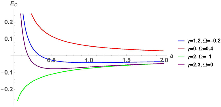
Figure 1. Quantum vacuum energy as a function of the distance a for different values of the δδ′ couplings.

FIGURE 2

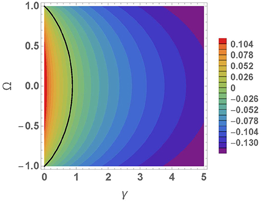
Figure 2. Quantum vacuum energy for a = 0.5 in the coupling space γ-Ω. The black line represents the zero energy curve.

It is interesting to remark that, as it happens for the quantum vacuum interaction energy between two Dirac- δ plates in a 1 + 1 dimensional scalar quantum field theory, the limit

$\begin{array}{ll}{\displaystyle \underset{w_0\to 0}{lim}}{E}_{\delta {\delta }^{\prime }\text{comb}}^{fin}(\Omega =-1,w_0),& (54)\end{array}$

is not analytical in w₀ due to the infrared divergence that appears in the Feymann diagrams (see refs. [22, 23]). This can be seen in (50) if we take into account that the non analyticity is enclosed in the third term of the r.h.s.

6. Conclusions and Further Comments

We calculated the quantum vacuum energy of a comb formed by linear combinations of δ- and δ′-functions given in (1). The method presented in this paper is based on the spectral zeta function. We showed that the δ-δ′ comb with lattice spacing a is equivalent to a single δ-δ′ potential in the interval [−a/2, a/2] at x = 0 together with a 1-parameter family of quasi-periodic boundary conditions at x = ±a/2 given by (22). The band structure (27) arises when one takes into account that the spectrum of the comb is the set obtained by the union of all the discrete spectra of all the selfadjoint extensions obtained from the 1-parameter family of boundary conditions (22). The method can be easily generalized to any comb formed by the repetition of potentials with compact support, as long as the compact support is smaller than the lattice spacing. The ultraviolet divergences of these combs are the same as those of the quantum vacuum energy for one potential with compact support over the real line, which does not have a band structure but a continuum spectrum. Therefore, the ultraviolet divergences for the kind of combs studied in this paper do not depend on the lattice spacing. Subtracting these contributions we get a finite quantum vacuum energy that represents the part of the vacuum expectation value of the Hamiltonian of the quantum field theory, which depends on the lattice spacing. As expected, the generalized vacuum energy vanishes in the limit of infinite lattice spacing. This procedure has already been applied in ref. [24] for two δ-functions. The interpretation of this vacuum energy is a contribution (one-loop quantum correction) to the elastic lattice forces produced by the quantum scalar field of the phonons.

The calculations are to a large extent explicit. The result (51), has a fast converging single integration over k with the integrand (50), given in terms of elementary functions: exponential and hyperbolic functions. This integration is over imaginary frequency after performing a Wick rotation [24]. In addition, the result presented in (51) enables us to infer that when w₁ = 0, i.e., Ω = −1, the function $E_{\delta {\delta }^{\prime }\text{comb}}^{fin}(\Omega =-1,\gamma =w_0)$ is not analytical when w₀ → 0. Moreover, the plot in Figure 3 shows that

$\begin{array}{ll}{E}_{\delta {\delta }^{\prime }\text{comb}}^{fin}(\Omega =-1,w_0\to 0)~w_{0}log{w}_0,& (55)\end{array}$

as known from the vacuum energy of a single delta function (see refs. [22, 23]).

FIGURE 3

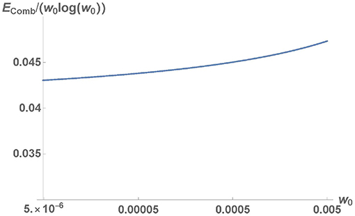
Figure 3. Plot of $E_{\delta {\delta }^{\prime }\text{comb}}^{fin}(\Omega =-1,w_0\to 0)/(w_{0}log{w}_0)$ for a = 1. The w₀ axis is in logarithmic scale.

From this we can conclude that $E_{\delta {\delta }^{\prime }\text{comb}}^{fin}(w_1,w_0)$ does not admit a perturbative expansion in powers of w₀ around w₀ = 0 when w₁ = 0. Hence the result given in formula (51) is non-perturbative in the sense that there is no power series expansion for $E_{\delta {\delta }^{\prime }\text{comb}}^{fin}(\Omega =-1,w_0)$ when w₀ → 0.

With a two-dimensional parameter space (the strength w₀ of the δ-potential and the strength w₁ of the δ′-potential) the quantum vacuum energy can be positive (repulsive force between nodes of the lattice) and negative (attractive force between nodes of the lattice). The interface between the two regimes mentioned is the line of zero quantum vacuum energy in the Ω-γ plane shown in Figure 2.

The techniques developed in this paper have provide a framework to calculate relevant quantities such as the free energy and the entropy at finite temperatures different from zero.

Author Contributions

All authors listed have made a substantial, direct and intellectual contribution to the work, and approved it for publication.

Conflict of Interest Statement

The authors declare that the research was conducted in the absence of any commercial or financial relationships that could be construed as a potential conflict of interest.

Acknowledgments

The authors acknowledge support from the German Research Foundation (DFG) and Universität Leipzig within the program of Open Access Publishing. JMM-C and LS-S are grateful to the Spanish Government-MINECO (MTM2014-57129-C2-1-P) and the Junta de Castilla y León (BU229P18, VA137G18 and VA057U16) for the financial support. JMM-C would like to thank J. Mateos Guilarte, M. Gadella and L. M. Nieto for fruitful discussions. JMM-C dedicates this paper to the memory of professor Jose M. Mu$\tilde{\text{n}}$oz Porras.

Footnotes

1. ^Many of the results of this paper generalize straightforward to any comb built from a superposition of potentials with compact support centered at the lattice points, provided that the compact support of such potentials is smaller than the lattice spacing.

2. ^It is of note that in the interval [−a/2, a/2], the subinterval [−a/2, 0) belongs to one primitive cell, meanwhile the subinterval (0, a/2] belongs to a different primitive cell.

References

1. de L Kronig R, Penney WG. Quantum mechanics of electrons in crystal lattices. Proc R Soc Lond A Math Phys Eng Sci. (1931) 130:499–513.

Google Scholar

2. Gadella M, Negro J, Nieto LM. Bound states and scattering coefficients of the −aδ(x) + bδ′(x) potential. Phys Lett A. (2009) 373:1310–3. doi: 10.1016/j.physleta.2009.02.025

CrossRef Full Text | Google Scholar

3. Muñoz-Castañeda JM, Guilarte JM. δ-δ′ generalized Robin boundary conditions and quantum vacuum fluctuations. Phys Rev. (2015) D91:025028. doi: 10.1103/PhysRevD.91.025028

CrossRef Full Text | Google Scholar

4. Gadella M, Mateos-Guilarte J, Muñoz-Castañeda JM, Nieto LM. Two-point one-dimensional δ-δ′ interactions: non-abelian addition law and decoupling limit. J Phys A Math Theor. (2016) 49:015204. doi: 10.1088/1751-8113/49/1/015204

CrossRef Full Text | Google Scholar

5. Albeverio S, Fassari S, Rinaldi F. A remarkable spectral feature of the Schrödinger Hamiltonian of the harmonic oscillator perturbed by an attractive δ′-interaction centred at the origin: double degeneracy and level crossing. J Phys A Math Theor. (2013) 46:385305. doi: 10.1088/1751-8113/46/38/385305

CrossRef Full Text | Google Scholar

6. Gadella M, Glasser ML, Nieto LM. One dimensional models with a singular potential of the type αδ(x) + βδ′(x). Int J Theor Phys. (2011) 50:2144–52. doi: 10.1007/s10773-010-0641-6

CrossRef Full Text | Google Scholar

7. Gadella M, Glasser ML, Nieto LM. The infinite square well with a singular perturbation. Int J Theor Phys. (2011) 50:2191–200. doi: 10.1007/s10773-011-0690-5

CrossRef Full Text | Google Scholar

8. Nieto LM, Gadella M, Guilarte JM, Muñoz-Castañeda JM, Romaniega C. Towards modelling QFT in real metamaterials: singular potentials and self-adjoint extensions. J Phys Conf Ser. (2017) 839:012007. doi: 10.1088/1742-6596/839/1/012007

CrossRef Full Text | Google Scholar

9. Muñoz-Castañeda JM, Guilarte JM, Mosquera AM. Quantum vacuum energies and Casimir forces between partially transparent δ-function plates. Phys Rev. (2013) D87:105020. doi: 10.1103/PhysRevD.87.105020

CrossRef Full Text | Google Scholar

10. Kirsten K. Spectral Functions in Mathematics and Physics. Boca Raton, FL: Chapman & Hall/CRC (2001).

11. Vassilevich DV. Heat kernel expansion: user's manual. Phys Rep. (2003) 388:279–360. doi: 10.1016/j.physrep.2003.09.002

CrossRef Full Text | Google Scholar

12. Elizalde E. Ten Physical Applications of Spectral Zeta Functions. Lecture Notes in Physics. Berlin; Heidelberg: Springer (2012).

13. Asorey M, Muñoz-Castañeda JM. Attractive and repulsive casimir vacuum energy with general boundary conditions. Nucl Phys. (2013) B874:852–76. doi: 10.1016/j.nuclphysb.2013.06.014

CrossRef Full Text | Google Scholar

14. Muñoz-Castañeda JM, Kirsten K, Bordag M. QFT over the finite line. Heat kernel coefficients, spectral zeta functions and selfadjoint extensions. Lett Math Phys. (2015) 105:523–49. doi: 10.1007/s11005-015-0750-5

CrossRef Full Text | Google Scholar

15. Asorey M, Garcia-Alvarez D, Muñoz-Castañeda JM. Casimir effect and global theory of boundary conditions. J. Phys. A: Math. Gen. (2006) 39:6127–36. doi: 10.1088/0305-4470/39/21/S03

CrossRef Full Text | Google Scholar

16. Ashcroft NW, Mermin ND. Solid State Physics. HRW international ed. Holt; Rinehart and Winston (1976).

17. Asorey M, Muñoz-Castañeda JM. Vacuum boundary effects. Int J Theor Phys. (2011) 50:2211–21. doi: 10.1007/s10773-011-0720-3

CrossRef Full Text | Google Scholar

18. Muñoz-Castañeda JM. Boundary Effects in Quantum Field Theory (in Spanish). Ph.D. Dissertation, Universidad de Zaragoza (2009).

19. Gradshteyn IS, Jeffrey A, Ryzhik IM. Table of Integrals, Series, and Products. Academic Press (1996).

20. Ambjorn J, Wolfram S. Properties of the vacuum. I. Mechanical and thermodynamic. Ann Phys. (1983) 147:1–32.

Google Scholar

21. Elizalde E, Romeo A. Rigorous extension of the proof of zeta-function regularization. Phys Rev D. (1989) 40:436–43.

PubMed Abstract | Google Scholar

22. Toms DJ. Renormalization and vacuum energy for an interacting scalar field in a δ-function potential. J Phys A Math Theor. (2012) 45:374026. doi: 10.1088/1751-8113/45/37/374026

CrossRef Full Text | Google Scholar

23. Milton KA. Casimir energies and pressures for δ-function potentials. J Phys A Math Gen. (2004) 37:6391. doi: 10.1088/0305-4470/37/24/014

CrossRef Full Text | Google Scholar

24. Bordag M, Hennig D, Robaschik D. Vacuum energy in quantum field theory with external potentials concentrated on planes. J Phys A. (1992) A25:4483.

Google Scholar