Numerical Method for Fractional Model of Newell-Whitehead-Segel Equation

The aim of the present work is to devote a friendly approach based on Adomian decomposition method (ADM) to find the numerical solution of the time-fractional Newell-Whitehead-Segel equation. Newell-Whitehead-Segel equation plays an efficient role in non-linear systems which describe the appearance of the stripe patterns in two dimensional systems. The numerical results obtained by proposed method are compared with exact solution for different values of fractional order α. Plotted graph illustrate the efficiency and accuracy of the proposed technique.

AMS Mathematics Subject Classification (2010): 44A99, 35Q99.

Introduction

Fractional calculus is a field of applied mathematics, three centuries old as the conventional calculus. Fractional calculus deals with derivatives and integrals of arbitrary orders. During the last decade, superb improvements have been visualized in the field of fractional calculus, very popular amongst science and engineering community. In recent year, differential equation containing fractional order derivatives has been contributed in various fields of science and engineering [1–4] such as diffusion equation, polarization, electro-magnetic waves, visco elasticity, electrode-electrolyte heat conduction, finance [5], control theory, biomedical engineering, biology [6] etc. In order to achieve the goal of highly accurate solution, many authors illustrate various techniques such as Adomian decomposition method [7], Finite difference method [8], Generalized differential transform method [9], Finite element method [10], Fractional differential transform method [11], Homotopy perturbation method [12, 13], Iterative methods [14], Variational iteration method [15], Homotopy analysis method [16], Differential quadrature method [17], Homotopy perturbation Sumudu transform method [18], Homotopy analysis transform method [19], Local fractional homotopy perturbation Sumudu transform method and Local fractional reduced differential transform method [20], Homotopy analysis Sumudu transform method [21] etc.

Recently various author used a new fractional derivative with Mittag-Leffler type kernel by different numerical method like Laplace decomposition method [22] and iterative method [23] etc.

The Newell-Whitehead-Segel equation model is the interaction of the effect of the diffusion term with the non-linear effect of the reaction term. Fractional Newell-Whitehead-Segel equation is written as

$\begin{array}{ll}{u}_t^{\alpha }=k{u}_{xx}+au-b{u}^q,t>0,0<\alpha \le 1,& (1.1)\end{array}$

where a, b and k > 0 are real numbers and q is a positive integers. First term on the left hand side in Equation (1.1) $u_t^{\alpha }$represent the variation of u(x, t) with time at a fixed location, first term on the right hand side u_xx represent the variation of u(x, t) with spatial variable at a specific time and term au − bu^q takes into account the effect of the source term. The function u(x, t) may be non-linear distribution of temperature in an infinitely thin and long rod or fluid flow as a velocity in an infinitely long pipe with narrow diameter.

Mostly two types of patterns are observed. First is the roll pattern in which cylinders form by fluid stream lines. These cylinders may be bend and form spiral like patterns. Second pattern is the hexagonal in which liquid flow is divided into honey comb cells. The same patterns, stripes and hexagons appear in different physical system. For example, stripes patterns are notice in human fingerprints, on zebra skin and in a visual cortex. Hexagonal patterns are obtained from the propagation of laser beams through a non-linear medium and in systems with chemical reaction and diffusion species [24].

Recently Newell-Whitehead-Segel equations were solved by S. S. Nourazar, M. Soori, and A. Nazari-Golshan by homotopy perturbation method [25], A. Prakash and M. Kumar [26] by He's variational iteration method. Also fractional model of Newell-Whitehead-Segel were solved by Kumar et al. [27] and Prakash et al. [28] by homotopy analysis Sumudu transform method and fractional variational iteration method, respectively. But fractional model of Newell-Whitehead-Segel has not been solved by Adomian decomposition method. Adomian decomposition method is very powerful and efficient numerical method for handling non-linear fractional model. Adomian decomposition method (ADM) demonstrates fast convergence of the solution and therefore provides several significant advantages. This method attacks directly on non-linear term, in a straightforward fashion without using linearization, discretization, perturbation or any other restrictive assumption. Many studies have shown that few terms of decomposition series provide numerical result of high degree of accuracy which makes the method powerful when compared with other existing numerical techniques.

The outline of this paper is as follow. First section is introductory, in the Basic Definition of Fractional Calculus the basic definition of fractional calculus is discussed, in Proposed Adomian Decomposition Method solution process of non-linear Newell-Whitehead-Segel equation by Adomian decomposition method is discussed, in Error Analysis of The Proposed Method error analysis of proposed technique is discussed, in Application of ADM to Fractional Newell-Whitehead-Segel Equation five test examples of fractional Newell-Whitehead-Segel equation are given to elucidate the proposed method ADM and in last Conclusion of the work is drawn.

Basic Definition of Fractional Calculus

In this section, we will introduce the basic definitions and properties of fractional calculus used to describe the proposed schemes.

Definition 2.1. A real function f(t), t > 0, is said to be in the space C_α, ϵ αR, if there exists a real number p, (p > α), such that $f(t)=t^p{f}_1(t),$ where f₁(t) ϵ C[0, ∞) and it is said to be in the space $C_{\alpha }^{m}if{f}^{(m)}ϵC_{\alpha },mϵN\bigcup \left\{0\right\}.$

Definition 2.2. The Riemann-Liouville fractional integral of order α ≥ 0, of a function f(t) ϵ C_β, β ≥ −1 is defined as [29–31]:

$\begin{array}{l}{J}^{\alpha }f(t)=\frac{1}{\Gamma (\alpha )}{\displaystyle {\int }_0^t}\frac{f(\tau )}{{(t-\tau )}^{1-\alpha }}d\tau =\frac{1}{\Gamma (\alpha +1)}{\displaystyle {\int }_0^t}f(\tau ){(d\tau )}^{\alpha },\\ J^{0}f(t)=f(t).\end{array}$

For the Riemann-Liouville fractional integral, we have

$\begin{array}{l}{J}^{\alpha }{t}^{\beta }=\frac{\Gamma (\beta +1)}{\Gamma (\beta +\alpha +1)}{t}^{\alpha +\beta },\end{array}$

where Γ. is the well-known Gamma Function.

Definition 2.3. The Caputo fractional derivative of $f(t),f\in C_{-1}^m,m\in N,m>0,$ is defined as [29–31]:

$\begin{array}{l}{D}^{\alpha }f(t)=I^{m-\alpha }{D}^{m}f(t)=\frac{1}{\Gamma (m-\alpha )}{\displaystyle {\int }_0^t}{(t-x)}^{m-\alpha -1}{f}^m(x)dx,\end{array}$

Where m − 1 < α ≤ m.

Proposed Adomian Decomposition Method

In this section, we illustrate the basic idea of the Adomian Decomposition method (ADM) for the time-fractional Newell-Whitehead-Segel equation.

Consider time-fractional Newell-Whitehead-Segel equation as

$\begin{array}{ll}{u}_t^{\alpha }=k{u}_{xx}+au-b{u}^q,t>0,0<\alpha \le 1,& (3.1)\end{array}$

where a, b and k > 0 are real numbers and q is a positive integers with initial condition

$\begin{array}{l}u(x,0)=f(x,t).\end{array}$

Applying the operator $J_t^{\alpha }$ on both sides of (3.1), we have

$\begin{array}{l}u(x,t)={{\displaystyle \sum }}_{k=0}^{m-1}{(\frac{{\partial }^{k}u}{{\partial t}^k})}_{t=0}\frac{t^k}{\Gamma (k+1)}+J_t^{\alpha }f(x,t)\\ -J_t^{\alpha }(k{u}_{xx}+au-b{u}^q).& (3.2)\end{array}$

Next, we decompose the unknown function u(x, t) into sum of an infinite number of components given by the series

$\begin{array}{ll}u(x,t)={{\displaystyle \sum }}_{n=0}^{\infty }{u}_n(x,t),& (3.3)\end{array}$

and the non-linear term can be decomposed as

$\begin{array}{ll}b{u}^q={{\displaystyle \sum }}_{n=0}^{\infty }{A}_n,& (3.4)\end{array}$

where A_n are Adomian polynomial, given by

$\begin{array}{ll}{A}_n=\frac{1}{\Gamma (n+1)}{\left[\frac{d^n}{d{\lambda }^n}{\left\{b{{\displaystyle \sum }}_{n=0}^{\infty }{\lambda }^i{u}_i(x,t)\right\}}^q\right]}_{\lambda =0},& (3.5)\end{array}$

where n = 0, 1, 2, 3, …….

Components u₀, u₁, u₂, u₃, u₄, …. are determined by substituting (3.3), (3.4), and (3.5) into (3.2) leading to

$\begin{array}{l}{{\displaystyle \sum }}_{n=0}^{\infty }{u}_n(x,t)={{\displaystyle \sum }}_{k=0}^{m-1}{\left(\frac{{\partial }^{k}u}{{\partial t}^k}\right)}_{t=0}\frac{t^k}{\Gamma (k+1)}+J_t^{\alpha }f(x,t)\\ -J_t^{\alpha }\{{k({{\displaystyle \sum }}_{n=0}^{\infty }{u}_n(x,t))}_{xx}+a({{\displaystyle \sum }}_{n=0}^{\infty }{u}_n(x,t))+{{\displaystyle \sum }}_{n=0}^{\infty }{A}_n\}.& (3.6)\end{array}$

This can be written as

$\begin{array}{l}{u}_0+u_1+u_2+\dots ={\displaystyle {\sum }_{k=0}^{m-1}{\left(\frac{{\partial }^{k}u}{\partial t^k}\right)}_{t=0}\frac{t^k}{\Gamma \left(k+1\right)}+}{J}_t^{\alpha }f\left(x,t\right)\\ -J_t^{\alpha }[k\left({(u_0)}_{xx}+{(u_1)}_{xx}+{(u_2)}_{xx}+\dots \right)+a(u_0+u_1+u_2+\dots )\\ +\left(A_0+A_1+A_2+A_3+\dots \right)].\end{array}$

Adomian method uses the formal recursive relations as:

$\begin{array}{l}{u}_0={\displaystyle {\sum }_{k=0}^{m-1}{\left(\frac{{\partial }^{k}u}{\partial t^k}\right)}_{t=0}\frac{t^k}{\Gamma \left(k+1\right)}+}{J}_t^{\alpha }f\left(x,t\right),\\ u_{n+1}=-J_t^{\alpha }\{k{(u_n)}_{xx}+a{u}_n+A_n\},n\ge 0.& (3.7)\end{array}$

Error Analysis of the Proposed Method

Theorem 4.1. If we can find a constant 0 < ε < 1 such that ‖u_m+1(x, t)‖ ≤ ε‖u_m(x, t)‖ for each value of m. Moreover, if the truncated series ${\sum }_{m=0}^r{u}_m(x,t)$ is employed as a numerical solution u(x, t), then the maximum absolute truncated error is determined as

$\begin{array}{l}\Vert u(x,t)-{{\displaystyle \sum }}_{m=0}^r{u}_m(x,t)\Vert \le \frac{{\epsilon }^{r+1}}{(1-\epsilon )}\Vert u_0(x,t)\Vert .\end{array}$

Proof. We have

$\begin{array}{l}\Vert u(x,t)-{{\displaystyle \sum }}_{m=0}^r{u}_m(x,t)\Vert =\Vert {{\displaystyle \sum }}_{m=r+1}^{\infty }{u}_m(x,t)\Vert \\ \le {{\displaystyle \sum }}_{m=r+1}^{\infty }\Vert u_m(x,t)\Vert \\ \le {\sum }_{m=r+1}^{\infty }{\epsilon }^m\Vert u_0(x,t)\Vert \\ \le {(\epsilon )}^{r+1}\left[1+{(\epsilon )}^1+{(\epsilon )}^2+\dots \right]\Vert u_0(x,t)\Vert \\ \le \frac{{\epsilon }^{r+1}}{(1-\epsilon )}\Vert u_0(x,t)\Vert .\end{array}$

Which proves the theorem.

Application of ADM to Fractional Newell-Whitehead-Segel Equation

In this section, five test examples of fractional Newell-Whitehead-Segel equation demonstrate the efficiency of proposed ADM.

Ex. 5.1. We study the linear time-fractional Newell-Whitehead-Segel equation

$\begin{array}{ll}{{\text{u}}_{\text{t}}}^{\alpha }={\text{u}}_{\text{xx}}-2u,\text{ t}>0,0<\alpha \le 1,& (5.1)\end{array}$

with initial condition

$\begin{array}{ll}u(x,0)=e^x.& (5.2)\end{array}$

Applying the operator $J_t^{\alpha }$ on both side of above defined problem, we have

$\begin{array}{l}u(x,t)={{\displaystyle \sum }}_{k=0}^{1-1}{\left(\frac{{\partial }^{k}u}{{\partial t}^k}\right)}_{t=0}\frac{t^k}{\Gamma (k+1)}+J_t^{\alpha }\left\{u_{xx}-2u\right\}.\end{array}$

This gives the following recursive relation:

$\begin{array}{l}{u}_0\left(x,t\right)={\displaystyle {\sum }_{k=0}^{1-1}{\left(\frac{{\partial }^{k}u}{\partial t^k}\right)}_{t=0}\frac{t^k}{\Gamma \left(k+1\right)}},\\ u_{n+1}(x,t)=J_t^{\alpha }\{{(u_n)}_{xx}-2u_n\},n\ge 0.\\ u_0=e^x,\\ u_1=-e^x\frac{t^{\alpha }}{\Gamma (\alpha +1)},\\ u_2=e^x\frac{t^{2\alpha }}{\Gamma (2\alpha +1)},\\ u_3=-e^x\frac{t^{3\alpha }}{\Gamma \left(3\alpha +1\right)},\\ {\displaystyle \sum _{n=0}^{\infty }{u}_n\left(x,t\right)=}{e}^x-e^x\frac{t^{\alpha }}{\Gamma \left(\alpha +1\right)}+e^x\frac{t^{2\alpha }}{\Gamma \left(2\alpha +1\right)}\\ -e^x\frac{t^{3\alpha }}{\Gamma \left(3\alpha +1\right)}+\dots ,\end{array}$

Now, for the standard case when α = 1, we get u(x, t) = e^x−t, which is the exact solution of the classical Newell-Whitehead-Segel equation as obtained by HPM [25] and VIM [26]. Here the numerical results obtained by ADM upto eight terms of approximation and exact solution as shown in Figures 1, 2 are almost identical. It can be observed that as the value of t increases, u decreases, and as x increases, u also increases. Hence, the accuracy of ADM can be enhanced by increasing the number of iterations.

FIGURE 1

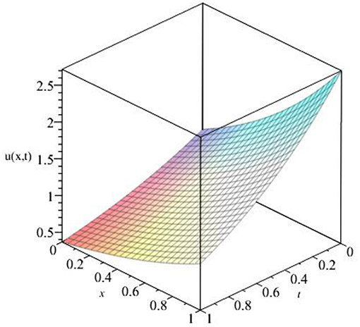
Figure 1. Surface represents eight order approximate solution for α = 1, for Ex. 5.1.

FIGURE 2

Figure 2. Surface represents exact solution for α = 1, for Ex. 5.1.

Ex. 5.2. We study the non-linear time-fractional Newell-Whitehead-Segel equation

$\begin{array}{ll}{u}_t^{\alpha }=u_{xx}+2u-3u^2,t>0,0<\alpha \le 1,& (5.3)\end{array}$

with initial condition

$\begin{array}{ll}u(x,0)=\eta .& (5.4)\end{array}$

Applying the operator $J_t^{\alpha }$ on both side of above defined problem, we have

$\begin{array}{l}u(x,t)={{\displaystyle \sum }}_{k=0}^{1-1}{\left(\frac{{\partial }^{k}u}{{\partial t}^k}\right)}_{t=0}\frac{t^k}{\Gamma (k+1)}+J_t^{\alpha }\left\{u_{xx}+2u+A_n\right\}.\end{array}$

This gives the following recursive relation:

$\begin{array}{l}{u}_0\left(x,t\right)={\displaystyle {\sum }_{k=0}^{1-1}{\left(\frac{{\partial }^{k}u}{\partial t^k}\right)}_{t=0}\frac{t^k}{\Gamma \left(k+1\right)}},\\ u_{n+1}(x,t)=J_t^{\alpha }\{{(u_n)}_{xx}+2u_n+A_n\},n\ge 0.\\ u_0=\eta \\ u_1=\eta (2-3\eta )\frac{t^{\alpha }}{\Gamma (\alpha +1)},\\ u_2=2\eta \left(2-3\eta \right)(1-3\eta )\frac{t^{2\alpha }}{\Gamma (2\alpha +1)},\\ u_3=2\eta \left(2-3\eta \right)(18{\eta }^2-12\eta +2)\frac{t^{3\alpha }}{\Gamma (3\alpha +1)}\\ -3{\eta }^2{\left(2-3\eta \right)}^2\frac{\Gamma \left(2\alpha +1\right)}{\Gamma {\left(\alpha +1\right)}^2}\frac{t^{3\alpha }}{\Gamma \left(3\alpha +1\right)},\\ u_4=-12{\eta }^2\left(2-3\eta \right)\left(18{\eta }^2-12\eta +2\right)\frac{t^{4\alpha }}{\Gamma \left(4\alpha +1\right)}\\ +18{\eta }^3{\left(2-3\eta \right)}^2\frac{\Gamma \left(2\alpha +1\right)}{\Gamma {\left(\alpha +1\right)}^2}\frac{t^{4\alpha }}{\Gamma \left(4\alpha +1\right)}\\ -12{\eta }^2{\left(2-3\eta \right)}^2\left(1-3\eta \right)\frac{\Gamma \left(3\alpha +1\right)}{\Gamma \left(\alpha +1\right)\Gamma \left(2\alpha +1\right)}\frac{t^{4\alpha }}{\Gamma \left(4\alpha +1\right)}\\ +4\eta \left(2-3\eta \right)(18{\eta }^2-12\eta +2)\frac{t^{4\alpha }}{\Gamma (4\alpha +1)}\\ -6{\eta }^2{\left(2-3\eta \right)}^2\frac{\Gamma \left(2\alpha +1\right)}{\Gamma {\left(\alpha +1\right)}^2}\frac{t^{4\alpha }}{\Gamma \left(4\alpha +1\right)}+\dots \\ {\displaystyle \sum _{n=0}^{\infty }{u}_n}\left(x,t\right)=\eta +\eta \left(2-3\eta \right)\frac{t^{\alpha }}{\Gamma \left(\alpha +1\right)}\\ +2\eta \left(2-3\eta \right)\left(1-3\eta \right)\frac{t^{2\alpha }}{\Gamma \left(2\alpha +1\right)}\\ +2\eta \left(2-3\eta \right)\left(18{\eta }^2-12\eta +2\right)\frac{t^{3\alpha }}{\Gamma \left(3\alpha +1\right)}\\ -3{\eta }^2{\left(2-3\eta \right)}^2\frac{\Gamma \left(2\alpha +1\right)}{\Gamma {\left(\alpha +1\right)}^2}\frac{t^{3\alpha }}{\Gamma \left(3\alpha +1\right)}\\ -12{\eta }^2\left(2-3\eta \right)\left(18{\eta }^2-12\eta +2\right)\frac{t^{4\alpha }}{\Gamma \left(4\alpha +1\right)}\\ +18{\eta }^3{\left(2-3\eta \right)}^2\frac{\Gamma \left(2\alpha +1\right)}{\Gamma {\left(\alpha +1\right)}^2}\frac{t^{4\alpha }}{\Gamma \left(4\alpha +1\right)}\\ -12{\eta }^2{\left(2-3\eta \right)}^2\left(1-3\eta \right)\frac{\Gamma \left(3\alpha +1\right)}{\Gamma \left(\alpha +1\right)\Gamma \left(2\alpha +1\right)}\frac{t^{4\alpha }}{\Gamma \left(4\alpha +1\right)}\\ +4\eta \left(2-3\eta \right)(18{\eta }^2-12\eta +2)\frac{t^{4\alpha }}{\Gamma (4\alpha +1)}\\ -6{\eta }^2{\left(2-3\eta \right)}^2\frac{\Gamma \left(2\alpha +1\right)}{\Gamma {\left(\alpha +1\right)}^2}\frac{t^{4\alpha }}{\Gamma \left(4\alpha +1\right)}+\dots \end{array}$

In particular when α = 1, we get the solution in the form

$\begin{array}{l} u(x,t)=\eta +\eta (2-3\eta )t+2\eta (2-3\eta )(1-3\eta )\frac{t^2}{\Gamma (3)}\\ +2\eta (2-3\eta )(27{\eta }^2-18\eta +2)\frac{t^3}{\Gamma (4)}\\ +12\eta (2-3\eta )\left(-54{\eta }^3+54{\eta }^2-14\eta +\frac{2}{3}\right)\frac{t^4}{\Gamma (5)}\dots \dots ,\end{array}$

Which converge to the exact solution of the classical Newell-Whitehead-Segel equation very fastly [25, 26].

$\begin{array}{l}u(x,t)=\frac{\frac{-2}{3}\eta e^{2t}}{-\frac{2}{3}+\eta -\eta e^{2t}}.\end{array}$

Figure 3 shows the comparison of approximate solution for different value of fractional order α = 0.25, 0.50, 0.75, 1 and exact solution at α = 1, when η = 1. It is observed from the Figure 3 that there is a good agreement between exact solution and approximate solution at α = 1. It is also noticed that solution depends on the time-fractional derivative. Accuracy and efficiency can be enhanced by increasing the number of iterations.

FIGURE 3

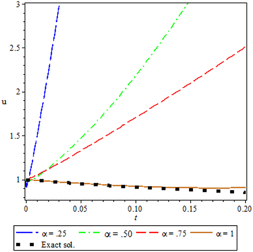
Figure 3. Comparison of approx. sol. for different values of α and exact sol. at α = 1, for Ex. 5.2.

Ex. 5.3. We study the non-linear time-fractional Newell-Whitehead-Segel equation.

$\begin{array}{ll}{u}_t^{\alpha }=u_{xx}+u-u^2=0,t>0,0<\alpha \le 1,& (5.5)\end{array}$

With initial condition,

$\begin{array}{ll}u(x,0)=\frac{1}{{(1+e^{\frac{x}{\sqrt{6}}})}^2}.& (5.6)\end{array}$

Applying the operator $J_t^{\alpha }$ on both side of above equation, we get

$\begin{array}{l}u(x,t)={{\displaystyle \sum }}_{k=0}^{1-1}{\left(\frac{{\partial }^{k}u}{{\partial t}^k}\right)}_{t=0}\frac{t^k}{\Gamma (k+1)}+J_t^{\alpha }\left\{u_{xx}+u+A_n\right\}.\end{array}$

This gives the following recursive relation:

$\begin{array}{l}{u}_0\left(x,t\right)={\displaystyle {\sum }_{k=0}^{1-1}{\left(\frac{{\partial }^{k}u}{\partial t^k}\right)}_{t=0}\frac{t^k}{\Gamma \left(k+1\right)}},\\ u_{n+1}(x,t)=J_t^{\alpha }\{{(u_n)}_{xx}+2u_n+A_n\},n\ge 0.\\ u_0=\frac{1}{{(1+e^{\frac{x}{\sqrt{6}}})}^2},\\ u_1=\frac{5}{3}\frac{e^{\frac{x}{\sqrt{6}}}}{{(1+e^{\frac{x}{\sqrt{6}}})}^3}\frac{t^{\alpha }}{\Gamma (\alpha +1)},\\ u_2=\frac{25}{18}(\frac{e^{\frac{x}{\sqrt{6}}}\left(-1+2e^{\frac{x}{\sqrt{6}}}\right)}{{\left(1+e^{\frac{x}{\sqrt{6}}}\right)}^4})\frac{t^{2\alpha }}{\Gamma (2\alpha +1)},\\ u_3=\{\frac{25}{18}\frac{1}{{\left(1+e^{\frac{x}{\sqrt{6}}}\right)}^5}[\frac{8}{6}{(e^{\frac{x}{\sqrt{6}}})}^2-4{(e^{\frac{x}{\sqrt{6}}})}^3\\ +\left(\frac{8}{6}{(e^{\frac{x}{\sqrt{6}}})}^2-\frac{(e^{\frac{x}{\sqrt{6}}})}{6}\right)\left(1+e^{\frac{x}{\sqrt{6}}}\right)\\ +\frac{4}{6}{(e^{\frac{x}{\sqrt{6}}})}^2-\frac{16}{6}{(e^{\frac{x}{\sqrt{6}}})}^3+\left(2{(e^{\frac{x}{\sqrt{6}}})}^2-e^{\frac{x}{\sqrt{6}}}\right)\left(1+e^{\frac{x}{\sqrt{6}}}\right)\\ +\frac{\frac{-20}{6}{(e^{\frac{x}{\sqrt{6}}})}^3+\frac{40}{6}{(e^{\frac{x}{\sqrt{6}}})}^4}{\left(1+e^{\frac{x}{\sqrt{6}}}\right)}\\ -2(\frac{{(-e^{\frac{x}{\sqrt{6}}})}^1+2{(e^{\frac{x}{\sqrt{6}}})}^2}{\left(1+e^{\frac{x}{\sqrt{6}}}\right)})]\}\frac{t^{3\alpha }}{\Gamma \left(3\alpha +1\right)}-\frac{25}{9}\frac{{(e^{\frac{x}{\sqrt{6}}})}^2}{{\left(1+e^{\frac{x}{\sqrt{6}}}\right)}^6}\\ \frac{\Gamma \left(2\alpha +1\right)t^{3\alpha }}{\Gamma \left(3\alpha +1\right)\Gamma {\left(\alpha +1\right)}^2}.\\ {\displaystyle \sum _{n=0}^{\infty }{u}_n}\left(x,t\right)=\frac{1}{{\left(1+e^{\frac{x}{\sqrt{6}}}\right)}^2}+\frac{5}{3}\frac{e^{\frac{x}{\sqrt{6}}}}{{\left(1+e^{\frac{x}{\sqrt{6}}}\right)}^3}\frac{t^{\alpha }}{\Gamma \left(\alpha +1\right)}\\ +\frac{25}{18}\left(\frac{e^{\frac{x}{\sqrt{6}}}\left(-1+2e^{\frac{x}{\sqrt{6}}}\right)}{{\left(1+e^{\frac{x}{\sqrt{6}}}\right)}^4}\right)\frac{t^{2\alpha }}{\Gamma \left(2\alpha +1\right)}\\ +\{\frac{25}{18}\frac{1}{{\left(1+e^{\frac{x}{\sqrt{6}}}\right)}^5}[\frac{8}{6}{(e^{\frac{x}{\sqrt{6}}})}^2-4{(e^{\frac{x}{\sqrt{6}}})}^3\\ +\left(\frac{8}{6}{(e^{\frac{x}{\sqrt{6}}})}^2-\frac{(e^{\frac{x}{\sqrt{6}}})}{6}\right)\left(1+e^{\frac{x}{\sqrt{6}}}\right)\\ +\frac{4}{6}{(e^{\frac{x}{\sqrt{6}}})}^2-\frac{16}{6}{(e^{\frac{x}{\sqrt{6}}})}^3+\left(2{(e^{\frac{x}{\sqrt{6}}})}^2-e^{\frac{x}{\sqrt{6}}}\right)\left(1+e^{\frac{x}{\sqrt{6}}}\right)\\ +\frac{\frac{-20}{6}{(e^{\frac{x}{\sqrt{6}}})}^3+\frac{40}{6}{(e^{\frac{x}{\sqrt{6}}})}^4}{\left(1+e^{\frac{x}{\sqrt{6}}}\right)}\end{array}$

$\begin{array}{l}-2(\frac{{(-e^{\frac{x}{\sqrt{6}}})}^1+2{(e^{\frac{x}{\sqrt{6}}})}^2}{\left(1+e^{\frac{x}{\sqrt{6}}}\right)})]\}\frac{t^{3\alpha }}{\Gamma \left(3\alpha +1\right)}-\frac{25}{9}\frac{{(e^{\frac{x}{\sqrt{6}}})}^2}{{\left(1+e^{\frac{x}{\sqrt{6}}}\right)}^6}\\ \frac{\Gamma \left(2\alpha +1\right)t^{3\alpha }}{\Gamma \left(3\alpha +1\right)\Gamma {\left(\alpha +1\right)}^2}+\dots \end{array}$

In particular when α = 1, we get the solution in the form

$\begin{array}{l}u\left(x,t\right)=\frac{1}{{\left(1+e^{\frac{x}{\sqrt{6}}}\right)}^2}+\frac{5}{3}\frac{e^{\frac{x}{\sqrt{6}}}}{{\left(1+e^{\frac{x}{\sqrt{6}}}\right)}^3}\frac{t}{1}\\ +\frac{25}{18}\left(\frac{e^{\frac{x}{\sqrt{6}}}\left(-1+2e^{\frac{x}{\sqrt{6}}}\right)}{{\left(1+e^{\frac{x}{\sqrt{6}}}\right)}^4}\right)\frac{t^2}{2}\\ +\left(\frac{125}{216}\frac{(e^{\frac{x}{\sqrt{6}}}(4{\left(e^{\frac{x}{\sqrt{6}}}\right)}^2-7e^{\frac{x}{\sqrt{6}}}+1)}{{\left(1+e^{\frac{x}{\sqrt{6}}}\right)}^5}\right)\frac{t^3}{3}+\dots .\end{array}$

Which converge to the exact solution of the classical Newell-Whitehead-Segel equation very fastly [25].

$\begin{array}{l}u(x,t)=\frac{1}{{\left(1+e^{\frac{x}{\sqrt{6}}-\frac{5}{6}t}\right)}^2}.\end{array}$

Figure 4 shows the comparison of third order approximate solution for different value of fractional order α = 0.25, 0.50, 0.75, 1 and exact solution at α = 1, for x = 1. It is observed from the Figure 4 that there is a good agreement between exact solution and approximate solution at α = 1. It is also noticed that solution depends on the time-fractional derivative. Accuracy and efficiency can be enhanced by increasing the number of iterations.

FIGURE 4

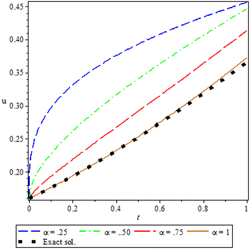
Figure 4. Comparison of approx. sol. for different values of fractional order α and exact sol. at α = 1, for Ex. 5.3.

Ex. 5.4. We study the non-linear time-fractional Newell-Whitehead-Segel equation

$\begin{array}{ll}{u}_t^{\alpha }=u_{xx}+u-u^4=0,t>0,0<\alpha \le 1,& (5.7)\end{array}$

with initial condition

$\begin{array}{ll}u(x,0)={(\frac{1}{1+e^{\frac{3x}{\sqrt{10}}}})}^{\frac{2}{3}}.& (5.8)\end{array}$

Applying the operator $J_t^{\alpha }$ on both side of above equation, we have

$\begin{array}{l}u(x,t)={{\displaystyle \sum }}_{k=0}^{1-1}{\left(\frac{{\partial }^{k}u}{{\partial t}^k}\right)}_{t=0}\frac{t^k}{\Gamma (k+1)}+J_t^{\alpha }\left\{u_{xx}+u+A_n\right\}.\end{array}$

This gives the following recursive relation:

$\begin{array}{l}{u}_0\left(x,t\right)={\displaystyle {\sum }_{k=0}^{1-1}{\left(\frac{{\partial }^{k}u}{\partial t^k}\right)}_{t=0}\frac{t^k}{\Gamma \left(k+1\right)}},\\ u_{n+1}(x,t)=J_t^{\alpha }\{{(u_n)}_{xx}+u_n+A_n\},n\ge 0.\\ u_0={(\frac{1}{1+e^{\frac{3x}{\sqrt{10}}}})}^{\frac{2}{3}},\\ u_1=\frac{7}{5}(\frac{e^{\frac{3x}{\sqrt{10}}}}{{(1+e^{\frac{3x}{\sqrt{10}}})}^{\frac{5}{3}}})\frac{t^{\alpha }}{\Gamma (\alpha +1)},\\ u_2=\frac{49}{50}\{\frac{e^{\frac{3x}{\sqrt{10}}}\left(2e^{\frac{3x}{\sqrt{10}}}-3\right)}{{\left(1+e^{\frac{3x}{\sqrt{10}}}\right)}^{\frac{8}{3}}}\}\frac{t^{2\alpha }}{\Gamma (2\alpha +1)},\\ u_3=\frac{1}{{\left(1+e^{\frac{3x}{\sqrt{10}}}\right)}^{\frac{11}{3}}}\{\frac{3528}{500}{\left(e^{\frac{3x}{\sqrt{10}}}\right)}^2\left(1+e^{\frac{3x}{\sqrt{10}}}\right)\\ -\frac{4704}{500}{(e^{\frac{3x}{\sqrt{10}}})}^3\\ -\frac{1323}{500}(e^{\frac{3x}{\sqrt{10}}})\left(1+e^{\frac{3x}{\sqrt{10}}}\right)\text{}+\text{}\frac{3528}{500}{\left(e^{\frac{3x}{\sqrt{10}}}\right)}^2\text{}-\text{}\frac{7056}{500}{(e^{\frac{3x}{\sqrt{10}}})}^3\end{array}$

$\begin{array}{l}+\frac{7056}{500}{\left(e^{\frac{3x}{\sqrt{10}}}\right)}^2+\frac{8624}{500}\frac{{\left(e^{\frac{3x}{\sqrt{10}}}\right)}^4}{\left(1+e^{\frac{3x}{\sqrt{10}}}\right)}\\ -\frac{12936}{500}\frac{{(e^{\frac{3x}{\sqrt{10}}})}^3}{\left(1+e^{\frac{3x}{\sqrt{10}}}\right)}\\ +\frac{49}{50}\left(2{\left(e^{\frac{3x}{\sqrt{10}}}\right)}^2-3e^{\frac{3x}{\sqrt{10}}}\right)\left(1+e^{\frac{3x}{\sqrt{10}}}\right)\\ -\frac{\frac{196}{50}\left(2{\left(e^{\frac{3x}{\sqrt{10}}}\right)}^2-3e^{\frac{3x}{\sqrt{10}}}\right)}{\left(1+e^{\frac{3x}{\sqrt{10}}}\right)}\}\frac{t^{3\alpha }}{\Gamma \left(3\alpha +1\right)}\\ -\frac{294}{25}\frac{{(e^{\frac{3x}{\sqrt{10}}})}^2}{{(1+e^{\frac{3x}{\sqrt{10}}})}^{\frac{14}{3}}}\frac{\Gamma \left(2\alpha +1\right)t^{3\alpha }}{\Gamma \left(3\alpha +1\right)\Gamma {\left(\alpha +1\right)}^2},\\ {\displaystyle \sum _{n=0}^{\infty }{u}_n}\left(x,t\right)={\left(\frac{1}{1+e^{\frac{3x}{\sqrt{10}}}}\right)}^{\frac{2}{3}}+\frac{7}{5}(\frac{e^{\frac{3x}{\sqrt{10}}}}{{\left(1+e^{\frac{3x}{\sqrt{10}}}\right)}^{\frac{5}{3}}})\\ \frac{t^{\alpha }}{\Gamma \left(\alpha +1\right)}\\ +\frac{49}{50}\left(\frac{e^{\frac{3x}{\sqrt{10}}}\left(2e^{\frac{3x}{\sqrt{10}}}-3\right)}{{\left(1+e^{\frac{3x}{\sqrt{10}}}\right)}^{\frac{8}{3}}}\right)\frac{t^{2\alpha }}{\Gamma \left(2\alpha +1\right)}\\ +\frac{1}{{\left(1+e^{\frac{3x}{\sqrt{10}}}\right)}^{\frac{11}{3}}}\{\frac{3528}{500}{\left(e^{\frac{3x}{\sqrt{10}}}\right)}^2\left(1+e^{\frac{3x}{\sqrt{10}}}\right)\\ -\frac{4704}{500}{(e^{\frac{3x}{\sqrt{10}}})}^3-\frac{1323}{500}(e^{\frac{3x}{\sqrt{10}}})\left(1+e^{\frac{3x}{\sqrt{10}}}\right)\\ +\frac{3528}{500}{\left(e^{\frac{3x}{\sqrt{10}}}\right)}^2\\ -\frac{7056}{500}{(e^{\frac{3x}{\sqrt{10}}})}^3+\frac{7056}{500}{\left(e^{\frac{3x}{\sqrt{10}}}\right)}^2+\frac{8624}{500}\frac{{\left(e^{\frac{3x}{\sqrt{10}}}\right)}^4}{\left(1+e^{\frac{3x}{\sqrt{10}}}\right)}\end{array}$

$-\frac{12936}{500}\frac{{(e^{\frac{3x}{\sqrt{10}}})}^3}{\left(1+e^{\frac{3x}{\sqrt{10}}}\right)}+\frac{49}{50}\left(2{\left(e^{\frac{3x}{\sqrt{10}}}\right)}^2-3e^{\frac{3x}{\sqrt{10}}}\right)\left(1+e^{\frac{3x}{\sqrt{10}}}\right)$

$\begin{array}{l}-\frac{196}{50}\frac{\left(2{\left(e^{\frac{3x}{\sqrt{10}}}\right)}^2-3e^{\frac{3x}{\sqrt{10}}}\right)}{\left(1+e^{\frac{3x}{\sqrt{10}}}\right)}\frac{t^{3\alpha }}{\Gamma \left(3\alpha +1\right)}\}\\ -\frac{294}{25}\frac{{\left(e^{\frac{3x}{\sqrt{10}}}\right)}^2}{{\left(1+e^{\frac{3x}{\sqrt{10}}}\right)}^{\frac{14}{3}}}\frac{\Gamma \left(2\alpha +1\right)t^{3\alpha }}{\Gamma \left(3\alpha +1\right)\Gamma {\left(\alpha +1\right)}^2}\\ +{\dots }_{.}\end{array}$

Taking α = 1, we get the solution in the form

$\begin{array}{l}u(x,t)={\left(\frac{1}{1+e^{\frac{3x}{\sqrt{10}}}}\right)}^{\frac{2}{3}}+\frac{7}{5}(\frac{e^{\frac{3x}{\sqrt{10}}}}{{\left(1+e^{\frac{3x}{\sqrt{10}}}\right)}^{\frac{5}{3}}})\frac{t}{1}\\ +\frac{49}{50}\left(\frac{e^{\frac{3x}{\sqrt{10}}}\left(2e^{\frac{3x}{\sqrt{10}}}-3\right)}{{\left(1+e^{\frac{3x}{\sqrt{10}}}\right)}^{\frac{8}{3}}}\right)\frac{t^2}{2}\\ +\frac{343}{1000}\left(\frac{\left(4{\left(e^{\frac{3x}{\sqrt{10}}}\right)}^2-27e^{\frac{3x}{\sqrt{10}}}+9\right)e^{\frac{3x}{\sqrt{10}}}}{{\left(1+e^{\frac{3x}{\sqrt{10}}}\right)}^{\frac{11}{3}}}\right)\frac{t^3}{3}+\dots .,\end{array}$

Which converge to the exact solution of the classical Newell-Whitehead-Segel equation very fastly [25, 26].

$\begin{array}{l}u(x,t)={[\frac{1}{2}tanh\left(-\frac{3}{2\sqrt{10}}\left(x-\frac{7}{\sqrt{10}}t\right)\right)+\frac{1}{2}]}^{\frac{2}{3}}.\end{array}$

Figure 5 shows the comparison of third order approximate solution for different value of fractional order α = 0.25, 0.50, 0.75, 1 and exact solution at α = 1 for x = 1. It is observed from the Figure 5 that there is a good agreement between exact solution and approximate solution at α = 1. It is also noticed that solution depends on the time-fractional derivative. Accuracy and efficiency can be enhanced by increasing the number of iterations.

FIGURE 5

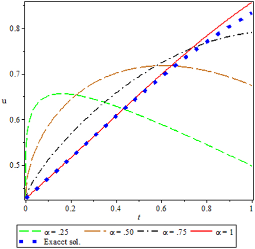
Figure 5. Comparison of approx. sol. for different values of α and exact sol. at α = 1, for Ex. 5.4.

Ex. 5.5. We study the nonlinear time-fractional Newell-Whitehead-Segel equation of the form

$\begin{array}{ll}{u}_t^{\alpha }=u_{xx}+3u-{4u}^4=0,t>0,0<\alpha \le 1,& (5.9)\end{array}$

with initial condition

$\begin{array}{ll}u(x,0)=\sqrt{\frac{3}{4}}\frac{e^{\sqrt{6}x}}{e^{\sqrt{6}x}+e^{\frac{\sqrt{6}}{2}x}}.& (5.10)\end{array}$

Applying the operator $J_t^{\alpha }$ on both side of above defined problem, we have

$\begin{array}{l}u(x,t)={{\displaystyle \sum }}_{k=0}^{1-1}{\left(\frac{{\partial }^{k}u}{{\partial t}^k}\right)}_{t=0}\frac{t^k}{\Gamma (k+1)}+J_t^{\alpha }\left\{u_{xx}+2u+A_n\right\}.\end{array}$

This gives the following recursive relation:

$\begin{array}{l}{u}_0\left(x,t\right)={\displaystyle {\sum }_{k=0}^{1-1}{\left(\frac{{\partial }^{k}u}{\partial t^k}\right)}_{t=0}\frac{t^k}{\Gamma \left(k+1\right)}},\\ u_{n+1}(x,t)=J_t^{\alpha }\{{(u_n)}_{xx}+3u_n+A_n\},n\ge 0.\\ u_0=\sqrt{\frac{3}{4}}\frac{e^{\sqrt{6}x}}{e^{\sqrt{6}x}+e^{\frac{\sqrt{6}}{2}x}},\\ u_1=\frac{9}{2}\sqrt{\frac{3}{4}}\frac{e^{\sqrt{6}x}{e}^{\frac{\sqrt{6}}{2}x}}{{(e^{\sqrt{6}x}+e^{\frac{\sqrt{6}}{2}x})}^2}\frac{t^{\alpha }}{\Gamma (\alpha +1)},\\ u_2=\frac{81}{4}\sqrt{\frac{3}{4}(}\frac{e^{\sqrt{6}x}{e}^{\frac{\sqrt{6}}{2}x}\left(-e^{\sqrt{6}x}+e^{\frac{\sqrt{6}}{2}x}\right)}{{(e^{\sqrt{6}x}+e^{\frac{\sqrt{6}}{2}x})}^3})\frac{t^{2\alpha }}{\Gamma (2\alpha +1)},\\ u_3=\frac{81}{4}\sqrt{\frac{3}{4}}\frac{1}{{\left(1+e^{-\frac{\sqrt{6}}{2}x}\right)}^4}\{-\frac{3}{2}\left(e^{-\frac{\sqrt{6}}{2}x}\right)\left(1+e^{-\frac{\sqrt{6}}{2}x}\right)\\ +\frac{9}{2}{\left(e^{-\frac{\sqrt{6}}{2}x}\right)}^2\\ +6{\left(e^{-\frac{\sqrt{6}}{2}x}\right)}^2\left(1+e^{-\frac{\sqrt{6}}{2}x}\right)-9{\left(e^{-\frac{\sqrt{6}}{2}x}\right)}^3+9{\left(e^{-\frac{\sqrt{6}}{2}x}\right)}^2\\ -18\frac{{\left(e^{-\frac{\sqrt{6}}{2}x}\right)}^3}{\left(1+e^{-\frac{\sqrt{6}}{2}x}\right)}\\ -\frac{27}{2}{\left(e^{-\frac{\sqrt{6}}{2}x}\right)}^3+18\frac{{\left(e^{-\frac{\sqrt{6}}{2}x}\right)}^4}{\left(1+e^{-\frac{\sqrt{6}}{2}x}\right)}+3(-e^{-\frac{\sqrt{6}}{2}x}\\ +{\left(e^{-\frac{\sqrt{6}}{2}x}\right)}^2)\left(1+e^{-\frac{\sqrt{6}}{2}x}\right)\\ -9\frac{e^{-\frac{\sqrt{6}}{2}x}(-1+e^{-\frac{\sqrt{6}}{2}x})}{(1+e^{-\frac{\sqrt{6}}{2}x})}\}\frac{t^{3\alpha }}{\Gamma (3\alpha +1)}-\frac{729}{4}\\ \sqrt{\frac{3}{4}}\frac{{(-e^{-\frac{\sqrt{6}}{2}x})}^2}{{(1+e^{-\frac{\sqrt{6}}{2}x})}^5}\frac{\Gamma \left(2\alpha +1\right)t^{3\alpha }}{\Gamma \left(3\alpha +1\right)\Gamma {\left(\alpha +1\right)}^2},\\ {\displaystyle \sum _{n=0}^{\infty }{u}_n}\left(x,t\right)=\sqrt{\frac{3}{4}}\frac{e^{\sqrt{6}x}}{e^{\sqrt{6}x}+e^{\frac{\sqrt{6}}{2}x}}\\ +\frac{9}{2}\sqrt{\frac{3}{4}}\frac{e^{\sqrt{6}x}{e}^{\frac{\sqrt{6}}{2}x}}{{(e^{\sqrt{6}x}+e^{\frac{\sqrt{6}}{2}x})}^2}\frac{t^{\alpha }}{\Gamma \left(\alpha +1\right)}\\ +\frac{81}{4}\sqrt{\frac{3}{4}}\frac{e^{\sqrt{6}x}{e}^{\frac{\sqrt{6}}{2}x}\left(-e^{\sqrt{6}x}+e^{\frac{\sqrt{6}}{2}x}\right)}{{(e^{\sqrt{6}x}+e^{\frac{\sqrt{6}}{2}x})}^3}\frac{t^{2\alpha }}{\Gamma \left(2\alpha +1\right)}\\ +\frac{81}{4}\sqrt{\frac{3}{4}}\frac{1}{{\left(1+e^{-\frac{\sqrt{6}}{2}x}\right)}^4}\{-\frac{3}{2}\left(e^{-\frac{\sqrt{6}}{2}x}\right)\\ {}^{\ast }\left(1+e^{-\frac{\sqrt{6}}{2}x}\right)+\frac{9}{2}{\left(e^{-\frac{\sqrt{6}}{2}x}\right)}^2++6{\left(e^{-\frac{\sqrt{6}}{2}x}\right)}^2\left(1+e^{-\frac{\sqrt{6}}{2}x}\right)\\ -9{\left(e^{-\frac{\sqrt{6}}{2}x}\right)}^3+9{\left(e^{-\frac{\sqrt{6}}{2}x}\right)}^2\\ -18\frac{{\left(e^{-\frac{\sqrt{6}}{2}x}\right)}^3}{\left(1+e^{-\frac{\sqrt{6}}{2}x}\right)}-\frac{27}{2}{\left(e^{-\frac{\sqrt{6}}{2}x}\right)}^3+18\frac{{\left(e^{-\frac{\sqrt{6}}{2}x}\right)}^4}{\left(1+e^{-\frac{\sqrt{6}}{2}x}\right)}\\ +3\left(-e^{-\frac{\sqrt{6}}{2}x}+{\left(e^{-\frac{\sqrt{6}}{2}x}\right)}^2\right)\\ {}^{\ast }\left(1+e^{-\frac{\sqrt{6}}{2}x}\right)-9\frac{e^{-\frac{\sqrt{6}}{2}x}\left(-1+e^{-\frac{\sqrt{6}}{2}x}\right)}{\left(1+e^{-\frac{\sqrt{6}}{2}x}\right)}\}\frac{t^{3\alpha }}{\Gamma \left(3\alpha +1\right)}\\ -\frac{729}{4}\sqrt{\frac{3}{4}}\frac{{\left(-e^{-\frac{\sqrt{6}}{2}x}\right)}^2}{{\left(1+e^{-\frac{\sqrt{6}}{2}x}\right)}^5}\frac{\Gamma \left(2\alpha +1\right)t^{3\alpha }}{\Gamma \left(3\alpha +1\right)\Gamma {\left(\alpha +1\right)}^2}+\dots \end{array}$

Taking α = 1, we get the solution in the form

$\begin{array}{l}u(x,t)=\sqrt{\frac{3}{4}}\frac{e^{\sqrt{6}x}}{e^{\sqrt{6}x}+e^{\frac{\sqrt{6}}{2}x}}+\frac{9}{2}\sqrt{\frac{3}{4}}\frac{e^{\sqrt{6}x}{e}^{\frac{\sqrt{6}}{2}x}}{{(e^{\sqrt{6}x}+e^{\frac{\sqrt{6}}{2}x})}^2}\frac{t}{1}\hfill \\ +\frac{81}{4}\sqrt{\frac{3}{4}}\frac{e^{\sqrt{6}x}{e}^{\frac{\sqrt{6}}{2}x}(-e^{\sqrt{6}x}+e^{\frac{\sqrt{6}}{2}x})}{{(e^{\sqrt{6x}}+e^{\frac{\sqrt{6}}{2}x})}^3}\frac{t^2}{2}\hfill \\ +\frac{243}{16}\sqrt{\frac{3}{4}}\frac{e^{\sqrt{6}x}{e}^{\frac{\sqrt{6}}{2}x}\left(-4e^{\sqrt{6}x}{e}^{\frac{\sqrt{6}}{2}x}+{(e^{\sqrt{6}x})}^2+{(e^{\frac{\sqrt{6}}{2}x})}^2\right)}{{(e^{\sqrt{6}x}+e^{\frac{\sqrt{6}}{2}{x}^4})}^4}\frac{t^3}{3}\hfill \\ +\dots \hfill \end{array}$

which converge to the exact solution of the classical Newell-Whitehead-Segel equation very fastly [25, 26].

$\begin{array}{l}u(x,t)=\sqrt{\frac{3}{4}}\frac{e^{\sqrt{6}x}}{e^{\sqrt{6}x}+e^{(\frac{\sqrt{6}}{2}x-\frac{9}{2}t)}}.\end{array}$

Figure 6 shows the comparison of third order approximate solution for different value of fractional order α = 0.25, 0.50, 0.75, 1 and exact solution at α = 1, for x = 1. It is observed from the Figure 6 that there is a good agreement between exact solution and approximate solution at α = 1. It is also noticed that solution depends on the time-fractional derivative. Accuracy and efficiency can be enhanced by increasing the number of iterations.

FIGURE 6

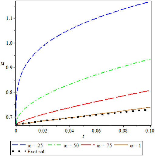
Figure 6. Comparison of approx. sol. for different values of fractional order α and exact sol. at α = 1, for Ex. 5.5.

Conclusion

In this article, we have successfully applied the ADM to obtain the approximate analytic solutions of fractional model of Newell-Whitehead-Segel equation. The plotted graph and numerical result shows the accuracy of proposed method. We observed an excellent agreement between ADM and the exact solution. The results reveal that ADM is an efficient and computationally very attractive approach to investigate non-linear fractional model. Therefore, ADM can be further applied to solve various types of linear and non-linear fractional model arising in the field of science and engineering.

Author Contributions

AP and VV designed the study, collected the data, performed the analysis, and wrote the manuscript.

Conflict of Interest Statement

The authors declare that the research was conducted in the absence of any commercial or financial relationships that could be construed as a potential conflict of interest.

References

1. Oldham KB, Spanier J. The Fractional Calculus: Theory and applications of Differentiation and Integration of Arbitrary Order. New York, NY: Academic Press (1974).

Google Scholar

2. Podlubny I. Fractional Differential Equation. New York, NY: Academic Press (1999).

3. Jain S. Numerical analysis for the fractional diffusion and fractional Buckmaster's equation by two step Adam-Bashforth method. Eur Phy J Plus (2018) 133:19. doi: 10.1140/epjp/i2018-11854-x

CrossRef Full Text | Google Scholar

4. Magin RL. Fractional Calculus in Bioengineering. New York, NY: Begell House Publishers (2006).

Google Scholar

5. Raberto M, Scalas M, Mainardi F. Waiting times and returns in high frequency financial data. An empirical study. Phys A (2002) 314:749–55. doi: 10.1016/S0378-4371(02)01048-8

CrossRef Full Text | Google Scholar

6. Momani S, Odibat Z. Numerical approach to differential equations of fractional orders. J Comput Appl Math. (2007) 207:96–110. doi: 10.1016/j.cam.2006.07.015

CrossRef Full Text | Google Scholar

7. Ray SS, Bera RK. Analytical solution of Bagley–Torvik equation by Adomian decomposition method. Appl Math Comput. (2005) 168:398–410. doi: 10.1016/j.amc.2004.09.006

CrossRef Full Text | Google Scholar

8. Meerschaert M, Tadjeran C. Finite difference approximations for two sided space fractional partial differential equations. Appl Numer Math. (2006) 56:80–90. doi: 10.1016/j.apnum.2005.02.008

CrossRef Full Text | Google Scholar

9. Odibat Z, Momani S, Erturk VS. Generalized differential transform method: application to differential equations of fractional order. Appl Math Comput. (2008) 197:467–77. doi: 10.1016/j.amc.2007.07.068

CrossRef Full Text | Google Scholar

10. Jiang Y, Ma J. Higher order finite element methods for time-fractional partial differential equations. J Comput Appl Math. (2011) 235:3285–90. doi: 10.1016/j.cam.2011.01.011

CrossRef Full Text | Google Scholar

11. Arikoglu A, Ozkol I. Solution of a fractional differential equations by using differential transform method. Chaos Solitons Fract. (2007) 34:1473–81. doi: 10.1016/j.chaos.2006.09.004

CrossRef Full Text | Google Scholar

12. Zhang X. Homotopy perturbation method for two dimensional time-fractional wave equation. Appl Math Model. (2014) 38:5545–52. doi: 10.1016/j.apm.2014.04.018

CrossRef Full Text | Google Scholar

13. Prakash A. Analytical method for space-fractional telegraph equation by homotopy perturbation transform method. Nonlin Eng. (2016) 5:123–8. doi: 10.1515/nleng-2016-0008

CrossRef Full Text | Google Scholar

14. Dhaigude CD, Nikam VR. Solution of fractional partial differential equations using iterative method. Fract Calc Appl Anal. (2012) 15:684–99. doi: 10.2478/S13540-012-0046-8

CrossRef Full Text | Google Scholar

15. Safari M, Ganji DD, Moslemi M. Application of He's Variational iteration method and Adomain decomposition method to the fractional KdV-Burger-Kuramoto equation. Comput Appl. (2009) 58:2091–97. doi: 10.1016/j.camwa.2009.03.043

CrossRef Full Text | Google Scholar

16. Liao S. On the homotopy analysis method for nonlinear problem. Appl Math Comput. (2004) 147:499–513. doi: 10.1016/S0096-3003(02)00790-7

CrossRef Full Text | Google Scholar

17. Jiwari R, Pandit S, Mittal RC. Numerical solution of two dimensional Sine-Gordon Solitons by Differential Quadrature method. Comput Phys Commun. (2012) 183:600–16. doi: 10.1016/j.cpc.2011.12.004

CrossRef Full Text | Google Scholar

18. Singh J, Kumar D. Homotopy perturbation Sumudu transform method for nonlinear equation. Adv Appl Mech. (2011) 14:165–75.

Google Scholar

19. Kumar D, Singh J, Baleanu D, Rathore S. Analysis of fractional model of Ambartsumian equation. Eur Phy J Plus (2018) 133:259. doi: 10.1140/epjp/i2018-12081-3

CrossRef Full Text | Google Scholar

20. Kumar D, Tichier F, Singh J, Baleanu D. An efficient computational technique for fractal vehicular traffic flow. Entropy (2018) 20:259. doi: 10.3390/e20040259

CrossRef Full Text | Google Scholar

21. Singh J, Kumar D, Baleanu D, Rathore S. An efficient numerical algorithm for the fractional Drinfeld-Sokolov-Wilson equation. Appl Math Comput. (2019) 335:12–24. doi: 10.1016/j.amc.2018.04.025

CrossRef Full Text | Google Scholar

22. Kumar D, Singh J, Baleanu D. A new analysis of Fornberg-Whitham equation pertaining to a fractional derivative with Mittag-Leffler type kernel. Eur Phy J Plus (2018) 133:70. doi: 10.1140/epjp/i2018-11934-y

CrossRef Full Text | Google Scholar

23. Kumar D, Singh J, Baleanu D. The analysis of chemical kinetics system pertaining to a fractional derivative with Mittag-Leffler type kernel. Chaos (2017) 27:103113. doi: 10.1063/1.4995032

PubMed Abstract | CrossRef Full Text | Google Scholar

24. Golovinb NA. General Aspect of pattern formation, pattern formation and growth phenomena in Nano-System. Alxaander (2007) 1–54.

25. Nourazar SS, Soori M. On the exact solution of Newell-Whitehead-Segel equation using the Homotopy perturbation method. Aust J of Bas Appl Sci. (2011) 5:1400–11.

Google Scholar

26. Prakash A, Kumar M. He's variation iteration method for the solution of nonlinear Newell-Whitehead-Segel equation. J Appl Anal Comput. (2016) 5:123–8. doi: 10.11948/2016048

CrossRef Full Text

27. Kumar D, Prakash R. Numerical approximation of Newell-Whitehead-Segel equation of fractional order. Nonlin Eng. (2016) 5:81–6. doi: 10.1515/nleng-2015-0032

CrossRef Full Text | Google Scholar

28. Prakash A, Goyal M, Gupta S. Fractional variational iteration method for solving time-fractional Newell-Whitehead-Segel equation. Nonlin Eng. (2018). doi: 10.1515/nleng-2018-0001. [Epub ahead of print].

CrossRef Full Text | Google Scholar

29. He JH. Homotopy perturbation technique. Appl Mech Eng. (1999) 178:257–62.

Google Scholar

30. He JH. Homotopy perturbation method: a new nonlinear analytical technique. Appl Math Comput. (2003) 135:73–9. doi: 10.1016/S0096-3003(01)00312-5

CrossRef Full Text | Google Scholar

31. He JH. Homotopy perturbation method for bifurcation of nonlinear problem. J Nonlin Sci Numer Simul. (2005) 6:207–8. doi: 10.1515/IJSNS.2005.6.2.207

CrossRef Full Text | Google Scholar