Non-symmetrized Hyperspherical Harmonics Method for Non-equal Mass Three-Body Systems

The non-symmetrized hyperspherical harmonics method for a three-body system, composed by two particles having equal masses, but different from the mass of the third particle, is reviewed and applied to the ³H, ³He nuclei, and ${}_{\Lambda }{}^3\text{H}$ hyper-nucleus, seen respectively as nnp, ppn, and NNΛ three-body systems. The convergence of the method is first tested in order to estimate its accuracy. Then, the difference of binding energy between ³H and ³He due to the difference of the proton and the neutron masses is studied using several central spin-independent and spin-dependent potentials. Finally, the ${}_{\Lambda }{}^3\text{H}$ hypernucleus binding energy is calculated using different NN and ΛN potential models. The results have been compared with those present in the literature, finding a very nice agreement.

1. Introduction

The hyperspherical harmonics (HH) method has been widely applied in the study of the bound states of few-body systems, starting from A = 3 nuclei [1, 2]. Usually, the use of the HH basis is preceded by a symmetrization procedure that takes into account the fact that protons and neutrons are fermions, and the wave function has to be antisymmetric under exchange of any pair of these particles. For instance, for A = 3, antisymmetry is guaranteed by writing the wave function as

$\begin{array}{ll}\Psi ={\displaystyle \sum _p}{\Psi }_p,& (1)\end{array}$

p = 1, 2, 3 corresponding to the three different particle permutations [1]. However, it was shown in Gattobigio et al. [3–5] and Deflorian et al. [6, 7] that this preliminary step is in fact not strictly necessary, since, after the diagonalization of the Hamiltonian, the eigenvectors turn out to have a well-defined symmetry under particle permutation. In this second version, the method is known as non-symmetrized hyperspherical harmonics (NSHH) method. As we will also show below, the prize to pay for the non-antisymmetrization is that a quite larger number of the expansion elements are necessary with respect to the “standard” HH method. However, the NSHH method has the advantage to reduce the computational effort due to the symmetrization procedure, and, moreover, the same expansion can be easily re-arranged for systems of different particles with different masses. In fact, the steps to be done within the NSHH method from the case of equal-mass to the case of non-equal mass particles are quite straightforward and will be illustrated below. In this work, we apply the NSHH method to study the ³H, ³He, and ${}_{\Lambda }{}^3\text{H}$ systems, seen as nnp, ppn, NNΛ, respectively (we used the standard notation of N for nucleon and Y for hyperon). In order to test our method, we study the first two systems listed above with five different potential models, and the hypernucleus with three potential models. We start with simple central spin-independent NN and YN interactions, and then we move to central spin-dependent potentials. To be noticed that none of the interactions considered is realistic. Furthermore, we do not include three-body forces. Therefore, the comparison of our results with the experimental data is meaningless. However, the considered interactions are useful to test step by step our method and to compare with results obtained in the literature.

The paper is organized as follows: in section 2 we describe the NSHH method, in section 3 we discuss the results obtained for the considered nuclear systems. Some concluding remarks and an outlook are presented in section 4.

2. Theoretical Formalism

We briefly review the formalism of the present calculation. We start by introducing the Jacobi coordinates for a system of A = 3 particles, with mass m_i, position r_i, and momentum p_i. By defining ${\text{x}}_i=\sqrt{m_i}{\text{r}}_i$ [8], they are taken as a linear combination of x_i, i.e.,

$\begin{array}{ll}{\text{y}}_i={\displaystyle \sum _{j=1}^A}{c}_{ij}{\text{x}}_j,& (2)\end{array}$

where the coefficients c_ij need to satisfy the following conditions [8]

$\begin{array}{llll}{\displaystyle \sum _{i=1}^3}{c}_{ji}{c}_{ji}& =& \frac{1}{M}(j=1,2),& (3)\end{array}$

$\begin{array}{llll}{\displaystyle \sum _{i=1}^3}{c}_{ji}{c}_{ki}& =& 0(j\ne k=1,2).& (4)\end{array}$

Here M is a reference mass. The advantage of using Equations (2)–(4) is that the kinetic energy operator can be cast in the form

$\begin{array}{ll}T=-\frac{{\hslash }^2}{2m_{tot}}{\nabla }_{{\text{y}}_3}^2-\frac{{\hslash }^2}{2M}({\nabla }_{{\text{y}}_1}^2+{\nabla }_{{\text{y}}_2}^2),& (5)\end{array}$

where y₃ is the center-of-mass coordinate. For a three-body system, there are three possible permutations of the particles. Therefore, the Jacobi coordinates depend on this permutations. For p = 3, i.e., i, j, k = 1, 2, 3, the Jacobi coordinates are explicitly given by

$\begin{array}{l}{\text{y}}_2^{(3)}=-\sqrt{\frac{m_2}{M(m_1+m_2)}}{\text{x}}_1+\sqrt{\frac{m_1}{M(m_1+m_2)}}{\text{x}}_2,\\ {\text{y}}_1^{(3)}=-\sqrt{\frac{m_1{m}_3}{M{m}_{tot}(m_1+m_2)}}{\text{x}}_1-\sqrt{\frac{m_2{m}_3}{M{m}_{tot}(m_1+m_2)}}{\text{x}}_2\\ +\sqrt{\frac{m_1+m_2}{M{m}_{tot}}}{\text{x}}_3.& (6)\end{array}$

They reduce to the familiar expressions for equal-mass particles when m₁ = m₂ = m₃ = M (see for instance Kievsky et al. [1]). We then introduce the hyperspherical coordinates, by replacing, in a standard way, the moduli of ${\mathbf{\text{y}}}_{1,2}^{(3)}$ by the hyperradius and one hyperangle, given by

$\begin{array}{ll}{\rho }^2={{\text{y}}_1^{(p)}}^2+{{\text{y}}_2^{(p)}}^2,& (7)\end{array}$

$\begin{array}{ll}tan{\varphi }^{(p)}=\frac{y_1^{(p)}}{y_2^{(p)}}.& (8)\end{array}$

To be noticed that the hyperangle ϕ^(p) depends on the permutation p, while the hyperradius ρ does not. The well-known advantage of using the hyperspherical coordinates is that the Laplace operator can be cast in the form [8]

$\begin{array}{ll}{\nabla }^2={\nabla }_{{\text{y}}_1}^2+{\nabla }_{{\text{y}}_2}^2=\frac{{\partial }^2}{\partial {\rho }^2}+\frac{5}{\rho }\frac{\partial }{\partial \rho }+\frac{{\Lambda }^2({\Omega }^{(p)})}{{\rho }^2},& (9)\end{array}$

where Λ²(Ω^(p)) is called the grand-angular momentum operator, and is explicitly written as

$\begin{array}{l}{\Lambda }^2({\Omega }^{(p)})=\frac{{\partial }^2}{\partial {\varphi }^{(p)2}}-\frac{{\widehat{\ell }}_1^2({\widehat{\text{y}}}_1^{(p)})}{{sin}^2{\varphi }^{(p)}}-\frac{{\widehat{\ell }}_2^2({\widehat{\text{y}}}_2^{(p)})}{{cos}^2{\varphi }^{(p)}}\\ +2[cot{\varphi }^{(p)}-tan{\varphi }^{(p)}]\frac{\partial }{\partial {\varphi }^{(p)}}.& (10)\end{array}$

Here ${\widehat{\ell }}_1^2$ and ${\widehat{\ell }}_2^2$ are the (ordinary) angular momentum operators associated with the Jacobi vectors ${\mathbf{\text{y}}}_1^{(p)}$ and ${\mathbf{\text{y}}}_2^{(p)}$ respectively, and ${\Omega }^{(p)}\equiv ({\widehat{\mathbf{\text{y}}}}_1^{(p)},{\widehat{\mathbf{\text{y}}}}_2^{(p)},{\varphi }^{(p)})$. The HH functions are the eigenfunctions of the grand-angular momentum operator Λ²(Ω^(p)), with eigenvalue −G(G + 4), i.e.,

$\begin{array}{ll}{\Lambda }^2({\Omega }^{(p)})Y_G({\Omega }^{(p)})=-G(G+4)Y_G({\Omega }^{(p)}).& (11)\end{array}$

Here the HH function $Y_G({\Omega }^{(p)})$ is defined as

$\begin{array}{l}{Y}_G({\Omega }^{(p)})=N_n^{{\ell }_1,{\ell }_2}{(cos{\varphi }^{(p)})}^{{\ell }_2}{(sin{\varphi }^{(p)})}^{{\ell }_1}{Y}_{{\ell }_1{m}_1}({\widehat{\text{y}}}_1^{(p)})Y_{{\ell }_2{m}_2}({\widehat{\text{y}}}_2^{(p)})\\ \times P_n^{{\ell }_1+\frac{1}{2},{\ell }_2+\frac{1}{2}}(cos2{\varphi }^{(p)}),& (12)\end{array}$

with $N_n^{{\ell }_1,{\ell }_2}$ a normalization factor [8] and

$\begin{array}{ll}G=2n+{\ell }_1+{\ell }_2,n=0,1,\dots ,& (13)\end{array}$

is the so-called grand-angular momentum. We remark that the HH functions depend on the considered permutation via Ω^(p). It is useful to combine the HH functions in order to assign them a well-defined total orbital angular momentum Λ. Using the Clebsch-Gordan coefficients, we introduce the functions $H_{\left[G\right]}({\Omega }^{(p)})$ as

$\begin{array}{l}{H}_{\left[G\right]}({\Omega }^{(p)})={\displaystyle \sum _{m_1,m_2}}{Y}_G({\Omega }^{(p)})({\ell }_1{m}_1{\ell }_2{m}_2|\Lambda {\Lambda }_z)\\ \equiv {[Y_{{\ell }_1}({\widehat{\text{y}}}_1^{(p)})Y_{{\ell }_2}({\widehat{\text{y}}}_2^{(p)})]}_{\Lambda ,{\Lambda }_z}{P}_n^{{\ell }_1,{\ell }_2}({\varphi }^{(p)}),& (14)\end{array}$

where [G] stands for [ℓ₁, ℓ₂, Λ, n], and

$\begin{array}{ll}{P}_n^{{\ell }_1,{\ell }_2}({\varphi }^{(p)})=N_n^{{\ell }_1,{\ell }_2}{(cos{\varphi }^{(p)})}^{{\ell }_2}{(sin{\varphi }^{(p)})}^{{\ell }_1}{P}_n^{{\ell }_1+\frac{1}{2},{\ell }_2+\frac{1}{2}}(cos2{\varphi }^{(p)}).& (15)\end{array}$

We now consider our system made of three particles, two with equal masses, different from the mass of the third particle. We choose to fix the two equal mass particles in position 1 and 2, and we set the third particle with different mass as particle 3. Therefore, we will work with the Jacobi and hyperspherical coordinates with fixed permutation p = 3.

The wave function that describes our system can now be cast in the form

$\begin{array}{ll}\Psi ={\displaystyle \sum _{\left\{G\right\}}}B{H}_{\left\{G\right\}}^J({\Omega }^{(3)})u_{\left\{G\right\}}(\rho ),& (16)\end{array}$

where u_{G}(ρ) is a function of only the hyperradius ρ, and $B{H}_{\left\{G\right\}}^J({\Omega }^{(3)})$ is given by Equation (14) multiplied by the spin part, i.e.,

$\begin{array}{l}B{H}_{\left\{G\right\}}^J({\Omega }^{(3)})={\displaystyle \sum _{{\Lambda }_z,{\Sigma }_z}}{H}_{\left[G\right]}({\Omega }^{(3)})\times {\left[{\left[\frac{1}{2}\otimes \frac{1}{2}\right]}_{S,s}\otimes \frac{1}{2}\right]}_{\Sigma ,{\Sigma }_z}\\ \times (\Lambda {\Lambda }_z,\Sigma {\Sigma }_z|J{J}_z).& (17)\end{array}$

Here S is the spin of the first couple with third component s, Σ is the total spin of the system and Σ_z its third component, and {G} now stands for {l₁, l₂, n, Λ, S, Σ}. To be noticed that the LS-coupling scheme is used, so that the total spin of the system is combined, using the Clebsh-Gordan coefficient (ΛΛ_z, ΣΣ_z|JJ_z), with the total orbital angular momentum to give the total spin J. Furthermore, (i) ℓ₁, ℓ₂, and n are taken such that Equation (13) is satisfied for G that runs from $G^{min}={\ell }_1+{\ell }_2$ to a given G^max, to be chosen in order to reach the desired accuracy, and (ii) we have imposed ℓ₁ + ℓ₂ = even, since the systems under consideration have positive parity. The possible values for Λ, Σ, and G^min, which together with G^max identify a channel, are listed in Table 1 for a system with J^π = 1/2⁺. Note that, since we are using central potentials, only the first channel of Table 1 will be in fact necessary.

TABLE 1

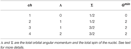
Table 1. List of the channels for a J^π = 1/2⁺ system.

In the present work, the hyperradial function is itself expanded on a suitable basis, i.e., a set of generalized Laguerre polynomials [1]. Therefore, we can write

$\begin{array}{ll}{u}_{\left\{G\right\}}(\rho )={\displaystyle \sum _l}{c}_{\left\{G\right\},l}{f}_l(\rho ),& (18)\end{array}$

where c_{{G}, l} are unknown coefficients, and

$\begin{array}{ll}{f}_l(\rho )=\sqrt{\frac{l!}{(l+5)!}}{\gamma }^3{}^{(5)}{L}_l(\gamma \rho )e^{-\frac{\gamma }{2}\rho }.& (19)\end{array}$

Here ${}^{(5)}{L}_l(\gamma \rho )$ are generalized Laguerre polynomials, and the numerical factor in front of them is chosen so that f_l(ρ) are normalized to unit. Furthermore, γ is a non-linear parameter, whose typical values are in the range (2 − 5) fm⁻¹. The results have to be stable against γ, as we will show in section 3. With these assumptions, the functions f_l(ρ) go to zero for ρ → ∞, and constitute an orthonormal basis.

By using Equation (18), the wave function can now be cast in the form

$\begin{array}{ll}\Psi ={\displaystyle \sum _{\left\{G\right\}}}{\displaystyle \sum _{l=1}^{N_{max}}}{c}_{\left\{G\right\},l}B{H}_{\left\{G\right\}}^J(\Omega )f_l(\rho ),& (20)\end{array}$

where we have dropped the superscript (3) in Ω⁽³⁾ to simplify the notation, and we have indicated with N_max the maximum number of Laguerre polynomials in Equation (18).

In an even more compact notation, we can write

$\begin{array}{ll}\Psi ={\displaystyle \sum _{\xi }}{c}_{\xi }{\Psi }_{\xi },& (21)\end{array}$

where Ψ_ξ is a complete set of states, and ξ is the index that labels all the quantum numbers defining the basis elements. The expansion coefficients c_ξ can be determined using the Rayleigh-Ritz variational principle [1], which states that

$\begin{array}{ll}\langle {\delta }_c\Psi |H-E|\Psi \rangle =0,& (22)\end{array}$

where δ_cΨ denotes the variation of the wave function with respect to the coefficients c_ξ. By doing the differentiation, the problem is then reduced to a generalized eigenvalue-eigenvector problem of the form

$\begin{array}{ll}{\displaystyle \sum _{{\xi }^{\prime }}}\langle {\Psi }_{\xi }|H-E|{\Psi }_{{\xi }^{\prime }}\rangle c_{{\xi }^{\prime }}=0,& (23)\end{array}$

that is solved using the Lanczos diagonalization algorithm [9]. The use of the Lanczos algorithm is dictated by the large size (~ 50000 × 50000) of the involved matrices (see below).

All the computational problem is now shifted in having to calculate the norm, kinetic energy and potential energy matrix elements. One of the advantage of using a fixed permutation is that the norm and kinetic energy matrix elements are or analytical, or involve just a one-dimensional integration. In fact, they are written as

$\begin{array}{ll}{N}_{\left\{G^{\prime }\right\},k;\left\{G\right\},l}\equiv \langle {\Psi }_{{\xi }^{\prime }}|{\Psi }_{\xi }\rangle =J{\delta }_{\xi ,{\xi }^{\prime }},& (24)\end{array}$

$\begin{array}{l}{T}_{\left\{G^{\prime }\right\},k;\left\{G\right\},l}\equiv \langle {\Psi }_{{\xi }^{\prime }}|T|{\Psi }_{\xi }\rangle =-\frac{{\hslash }^2}{2M}J{\delta }_{\left\{G\right\},\left\{G^{\prime }\right\}}{\displaystyle \int }d\rho {\rho }^5{f}_k(\rho )\\ \times \left[-G(G+4)\frac{f_l(\rho )}{{\rho }^2}+5\frac{f_l^{\prime }(\rho )}{\rho }+f_l^{″}(\rho )\right],& (25)\end{array}$

where J is the total Jacobian of the transformation, given by

$\begin{array}{ll}J={\left(M\sqrt{\frac{m_{tot}}{m_1{m}_2{m}_3}}\right)}^3,& (26)\end{array}$

and $f_l^{\prime }(\rho )$ and $f_l^{″}(\rho )$ are, respectively, the first and the second derivatives of the functions f_l(ρ) defined in Equation (19).

The potential matrix elements in Equation (23) can be written as

$\begin{array}{ll}{V}_{\left\{G^{\prime }\right\},k;\left\{G\right\},l}\equiv \langle {\Psi }_{{\xi }^{\prime }}|V_{12}+V_{23}+V_{13}|{\Psi }_{\xi }\rangle ,& (27)\end{array}$

with V_ij indicating the two-body interaction between particle i and particle j. Note that in the present work we do not consider three-body forces. Since it is easier to evaluate the matrix elements of V_ij when the Jacobi coordinate y₂ is proportional to r_i − r_j, we proceed as follows. We make use of the fact that the hyperradius is permutation-independent, and we use the fact that the HH function written in terms of Ω^(p) can be expressed as function of the HH written using Ω^(p′), with p′ ≠ p. Basically it can be shown that [1]

$\begin{array}{ll}{H}_{[G]}({\Omega }^{(p)})={\displaystyle \sum _{[G^{\prime }]}}{a}_{[G],[G^{\prime }]}^{(p\to p^{\prime }),G,\Lambda }{H}_{[G^{\prime }]}({\Omega }^{(p^{\prime })}),& (28)\end{array}$

where the grandangular momentum G and the total angular momentum Λ remain constant, i.e., G = G′ and Λ = Λ′, but we have [G] ≠ [G′], since all possible combinations of ℓ₁, ℓ₂, n are allowed. The spin-part written in terms of permutation p can be easily expressed in terms of permutation p′ via the standard 6j Wigner coefficients [10]. The transformation coefficients $a_{\left[G\right],\left[G^{\prime }\right]}^{(p\to p^{\prime }),G}$ can be calculated, for A = 3, through the Raynal-Revai recurrence relations [11]. Alternately we can use the orthonormality of the HH basis [1], i.e.,

$\begin{array}{ll}{a}_{[G],[G^{\prime }]}^{(p\to p^{\prime }),G,\Lambda }={\displaystyle \int }d{\Omega }^{(p^{\prime })}{[H_{[G^{\prime }]}({\Omega }^{(p^{\prime })})]}^{†}{H}_{[G]}({\Omega }^{(p)}).& (29)\end{array}$

Their explicit expression can be found for instance in Kievsky et al. [1] as is reported in the Appendix for completeness. The final expression for the potential matrix elements is given by

$\begin{array}{l}\langle {\Psi }_{{\xi }^{\prime }}|V_{12}+V_{23}+V_{13}|{\Psi }_{\xi }\rangle =J{\displaystyle \int }d\rho {\rho }^5{f}_k(\rho )f_l(\rho )\\ \times \{{\displaystyle \int }d{\Omega }^{(3)}B{H}_{{\xi }^{\prime }}^{†}({\Omega }^{(3)})V_{12}B{H}_{\xi }({\Omega }^{(3)})\\ +{\displaystyle \sum _{{\xi }^{″}}}{\displaystyle \sum _{{\xi }^{‴}}}[a_{{\xi }^{\prime }\to {\xi }^{‴}}^{(3\to 1),G^{\prime },{\Lambda }^{\prime }}{a}_{\xi \to {\xi }^{″}}^{(3\to 1),G,\Lambda }\\ \times {\displaystyle \int }d{\Omega }^{(1)}B{H}_{{\xi }^{‴}}^{†}({\Omega }^{(1)})V_{23}B{H}_{{\xi }^{″}}({\Omega }^{(1)})\\ +a_{{\xi }^{\prime }\to {\xi }^{‴}}^{(3\to 2),G^{\prime },{\Lambda }^{\prime }}{a}_{\xi \to {\xi }^{″}}^{(3\to 2),G,\Lambda }\\ \times {\displaystyle \int }d{\Omega }^{(2)}B{H}_{{\xi }^{‴}}^{†}({\Omega }^{(2)})V_{13}B{H}_{{\xi }^{″}}({\Omega }^{(2)}]\}.& (30)\end{array}$

It is then clear the advantage of using the NSHH method also for the calculation of the potential matrix elements, as in fact all what is needed is the calculation of one integral of the type

$\begin{array}{ll}I(\rho )={\displaystyle \int }d\rho {\rho }^5{f}_k(\rho )f_l(\rho ){\displaystyle \int }d{\Omega }^{(p)}B{H}_{{\xi }^{‴}}^{†}({\Omega }^{(p)})V_{ij}B{H}_{{\xi }^{″}}({\Omega }^{(p)}),& (31)\end{array}$

with p the permutation corresponding to the order i, j, k.

3. Results

We present in this section the results obtained with the NSHH method described above. In particular, we present in section 3.1 the study of the convergence of the method, in the case of the triton binding energy, calculated with m_p = m_n. We then present in section 3.2 the results for the triton and ³He binding energy, when m_p ≠ m_n. In section 3.3 we present the results of the hypertriton.

The potential models used in our study are central spin-independent and spin-dependent. In particular, the ³H and ³He systems have been investigated using the spin-independent Volkov [12], Afnan-Tang [13], and Malfliet-Tjon [14] potential models, and the two spin-dependent Minnesota [15] and Argonne AV4′ [16] potential models. Note that the AV4′ potential is a reprojection of the much more realistic Argonne AV18 [17] potential model. In the case of the hypernucleus ${}_{\Lambda }{}^3\text{H}$, we have used the Gaussian spin-independent central potential of Clare and Levinger [18], and two spin-dependent potentials: the first one, labeled MN9 [19], combines a Minnesota [15] potential for the NN interaction with the S = 1 component of the same Minnesota potential multiplied by a factor 0.9 for the ΛN interaction. The second one, labeled AU, uses the Argonne AV4′ of Wiringa and Pieper [16] for the NN interaction, and the Usmani potential of Usmani and Khanna [20] for the ΛN interaction (see also Ferrari Ruffino et al. [21]).

3.1. Convergence Study

We recall that the wave function is written as in Equation (20), and that, since we are using central potentials, only the first channel of Table 1 is considered, as for instance in Kievsky et al. [1]. Therefore we need to study the convergence of our results on G^max and N_max. Furthermore, we introduce the value of j as $\overrightarrow{j}={\overrightarrow{\ell }}_2+\overrightarrow{S}$, ℓ₂ and S being the orbital angular momentum and the spin of the pair ij on which the potential acts. This allows to set up the theoretical framework also in the case of projecting potentials. Therefore, we will study the convergence of our results also on the maximum value of j, called j_max. Finally, the radial function written as in Equation (19), presents a non-linear parameter γ, for which we need to find a range of values such that the binding energy is stable. Note that in these convergence studies we have used m_n = m_p.

We start by considering the parameter γ. The behavior of the binding energy as a function of γ is shown for the Volkov potential in the top panel of Figure 1. We mention here that for all the other potential models we have considered, the results are similar. The other parameters were kept constant, i.e., G^max = 20, N_max = 16, and j_max = 6. The particular dependence on γ of the binding energy, that increases for low values of γ, is constant for some central values, and decreases again for large values of γ, allows to determine a so-called plateau, and the optimal value for γ has to be chosen on this plateau. Alternatively, we can chose γ such that for a given N_max the binding energy is maximum. A choice of γ outside the plateau would require just a larger value of N_max. To be noticed that this particular choice of γ is not universal. As an example, in the “standard” HH method, γ = 2.5 − 4.5 fm⁻¹ for the AV18 potential, but much larger (≃ 7 fm⁻¹) for the chiral non-local potentials [1]. In our case, different values of γ for different potentials might improve the convergence on N_max, but not that on j_max and G^max, determined by the structure of the HH functions. Since, as shown below, the convergence on N_max is not difficult to be achieved, we have chosen to keep γ at a fixed value, i.e., γ = 4 fm⁻¹ for all the potentials.

FIGURE 1

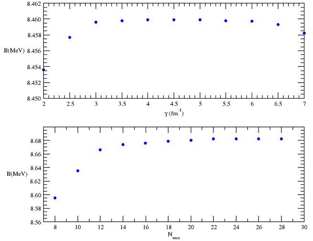
Figure 1. (Top) The binding energy B (in MeV) as function of the parameter14 γ (in fm⁻¹) for the Volkov potential model [12], with G^max = 20, j_max = 6 and N_max = 16, and using m_n = m_p. (Bottom) The binding energy B (in MeV) as function of the parameter N_max for the AV4′ potential model [16], with G^max = 20, j_max = 8 and γ = 4 fm⁻¹, and using m_n = m_p.

In the bottom panel of Figure 1 we fix j_max = 8, γ = 4 fm⁻¹, and G^max = 20, and we show the pattern of convergence for the binding energy B with respect to N_max, in the case of the Argonne AV4′ model. Here convergence is reached for N_max = 24, i.e., we have verified that, for higher N_max value, B changes by less than 1 keV. To be noticed that for the other potentials, convergence is already reached for N_max = 16 − 20.

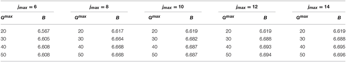
The variation of the binding energy as a function of j_max and G^max depends significantly on the adopted potential model. Therefore, we need to analyze every single case. As we can see from the data of Tables 2 and 3, the convergence on j_max and G^max for the Volkov and the Minnesota potentials is really quick, and we can reach an accuracy better than 2 keV for j_max = 10 and G^max = 40. On the other hand, in the case of the Afnan-Tang potential, we need to go up to j_max = 14 and G^max = 50, in order to get a total accuracy of our results of about 2 keV (1 keV is due to the dependence on N_max). This can be seen by inspection of Table 4. The Malfliet-Tjon potential model implies a convergence even slower of the expansion, and we have to go up to G^max = 90 and j_max = 22, to get an uncertainty of about 3 keV, as shown in Table 5. In fact, being a sum of Yukawa functions, the Malfliet-Tjon potential model is quite difficult to be treated also with the “standard” symmetrized HH method [1].

TABLE 2

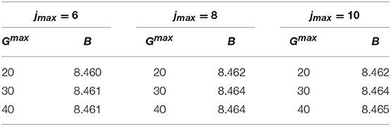
Table 2. The ³H binding energy B (in MeV) calculated with the Volkov potential model [12], using m_n = m_p, N_max = 16, and γ = 4 fm⁻¹, as function of j_max and G^max.

TABLE 3

Table 3. Same as Table 2 but for the Minnesota potential model [15].

TABLE 4

Table 4. Same as Table 2 but for the Afnan-Tang potential model [13].

TABLE 5

Table 5. Same as Table 2 but for the Malfliet-Tjon potential model [14].

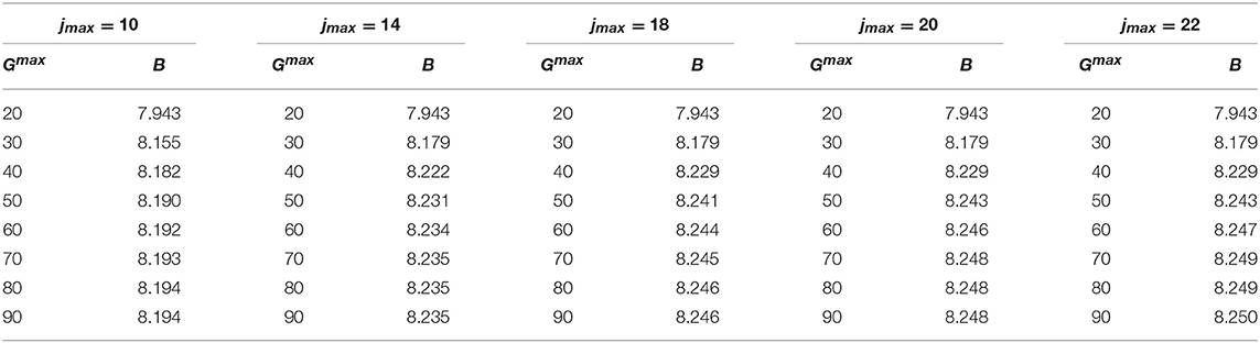
In Tables 6 and 7, we show the convergence study for the AV4′, which is the most realistic potential model used here for the A = 3 nuclear systems. As we can see by inspection of the tables, in order to reach an accuracy of about 3 keV, we have to push the calculation up to G^max = 80, N_max = 24, and j_max = 20. Our final result of B = 8.991 MeV, though, agrees well with the one of Marcucci¹, obtained with the “standard” symmetrized HH method, for which B = 8.992 MeV.

TABLE 6

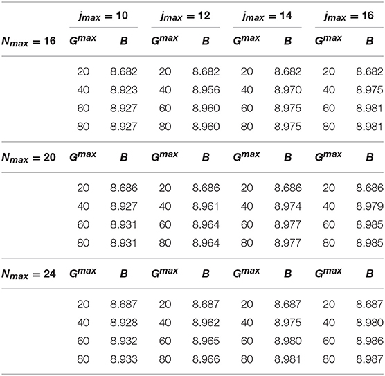
Table 6. The ³H binding energy B (in MeV) calculated with the AV4′ potential model [16] as function of N_max, j_max, and G^max, using m_n = m_p and γ = 4 fm⁻¹.

TABLE 7

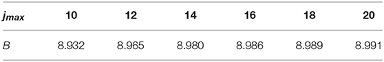
Table 7. The ³H binding energy B (in MeV) calculated with the AV4′ potential model [16], using m_n = m_p, G^max = 60, N_max = 24 ,and γ = 4 fm⁻¹.

The results for the binding energy of ³H and ³He with the different potentials will be summarized in the next subsection.

3.2. The ³H and ³He Systems

Having verified that our method can be pushed up to convergence, we present in the third column of Table 8 the results for the ³H binding energy with all the different potential models, obtained still keeping m_p = m_n. The results are compared with those present in the literature, finding an overall nice agreement.

TABLE 8

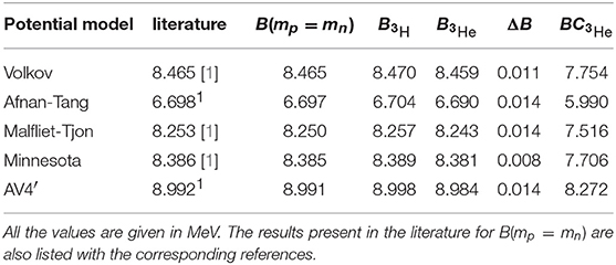
Table 8. The ³H binding energy obtained using m_n = m_p (B(m_p = m_n)), the ³H and ³He binding energies calculated taking into account the difference of masses but no Coulomb interaction in ³He ($B_{{}^3\text{H}}$ and $B_{{}^3\text{He}}$), the difference $\Delta B=B_{{}^3\text{H}}-B_{{}^3\text{He}}$, and the ³He binding energy calculated including also the (point) Coulomb interaction ($B{C}_{{}^3\text{He}}$).

We now turn our attention to the ³H and ³He nuclei, considering them as made of different mass particles. Therefore, we impose m_p ≠ m_n and we calculate the ³H and ³He binding energy and the difference of these binding energies, i.e.,

$\begin{array}{ll}\Delta B=B_{{}^3\text{H}}-B_{{}^3\text{He}}.& (32)\end{array}$

To be noticed that we have not yet included the effect of the (point) Coulomb interaction. The results are listed in Table 8. By inspection of the table, we can see that ΔB is not the same for all the potential models. In fact, while for the spin-independent Afnan-Tang and Malfliet-Tjon central potentials, and for the spin-dependent AV4′ potential, ΔB = 14 keV, for the Volkov and the Minnesota potential we find a smaller value. In all cases, though, we have verified that ΔB is equally distributed, i.e., we have verified that

$\begin{array}{ll}{B}_{m_n=m_p}=B_{{}^3\text{H}}-\frac{\Delta B}{2}=B_{{}^3\text{He}}+\frac{\Delta B}{2},& (33)\end{array}$

as can be seen from Table 8. We would like to remark that in the NSHH method, the inclusion of the difference of masses is quite straightforward, and ΔB can be calculated “exactly.” This is not so trivial within the symmetrized HH method. Furthermore, we compare our results with those of Nogga et al. [22], where ΔB was calculated within the Faddeev equation method using realistic Argonne AV18 [17] potential, and it was found ΔB = 14 keV, in perfect agreement with our AV4′ result.

In order to test our results for ΔB, we try to get a perturbative rough estimate of ΔB, proceeding as follows: since the neutron-proton difference of mass Δm = m_n − m_p = 1.2934 MeV is about three orders of magnitude smaller than their average mass m = (m_n + m_p)/2 = 938.9187 MeV, we can assume also ΔB to be small. Furthermore, we suppose the potential to be insensitive to Δm, and we consider only the kinetic energy. In the center of mass frame, the kinetic energy operator can be cast in the form

$\begin{array}{ll}T={\displaystyle \sum _{i=1}^3}\frac{{\text{p}}_i^2}{2m_i}=\frac{{\text{p}}_1^2+{\text{p}}_2^2}{2m_e}+\frac{{\text{p}}_3^2}{2m_d},& (34)\end{array}$

where m_e stands for the mass of the two equal particles, i.e., m_n for ³H and m_p for ³He, and m_d is the mass of the third particle, different from the previous ones. By defining E = 〈H〉 = 〈T + V〉, where 〈H〉 is the average value of the Hamiltonian H, we obtain

$\begin{array}{ll}\frac{\partial E}{\partial m_e}=\langle \frac{\partial H}{\partial m_e}\rangle =\langle \frac{\partial T}{\partial m_e}\rangle =-\frac{\langle 2T_e\rangle }{m_e},& (35)\end{array}$

$\begin{array}{ll}\frac{\partial E}{\partial m_d}=\langle \frac{\partial H}{\partial m_d}\rangle =\langle \frac{\partial T}{\partial m_d}\rangle =-\frac{\langle T_d\rangle }{m_d},& (36)\end{array}$

where we have indicated $\langle T_{e/d}\rangle \approx {\text{p}}_i^2/(2m_{e/d})$. Moreover, we define the proton and neutron mass difference Δm_p/n as

$\begin{array}{ll}\Delta m_p\equiv m_p-m=-\frac{\Delta m}{2},& (37)\end{array}$

$\begin{array}{ll}\Delta m_n\equiv m_n-m=\frac{\Delta m}{2},& (38)\end{array}$

and the ³He and ³H binding energy difference $\Delta B_{{}^3\mathrm{\text{He}}{/}^3\mathrm{\text{H}}}$ as

$\begin{array}{ll}\Delta B_{{}^3\text{He}}\equiv B_{m_n=m_p}-B_{{}^3\text{He}},& (39)\end{array}$

$\begin{array}{ll}\Delta B_{{}^3\text{H}}=B_{m_n=m_p}-B_{{}^3\text{H}}.& (40)\end{array}$

Then using Equations (35)–(38), we obtain

$\begin{array}{l}\Delta B_{{}^3\text{He}}\approx \frac{\partial E}{\partial m_e}\Delta m_p+\frac{\partial E}{\partial m_d}\Delta m_n=\frac{\langle 2T_e\rangle }{m_e}\frac{\Delta m}{2}-\frac{\langle T_d\rangle }{m_d}\frac{\Delta m}{2}\\ \approx \langle 2T_e-T_d\rangle \frac{\Delta m}{2m}.& (41)\end{array}$

$\begin{array}{l}\Delta B_{{}^3\text{H}}\approx \frac{\partial E}{\partial m_e}\Delta m_n+\frac{\partial E}{\partial m_d}\Delta m_p=-\frac{\langle 2T_e\rangle }{m_e}\frac{\Delta m}{2}+\frac{\langle T_d\rangle }{m_d}\frac{\Delta m}{2}\\ \approx -\langle 2T_e-T_d\rangle \frac{\Delta m}{2m}.& (42)\end{array}$

In conclusion

$\begin{array}{ll}\Delta B_{PT}\equiv B_{{}^3\text{H}}-B_{{}^3\text{He}}\approx \langle 2T_e-T_d\rangle \frac{\Delta m}{m}\approx \langle T\rangle \frac{\Delta m}{3m},& (43)\end{array}$

where the last equality holds assuming that 〈T_e〉 = 〈T_d〉 = 〈T〉/3, since the ³He and ³H have a large S-wave component (about 90 %). The results of 〈T〉 and ΔB_PT are listed in Table 9, and are compared with the values for ΔB calculated within the NSHH and already listed in Table 8. By inspection of the table we can see an overall nice agreement between this rough estimate and the exact calculation for all the potential models. Only in the case of the Minnesota and AV4′ potentials, ΔB_PT is 4 and 3 keV larger than ΔB, respectively. This can be understood by noticing that these potentials are spin-dependent, giving rise to mixed-symmetry components in the wave functions. These components are responsible for a reduction in ΔB_PT [23], related to the fact that the nuclear force for the ³S₁ np pair is stronger than for the ¹S₀ nn (or pp) pair. Therefore, the kinetic energy for equal particles 〈T_e〉 is less than the kinetic energy for different particles 〈T_d〉.

TABLE 9

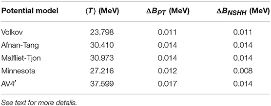
Table 9. Mean value for the kinetic energy operator 〈T〉, ΔB estimated with the perturbative theory (PT), and ΔB calculated with the NSHH for the different potential models considered in this work.

3.3. The ${}_{\Lambda }{}^3\text{H}$ Hypernucleus

The hypernucleus ${}_{\Lambda }{}^3\text{H}$ is a bound system composed by a neutron, a proton, and the Λ hyperon. In order to study this system, we have considered the proton and the neutron as reference-pair, with equal mass m_n = m_p = m, while the Λ particle has been taken as the third particle with different mass. The Λ hyperon mass has been chosen depending on the considered potential. We remind that we have used three different potential models: a central spin-independent Gaussian model [18], and two spin-dependent central potentials, labeled MN9 [19] and AU [21] potentials. Therefore, when the ${}_{\Lambda }{}^3\text{H}$ hypernucleus has been studied using the Gaussian potential of Clare and Levinger [18], we have set M_Λ = 6/5 m_N, accordingly. In the other two cases, we have used M_Λ = 1115.683 MeV. We first study the convergence pattern of our method, which in the case of the Gaussian potential of Clare and Levinger [18] is really fast, with a reached accuracy of 1 keV on the binding energy already with N_max = 20, j_max = 10, and G^max = 50. This can be seen directly by inspection of Tables 10 and 11.

TABLE 10

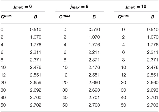
Table 10. The ${}_{\Lambda }{}^3\text{H}$ binding energy B (in MeV) as function of j_max and G^max, calculated with the Gaussian potential model of Clare and Levinger [18], using N_max = 20, and γ = 4 fm⁻¹.

TABLE 11

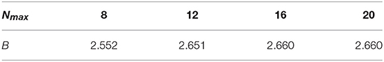
Table 11. The ${}_{\Lambda }{}^3\text{H}$ binding energy B (in MeV) as function of N_max, calculated with the the Gaussian potential model of Clare and Levinger [18], using G^max = 20, j_max = 8, and γ = 4 fm⁻¹.

The convergence pattern in the case of the spin-dependent central MN9 and AU potentials has been found quite slower. This is shown in Tables 12 and 13, respectively. By inspection of Table 12, we can conclude that B = 2.280 MeV, with an accuracy of about 3 keV, obtained with G^max = 100, N_max = 34, and j_max = 14. By inspection of Table 13, B = 2.532 MeV, with an accuracy of about 4 keV, going up to G^max = 140, N_max = 24, and j_max = 16.

TABLE 12

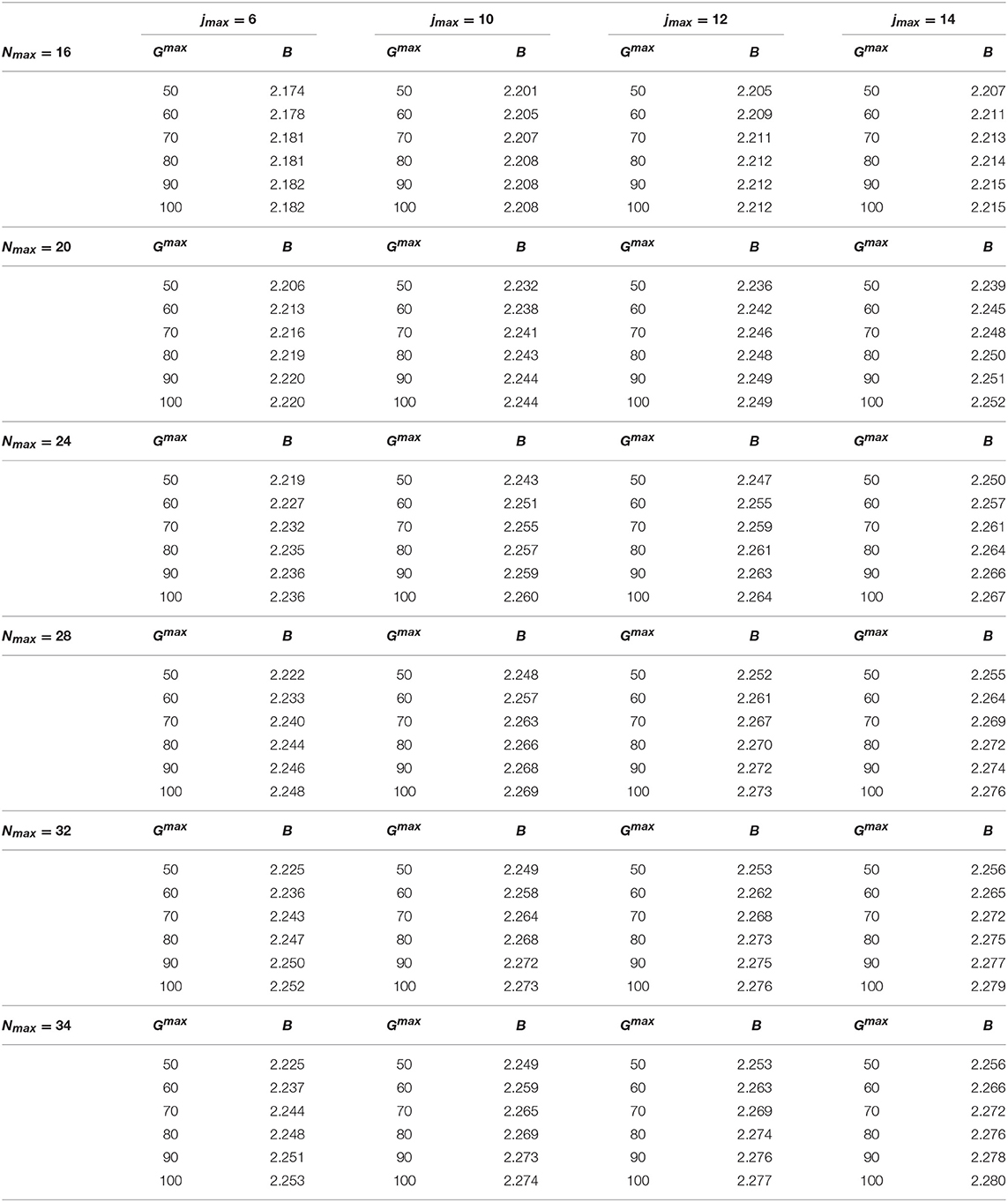
Table 12. The ${}_{\Lambda }{}^3\text{H}$ binding energy B (in MeV) as function of G^max, j_max, and N_max, calculated with the MN9 potential model of Ferrari Ruffino [19], using γ = 4 fm⁻¹.

TABLE 13

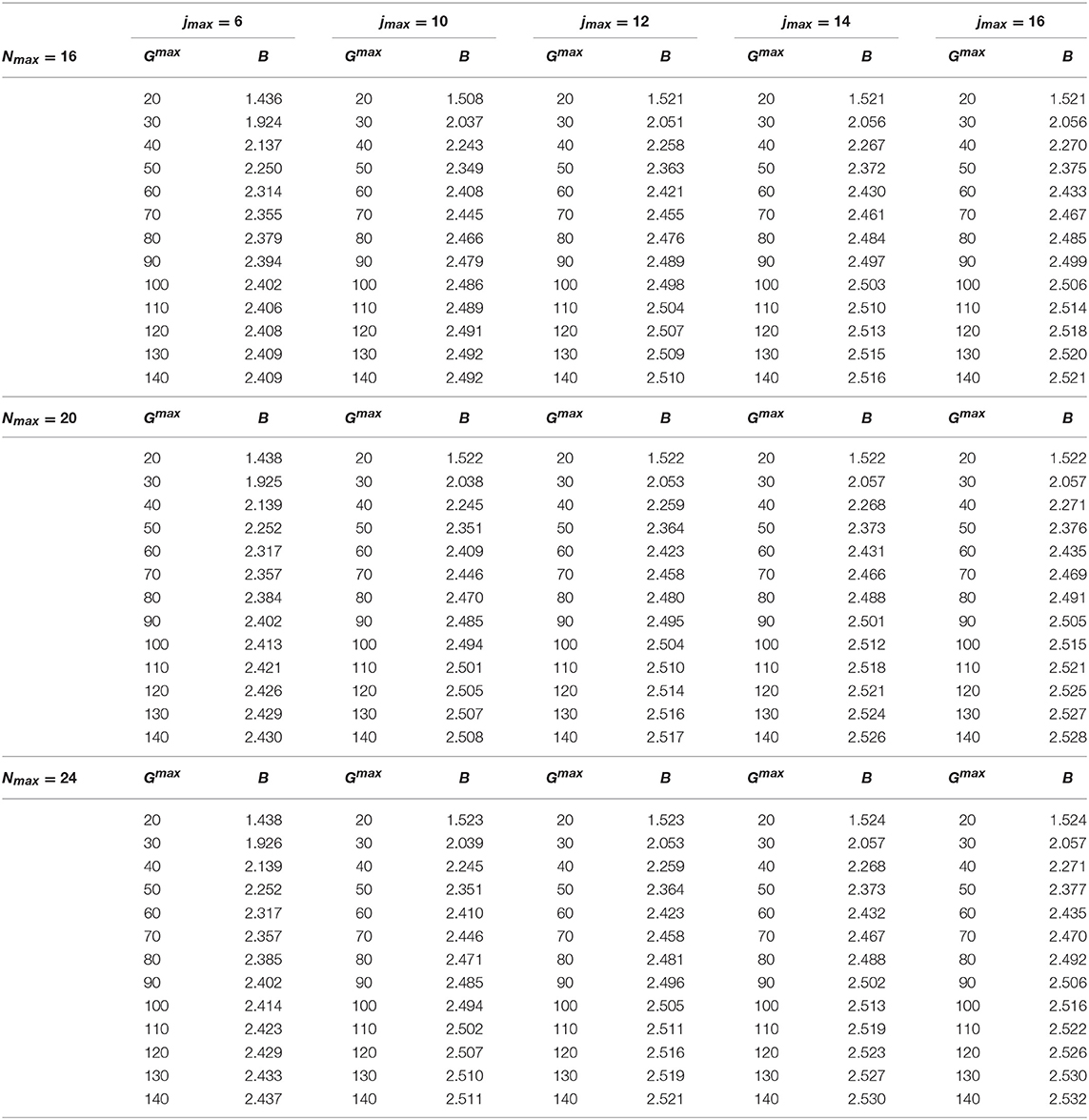
Table 13. Same as Table 12 but using the AU potential model of Ferrari Ruffino et al. [21] for N_max = 16, 20, 24.

The results obtained with our method for the three potential models considered in this work are compared with those present in the literature [18, 19, 21] in Table 14, finding a very nice agreement, within the reached accuracy.

TABLE 14

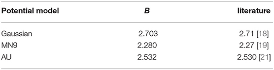
Table 14. The ${}_{\Lambda }{}^3\text{H}$ binding energy B (in MeV) obtained in the present work is compared with the results present in the literature.

4. Conclusions and Outlook

In this work we present a study of the bound state of a three-body system, composed of different particles, by means of the NSHH method. The method has been reviewed in section 2. In order to verify its validity, we have started by considering a system of three equal-mass nucleons interacting via different central potential models, three spin-independent and two spin-dependent. We have studied the convergence pattern, and we have compared our results at convergence with those present in the literature, finding an overall nice agreement. Then, we have switched on the difference of mass between protons and neutrons and we have calculated the difference of binding energy ΔB due to the difference between the neutron and proton masses. We have found that ΔB depends on the considered potential model, but is always symmetrically distributed (see Equation (33)).

Finally we have implemented our method for the ${}_{\Lambda }{}^3\text{H}$ hypernucleus, studied with three different potentials, i.e., the Gaussian potential of Clare and Levinger [18], for which we have found a fast convergence of the NSHH method, the MN9 and the AU potentials of Ferrari Ruffino [19], for which the convergence is much slower. In these last two cases, in particular, we had found necessary to include a large number of the HH basis (46104 for the MN9 and 52704 for the AU potentials), but the agreement with the results in the literature has been found quite nice. To be noticed that we have included only two-body interactions, and therefore a comparison with the experimental data is meaningless.

In conclusion, we believe that we have proven the NSHH method to be a good choice for studying three-body systems composed of two equal mass particles, different from the mass of the third particle. Besides ³H, ³He, and ${}_{\Lambda }{}^3\text{H}$, several other nuclear systems can be viewed as three-body systems of different masses. This applies in all cases where a strong clusterization is present, as in the case of ⁶He and ⁶Li nuclei, seen as NNα , or the ⁹Be and ⁹B, seen as a ααN three-body systems. Furthermore, taking advantage of the versatility of the HH method also for scattering systems, the NSHH approach could be extended as well to scattering problems. Work along these lines are currently underway.

Author Contributions

In this work, the theoretical formalism has been derived independently by both authors. The needed computer codes have been developed essentially by AN, starting from the work of LEM, and have been checked independently by LEM. The manuscript is the result of an even effort of both authors.

Conflict of Interest Statement

The authors declare that the research was conducted in the absence of any commercial or financial relationships that could be construed as a potential conflict of interest.

Acknowledgments

The authors would like to thank Dr. F. Ferrari Ruffino for useful discussions. Computational resources provided by the INFN-Pisa Computer Center are gratefully acknowledged.

Footnotes

1. ^Marcucci LE. Private Communication. (2018).

References

1. Kievsky A, Rosati S, Viviani M, Marcucci LE, Girlanda L. A High-precision variational approach to three- and four-nucleon bound and zero-energy scattering states. J Phys G (2008) 35:063101. doi: 10.1088/0954-3899/35/6/063101

CrossRef Full Text | Google Scholar

2. Leidemann W, Orlandini G. Modern ab initio approaches and applications in few-nucleon physics with A ≥ 4. Prog Part Nucl Phys. (2013) 68:158. doi: 10.1016/j.ppnp.2012.09.001

CrossRef Full Text | Google Scholar

3. Gattobigio M, Kievsky A, Viviani M, Barletta P. The Harmonic hyperspherical basis for identical particles without permutational symmetry. Phys Rev. (2009) A79:032513. doi: 10.1103/PhysRevA.79.032513

CrossRef Full Text | Google Scholar

4. Gattobigio M, Kievsky A, Viviani M, Barletta P. Non-symmetrized Basis Function for Identical Particles. Few Body Syst. (2009) 45:127. doi: 10.1007/s00601-009-0045-4

CrossRef Full Text | Google Scholar

5. Gattobigio M, Kievsky A, Viviani M. Non-symmetrized hyperspherical harmonic basis for A-bodies. Phys Rev. (2011) C83:024001. doi: 10.1103/PhysRevC.83.024001

CrossRef Full Text | Google Scholar

6. Deflorian S, Barnea N, Leidemann W, Orlandini G. Nonsymmetrized hyperspherical harmonics with realistic NN potentials. Few Body Syst. (2013) 54:1879. doi: 10.1007/s00601-013-0717-y

CrossRef Full Text | Google Scholar

7. Deflorian S, Barnea N, Leidemann W, Orlandini G. Nonsymmetrized hyperspherical harmonics with realistic potentials. Few-Body Syst. (2014) 55:831. doi: 10.1007/s00601-013-0781-3

CrossRef Full Text | Google Scholar

8. Rosati S. The hyperspherical harmonics method: a review and some recent developments. In: Fabrocini A, Fantoni S, Krotscheck E, editors. Introduction to Modern Methods of Quantum Many-Body Theory and Their Applications, Series on Advances in Quantum Many-Body Theory, vol.7. London; Singapore; Hong Kong: World Scientific (2002). p. 339.

Google Scholar

9. Chen CR, Payne GL, Friar JL, Gibson BF. Faddeev calculations of the 2π-3N force contribution to the ³H binding energy. Phys Rev C (1986) 33:1740. doi: 10.1103/PhysRevC.33.1740

CrossRef Full Text | Google Scholar

10. Edmonds AR. Angular Momentum in Quantum Mechanics. Princeton, NJ: Princeton University Press (1974).

Google Scholar

11. Raynal J, Revai J. Transformation coefficients in the hyperspherical approach to the three-body problem. Il Nuovo Cimento A (1970) 68:612. doi: 10.1007/BF02756127

CrossRef Full Text | Google Scholar

12. Volkov AB. Equilibrium deformation calculations of the ground state energies of 1p shell nuclei. Nucl Phys. (1965) 74:33.

Google Scholar

13. Afnan IR, Tang YC. Investigation of nuclear three- and four-body systems with soft-core nucleon-nucleon potentials. Phys Rev. (1968) 175:1337.

Google Scholar

14. Malfliet RA, Tjon JA. Three nucleon calculations with local tensor forces. Phys Lett B (1969) 30:293.

Google Scholar

15. Thompson DR, Lemere M, Tang YC. Systematic investigation of scattering problems with the resonating-group method. Nucl Phys A (1977) 286:53.

Google Scholar

16. Wiringa RB, Pieper SC. Evolution of nuclear spectra with nuclear forces. Phys Rev Lett. (2002)89:182501. doi: 10.1103/PhysRevLett.89.182501

PubMed Abstract | CrossRef Full Text | Google Scholar

17. Wiringa RB, Stoks VGJ, Schiavilla R. Accurate nucleon-nucleon potential with charge-independence breaking. Phys Rev C (1995) 51:38. doi: 10.1103/PhysRevC.51.38

PubMed Abstract | CrossRef Full Text | Google Scholar

18. Clare RB, Levinger JS. Hypertriton and hyperspherical harmonics. Phys Rev C (1985) 31:2303. doi: 10.1103/PhysRevC.31.2303

PubMed Abstract | CrossRef Full Text | Google Scholar

19. Ferrari Ruffino F. Non-Symmetrized Hyperspherical Harmonics Method Applied to Light Hypernuclei. PhD Thesis, University of Trento, Trento (2017).

20. Usmani AA, Khanna FC. Behaviour of the ΛN and ΛNN potential strengths in the ${}_{\Lambda }{}^5\text{He}$ hypernucleus. J Phys G (2008) 35:025105. doi: 10.1088/0954-3899/35/2/025105

CrossRef Full Text | Google Scholar

21. Ferrari Ruffino F, Barnea N, Deflorian S, Leidemann W, Lonardoni D, Orlandini G, et al. Benchmark Results for Few-Body Hypernuclei. Few Body Syst. (2017) 58:113. doi: 10.1007/s00601-017-1273-7

CrossRef Full Text | Google Scholar

22. Nogga A, Kievsky A, Kamada H, Glöckle W, Marcucci LE, Rosati S, et al. Three-nucleon bound states using realistic potential models. Phys Rev C (2003) 67:034004. doi: 10.1103/PhysRevC.67.034004

CrossRef Full Text | Google Scholar

23. Friar JL, Gibson BF, Payne GL. n − p mass difference and charge-symmetry breaking in the trinucleons. Phys Rev C. (1990) 42:1211.

PubMed Abstract | Google Scholar

Appendix: The Transformation Coefficients

Let us start by writing Equation (29) as

$\begin{array}{l}{a}_{{\ell }_1,{\ell }_2,n,{\ell }_1^{\prime },{\ell }_2^{\prime },n^{\prime }}^{(p\to p^{\prime }),G,\Lambda }={\displaystyle \int }d{\Omega }^{(p^{\prime })}{[H_{[{\ell }_1^{\prime },{\ell }_2^{\prime },n^{\prime },\Lambda {\Lambda }_z]}({\Omega }^{(p^{\prime })})]}^{†}\\ H_{\left[{\ell }_1,{\ell }_2,n,\Lambda {\Lambda }_z\right]}({\Omega }^{(p)}),& (\text{A}1)\end{array}$

where ℓ_i (${\ell }_i^{\prime }$) is the orbital angular momentum associated with the Jacobi coordinate ${\mathbf{\text{y}}}_i^{(p)}$ (${\mathbf{\text{y}}}_i^{(p^{\prime })}$). It can be demonstrated by direct calculation and exploiting the spherical harmonics proprieties that

$\begin{array}{l}{a}_{{\ell }_1,{\ell }_2,n,{\ell }_1^{\prime },{\ell }_2^{\prime },n^{\prime }}^{(p\to p^{\prime }),G,L}=N_{n^{\prime }}^{{\ell }_1^{\prime },{\ell }_2^{\prime }}{N}_n^{{\ell }_1,{\ell }_2}\frac{1}{2}{\displaystyle {\int }_0^{\frac{\pi }{2}}}d\varphi {\displaystyle {\int }_{-1}^1}d\mu {(cos{\varphi }^{(p^{\prime })})}^{2+{\ell }_2^{\prime }}{(sin{\varphi }^{(p^{\prime })})}^{2+{\ell }_1^{\prime }}\\ \times P_{n^{\prime }}^{{\ell }_1^{\prime }+1/2,{\ell }_2^{\prime }+1/2}(cos{2\varphi }^{(p^{\prime })})P_n^{{\ell }_1+1/2,{\ell }_2+1/2}(cos{2\varphi }^{(p)})\\ \times {\displaystyle \sum _{\lambda ,{\lambda }_1,{\lambda }_2}}{C}_{{\ell }_1,{\ell }_2,{\lambda }_1,{\lambda }_2}^{(p),(p^{\prime })}(sin{\varphi }^{(p^{\prime })},cos{\varphi }^{(p^{\prime })})P_{\lambda }(\mu )\\ \times {(-)}^{\Lambda +{\lambda }_2+{\ell }_2^{\prime }}(2\lambda +1){\widehat{{\ell }^{\prime }}}_1{\widehat{{\ell }^{\prime }}}_2{\widehat{\lambda }}_1{\widehat{\lambda }}_2\\ \times \left\{\begin{array}{ccc}{\ell }_1^{\prime }& {\ell }_2^{\prime }& \Lambda \\ {\lambda }_2& {\lambda }_1& \lambda \\ \end{array}\right\}\left(\begin{array}{ccc}{\ell }_1^{\prime }& {\lambda }_1& \lambda \\ 0& 0& 0\\ \end{array}\right)\left(\begin{array}{ccc}{\ell }_2^{\prime }& {\lambda }_2& \lambda \\ 0& 0& 0\end{array}\right).& (\text{A}2)\end{array}$

Here the curly brackets indicate the 6j Wigner coefficients, and the coefficients $C_{{\ell }_1,{\ell }_2,{\ell }_1^{\prime },{\ell }_2^{\prime }}^{(p),(p^{\prime })}(sin{\varphi }^{(p^{\prime })},cos{\varphi }^{(p^{\prime })})$ are defined as

$\begin{array}{l}{C}_{{\ell }_1,{\ell }_2,{\ell }_1^{\prime },{\ell }_2^{\prime }}^{(p),(p^{\prime })}(sin{\varphi }^{(p^{\prime })},cos{\varphi }^{(p^{\prime })})\\ ={\displaystyle \sum _{{\lambda }_1+{\lambda }_2={\ell }_1}}{\displaystyle \sum _{{\lambda }_1^{\prime }+{\lambda }_2^{\prime }={\ell }_2}}{(sin{\varphi }^{(p^{\prime })})}^{{\lambda }_1+{\lambda }_1^{\prime }}{(cos{\varphi }^{(p^{\prime })})}^{{\lambda }_2+{\lambda }_2^{\prime }}\\ \times {({\alpha }_{11(p^{\prime })}^{(p)})}^{{\lambda }_1}{({\alpha }_{12(p^{\prime })}^{(p)})}^{{\lambda }_2}{({\alpha }_{21(p^{\prime })}^{(p)})}^{{\lambda }_1^{\prime }}{({\alpha }_{22(p^{\prime })}^{(p)})}^{{\lambda }_2^{\prime }}\\ \times {(-)}^{{\lambda }_1+{\lambda }_2+{\lambda }_1^{\prime }+{\lambda }_2^{\prime }}{D}_{{\ell }_1,{\lambda }_1,{\lambda }_2}{D}_{{\ell }_2,{\lambda }_1^{\prime },{\lambda }_2^{\prime }}\\ \times \widehat{{\ell }_1}\widehat{{\ell }_2}\widehat{{\ell }_1^{\prime }}\widehat{{\ell }_2^{\prime }}{\widehat{\lambda }}_1{\widehat{\lambda }}_2{\widehat{\lambda }}_1^{\prime }{\widehat{\lambda }}_2^{\prime }\left(\begin{array}{ccc}{\lambda }_1& {\lambda }_1^{\prime }& {\ell }_1^{\prime }\\ 0& 0& 0\end{array}\right)\\ \times \left(\begin{array}{ccc}{\lambda }_2& {\lambda }_2^{\prime }& {\ell }_2^{\prime }\\ 0& 0& 0\end{array}\right)\left\{\begin{array}{ccc}{\lambda }_1& {\lambda }_2& {\ell }_1\\ {\lambda }_1^{\prime }& {\lambda }_2^{\prime }& {\ell }_2\\ {\ell }_1^{\prime }& {\ell }_2^{\prime }& \Lambda \end{array}\right\}.& (\text{A}3)\end{array}$

In Equation (3) $\widehat{\ell }\equiv \sqrt{2\ell +1}$, and the round (curly) brackets denote 3j (9j) Wigner coefficients. The coefficients ${\alpha }_{ij(p^{\prime })}^{(p)}$, with ij = 1, 2 are given by

$\begin{array}{ll}{\text{y}}_i^{(p)}={\displaystyle \sum _{j=1}^2}{\alpha }_{ij(p^{\prime })}^{(p)}{\text{y}}_j^{(p^{\prime })},& (\text{A}4)\end{array}$

and depend on the (different) masses of the three particles, and D_{ℓ,ℓa,ℓb} is defined as

$\begin{array}{ll}{D}_{\ell ,{\ell }_a,{\ell }_b}=\sqrt{\frac{(2\ell +1)!}{(2{\ell }_a+1)!(2{\ell }_b+1)!}}.& (\text{A}5)\end{array}$