Fractional Dynamics of Individuals in Complex Networks

The relation between the behavior of a single element and the global dynamics of its host network is an open problem in the science of complex networks. We demonstrate that for a dynamic network that belongs to the Ising universality class, this problem can be approached analytically through a subordination procedure. The analysis leads to a linear fractional differential equation of motion for the average trajectory of the individual, whose analytic solution for the probability of changing states is a Mittag-Leffler function. Consequently, the analysis provides a linear description of the average dynamics of an individual, without linearization of the complex network dynamics.

1. Introduction

The last decade has witnessed the blossoming of two quite different strategies for the mathematical modeling of the complex systems, which are network science [1–3] and fractional calculus [4–6]. The widespread adoption of the network science perspective to study phenomena such as epidemic spreading of diseases [7], neuronal avalanches [8], or social dynamics [9] derives from the fact that these systems are composites of many simpler, interconnected, and dynamically interacting elements. Similarly, popularization of fractional calculus in research that concerns physical processes that are characterized by long-term memory and spatial heterogeneity [10, 11] stems from its particular mathematical formulation, based on a definition of the nonlocal differentiation and integration operators. Therefore, since memory effects and heterogeneity are frequently observed in biological, social, and man-made systems [12, 13], the application of fractional calculus in the domain of complex networks is a natural step toward providing novel analytical tools that are capable of addressing research questions arising in the field.

Despite the simplicity of their basic building blocks, complex systems, such as cooperative animal behavior [14], the flow of highway traffic [15], or the cascades of load shedding on power grids [16], are characterized by rich self-emergent behavior. However, since in most cases, solving a system of coupled nonlinear equations that trace the dynamics of a network composed of N units is not possible, the primary focus of investigations into complex networks has been on their global behavior [17]. This approach follows the path taken by classical statistical physics, with Boltzmann's realization that the description of the state of a gas or a solid state could be only achieved on the scale of the entire system [18]. Analogously, the ability to characterize the global behavior of a complex network comes at a price of not being able to quantify the dynamics of the components that give rise to it. Typically, one attempts to infer the global dynamics by averaging the behavior of single elements within the system, following a bottom-up approach of the mean field theory (see Figure 1).

FIGURE 1

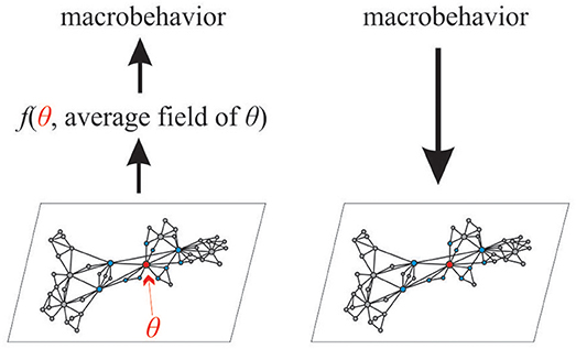
Figure 1. Typical description of the dynamics arising from the interaction of numerous basic elements over a complex network that focuses on the global behavior of the system (left). Such an approach, however, comes with a price of not being able to quantify dynamics of individual elements within the system. In this paper, we address this problem by adopting statistical properties of the macroscopic dynamics in order to infer the behavior of individual units.

In this paper, we address this issue by posing the inverse question. Rather than inferring the global dynamics by combining the behavior of single elements within the dynamical system, we ask whether it is possible to construct a description of the dynamics of the individual elements, provided information about the network's global behavior. We approach the problem by considering statistical properties of the global variable.

Frequently, the macrovariables observed in complex networks display emergent properties of spatial and/or temporal scale-invariance. These are manifested by, for example, the inverse power scaling of waiting-time probability density functions (PDFs) between events, such as communication instances in human interactions or occurrence of earthquakes. At the same time, the inverse power laws (IPLs) that characterize the emergent macroscopic behavior are reminiscent of particle dynamics near a critical point, where a dynamic system undergoes a phase transition [19]. However, despite the advances made by the renormalization group approach and self-organized criticality theories that have shown how scale-free phenomena emerge at critical points, the issue of determining how the emergent properties influence the microdynamics of individual units of the system remains open.

Herein, we address the problem of quantifying the response of an individual unit to the dynamics of the collective. This is done by taking advantage of the fractional calculus apparatus, whose utility arises from its ability to seamlessly incorporate the IPL statistics into its dynamics. The phase transitions that characterize many complex systems suggest the wisdom of using a generic model from the Ising universality class to characterize system dynamics. It is then possible to demonstrate that the individual trajectory response to the collective dynamics of the system is described by a linear fractional differential equation. This is achieved through a subordination procedure without the necessity of linearizing the underlying dynamics. Following this procedure, it is shown that the analytic solution to the linear fractal differential equation retains the influence of the nonlinear network dynamics on the behavior of the individual. Moreover, the solution to the fractional equation of motion suggests a new direction for designing mechanisms to control the dynamics of complex networks.

In section 2, we sketch out the mathematics of the dynamical decision making model (DMM), introduce renewal events, and subordinate the behavior of the individual to the mean field behavior of the network. In section 2.2, the dynamics of the individual is determined from the subordination theory to be a tempered fractional differential equation. The exact solution to this equation is given by an attenuated Mittag-Leffler function, which is fitted to the numerical solution of the DMM equation. In section 4, we discuss some implications of the high quality convergence of the analytical and numerical results of this complex network.

2. Complex Network Dynamics

As demonstrated by Grinstein et al. [20], any discrete system, defined by means of local interactions, with symmetric transitions between states and randomness that originate from the presence of a thermal bath or internal causes belongs to the universality class of kinetic Ising models. One such system is the DMM [21–23] and is the one we implement herein. Each individual unit s_i of the model is a stochastic oscillator and can be found in either of the two states, +1 or −1. The dynamics are defined in terms of the probability of an individual to be in either state, and it is modeled by the coupled two-state master equation,

$\begin{array}{ll}\frac{d\text{p}(t)}{dt}=g_0\left[\text{I}-21\right]\text{p}(t),& (1)\end{array}$

where I and 1 are the 2 × 2 identity and unit matrices, respectively. The probability of being in one of the two states (+1, −1), $\text{p}(t)={\left[p_1(t),p_2(t)\right]}^{⊺}$, defines a Markovian telegraph noise, with symmetric and constant rate of changing states 0 < g₀ < 1.

Positioning N such individuals at the nodes of a complex network introduces coupling between them [21, 22], which, here, is limited to the nearest neighbor interactions. The influence that unit s_i experiences due to the presence of its neighbors is expressed by a modification of its transition rate

$\begin{array}{lll}{g}_{12}^{(i)}(t)& =& g_{0}exp\left[-\frac{K}{M^{(i)}}\left(M_1^{(i)}(t)-M_2^{(i)}(t)\right)\right],\\ g_{21}^{(i)}(t)& =& g_{0}exp\left[\frac{K}{M^{(i)}}\left(M_1^{(i)}(t)-M_2^{(i)}(t)\right)\right],& (2)\end{array}$

which becomes a time dependent variable. Here, K is the strength of the coupling between nodes, 0 < K < ∞, constant for all nodes in the network. The variable M⁽ⁱ⁾ denotes the degree of the node i, and $M_{1,2}^{(i)}(t)$ denotes, respectively, the count of the nearest neighbors in states s_i(K, t) = 1 and s_i(K, t) = −1 at time t. As single units s_i change their states, quantities $M_1^{(i)}(t)$ and $M_2^{(i)}(t)$ fluctuate in time, while their sum is always conserved $M_1^{(i)}(t)+M_2^{(i)}(t)=M^{(i)}$. In this paper, we consider the case of a regular two-dimensional lattice, where M⁽ⁱ⁾ = 4 and $0\le M_{1,2}^{(i)}(t)$ for all the nodes. The single unit in isolation corresponds to the case of K = 0. When the coupling constant K > 0, a unit in state +1(−1) makes a transition to the state −1(+1) faster or slower according to whether $M_2^{(i)}(t)>M_1^{(i)}(t)$ or $M_1^{(i)}(t)>M_2^{(i)}(t)$, respectively.

Time-dependent transition rates modify the two-state master (Equation 1) to take the form

$\begin{array}{ll}\frac{d{\text{p}}^{(i)}(t)}{dt}={\text{G}}_i(t){\text{p}}^{(i)}(t),& (3)\end{array}$

where the matrix of rates G_i(t) is defined as

$\begin{array}{ll}{\text{G}}_i(t)=\left(\begin{array}{cc}-g_{12}^{(i)}(t)& g_{21}^{(i)}(t)\\ -g_{21}^{(i)}(t)& g_{12}^{(i)}(t)\end{array}\right),& (4)\end{array}$

and p⁽ⁱ⁾(t) is the probability of the element i = 1, 2, …, N in the network at time t and is normalized such that $p_1^{(i)}(t)+p_2^{(i)}(t)=1$ for every i.

Dynamics of an entire network is described by a system of N such coupled equations, resulting in a highly nonlinear system [23], containing 6N dynamic variables $\left(p_1^{(i)}(t),p_2^{(i)}(t),g_{12}^{(i)}(t),g_{21}^{(i)}(t),M_1^{(i)}(t),M_2^{(i)}(t)\right)$. This number of coupled variables prevents the successful application of analytic methods, as these are usually adopted to solve problems that involve only a few coupled time-dependent differential equations. Instead, extensive numerical calculations are supplemented by an analytic formulation of the evolution of a global variable.

As depicted in Figure 2B, the global behavior of the model, defined by the fluctuations of the mean field variable

$\begin{array}{ll}\xi (K,t)=\frac{1}{N}{\displaystyle \underset{i=1}{\sum ^N}}{s}_i(K,t),& (5)\end{array}$

shows a pronounced transition as a function of the control parameter K. While in Figure 2A, the single elements appear to be essentially unchanged by their interactions with the rest of the network, the global variable shifts from a configuration dominated by randomness to one in which strong interactions give rise to long-lasting majority states shown in Figure 2B. Note that the origin of the random fluctuation in the DMM is the finite size of the network, which has nothing to do with the thermal fluctuations in the Ising model of magnetization.

FIGURE 2

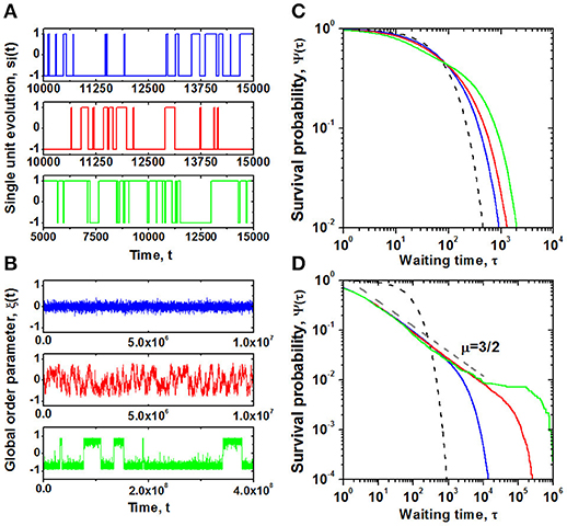
Figure 2. Behavior of a discrete, two-state dynamic unit on a two-dimensional lattice. Temporal evolution and corresponding survival probability Ψ(τ) for the transitions between two states for the single unit s_i(t) of the system, presented on panels (A,C), respectively, are compared with the behavior and statistical properties of the global order parameter ξ(t), showed on panels (B,D). Simulations were performed on a lattice of size N = 50 × 50 nodes, with periodic boundary conditions, for g₀ = 0.01 and increasing values of the control parameter K. Blue, red, and green lines correspond to K = 1.50, 1.70, and 1.90, respectively. The critical value of the control parameter is K_C ≈ 1.72. Black dashed line on the plots of Ψ(τ) denotes an exponential distribution, with the decay rate g₀.

To characterize the changes in the temporal properties of the micro- and macro-variables, we evaluate the survival probability function, Ψ(τ), of time intervals τ between consecutive events defined as changes of the state or crossing of the zero-axis, for the single element or the global variable, respectively. These calculations unveil modest deviations of Ψ(τ) for a single individual from the exponential form, Ψ(τ) = exp(−g₀τ), that characterizes single non-interacting elements, as shown in Figure 2C. Clearly, the influence of the network on the behavior of the individual does not appear to induce a significant change in the latter. Despite such a modest change in the behavior of the individual, the global variable manifests IPL statistics, as depicted in Figure 2D. Thus, the following question arises: To what extent are individual opinions within a complex network influenced by the network dynamics?

2.1. Renewal Events

Many physical processes, for example earthquakes, radioactive decay, and social processes, such as making a decision, can be viewed as particular events. A characteristic property of an event is that it's onset can be precisely localized in time, even if its occurrence has extended consequences in space. Thus, the dynamics of a process characterized by events is described in terms of the probability of an event occurring, rather than by a more traditional Hamiltonian approach.

The process of event occurrence is characterized by the waiting-time PDF ψ(τ), which specifies the distribution of times between consecutive events. The probability for an event to occur in the short time interval [t, t + dt] is given by

$\begin{array}{ll}\psi (t)dt=Pr(t<\tau <t+dt),& (6)\end{array}$

where τ is measured from the occurrence of the previous event. Consequently, one can define the survival probability Ψ(τ) as the probability that no event occurs up to the time since the last event as

$\begin{array}{ll}\text{Ψ}(\tau )\equiv {\displaystyle \underset{\tau }{\stackrel{\infty }{\int }}}\psi (t)dt.& (7)\end{array}$

As a consequence of this integral, the waiting-time PDF can be written as

$\begin{array}{ll}\psi (t)=-\frac{d\text{Ψ}(t)}{dt},& (8)\end{array}$

and the PDF ψ(τ) is a properly normalized function,

$\begin{array}{l}{\displaystyle \underset{0}{\stackrel{\infty }{\int }}}\psi (\tau )d\tau =1,\end{array}$

since it is assumed that an event occurs somewhere within the time interval (0, ∞). It is also true that no event occurs at time t = 0, which means that the survival probability Ψ(0) = 1.

A particular class of events can be defined, renewal events, that reset the clock of the system to an initial state instantaneously after their occurrence. After a renewal event takes place, the system evolves in time independently of whatever occurred earlier, having no memory of previous instances in which such an event occurred. Some examples of renewal events found in physics include anomalous diffusion of tagged particles inside living cells, blinking quantum dots, and defects arising in the weak turbulence regime of liquid crystals.

The renewal character of events is captured by the probability of n events occurring as follows. First, one assumes that an event occurs at time t = 0, thus, ψ₀(t) = δ(t). Next, the first event occurs at time t > 0, taking place with the probability ψ₁(t) = ψ(t). Subsequently, the probability for event n in a sequence to occur at time t is expressed in terms of probabilities of earlier events by the correlation chain condition

$\begin{array}{ll}{\psi }_n(t)=\stackrel{t}{{\displaystyle \underset{0}{\int }}}{\psi }_{n-1}(t^{\prime }){\psi }_1(t-t^{\prime })d{t}^{\prime }.& (9)\end{array}$

Frequently, experimentally observed waiting-time PDFs are exponential, but quite often in complex networks they are IPLs. For the purpose of this paper, we define the waiting-time PDF in terms of the hyperbolic distribution

$\begin{array}{ll}\psi (t)=\frac{(\mu -1)T^{\mu -1}}{{(T+t)}^{\mu }}.& (10)\end{array}$

If the events are generated by an ergodic process, then μ > 2, and the first moment of the hyperbolic PDF is

$\begin{array}{ll}\langle t\rangle =\stackrel{\infty }{{\displaystyle \underset{0}{\int }}}t\psi (t)dt=\frac{T}{\mu -2}.& (11)\end{array}$

In the framework of renewal theory, Equation (11) denotes the average time that one would have to wait between successive events. However, when μ < 2, the process is non-ergodic, and the mean value of the distribution diverges. In the non-ergodic case, T becomes a characteristic time scale of the process.

2.2. Subordination of Time

The notion of different clocks associated with different physical systems arises naturally in physics; the linear Lorentz transformation in relativistic physics being probably the most familiar example. Thanks to the recent availability of time-resolved data, biological, and social sciences have also started adopting the notion of multiple clocks, distinguishing between cell-specific and organ-specific clocks in biology and person-specific and group-specific clocks in sociology. Of course, the notion of subjective and objective time dates back to the middle of the nineteenth century with the introduction of the empirical Weber-Fechner law [24].

However, the striking difference between the clocks of classical physics and natural sciences is that the relations between the latter clocks are nonlinear. While the global activity of an organ, such as the brain or the heart, might be characterized by quite regular, often periodic fluctuations, the activity of single neurons demonstrates burstiness and noisiness. Similarly, in a society, people operate according to their individual schedules, not always being able to perform particular actions in the same global time frame. Thus, owing to the stochastic behavior of one or both clocks, a probabilistic transformation between times is necessary. An example of such a transformation is the subordination procedure.

We begin by defining two clocks. The first clock records a discrete operational time n, which measures the time T(n) of an individual. The second clock records the continuous chronological time t, which measures the time T(t) that a system of individuals have agreed upon. If each advancement of the discrete clock n is thought of as an event, then the relation between the operational time and chronological time can be given by the waiting-time PDF of those events in chronological time ψ(t). Assuming a renewal property for events, as given by chain condition from renewal theory (Equation 9), one can relate operational time to chronological time by

$\begin{array}{ll}\langle T(t)\rangle ={\displaystyle \underset{n=1}{\sum ^{\infty }}}\stackrel{t}{{\displaystyle \underset{0}{\int }}}\text{Ψ}(t-t^{\prime }){\psi }_n(t^{\prime })T(n)d{t}^{\prime }.& (12)\end{array}$

Every advancement of the operational clock is an event, which in the chronological time occurs at time intervals drawn from the renewal waiting-time PDF. Because of this randomness, one needs to sum over all events, and the result is an average over many realizations of the transformation.

As an example, consider the behavior of a two-state operational clock, whose evolution is shown in Figure 3. In operational time, the clock switches back and forth between its two states at equal unit time intervals. In chronological time, however, this regular behavior is significantly distorted. In the figure, the time transformation was taken to be an IPL PDF of waiting times. Thus, a single time step in the operational time corresponds to a time interval being a random number drawn from ψ(t) in chronological time. The long tail of the IPL PDF leads to especially strong distortions of the operational time trajectory, since there exist a non-zero probability of drawing very large time intervals between events. However, since the transformation between the operational and chronological time scales involves a random process, one needs to consider infinitely many trajectories in the chronological time, which leads to the average behavior of the clock in the chronological time denoted in Equation (12) by the bracket.

FIGURE 3

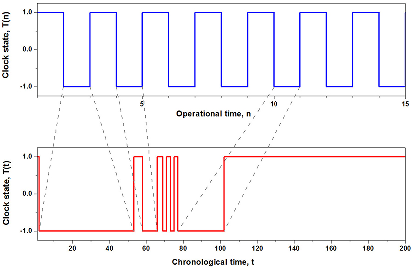
Figure 3. The upper curve is the regular transition between the two states of the individual in operational time. The lower curve is the subordination of the transition times to an IPL PDF to obtain chronological time.

We note that the time subordination procedure can also be used to model communication delays in the system. However, contrary to frequently used approaches, where individual units of the system are subordinated to model the interaction delay, here, we adopt the statistics of the macroscopic variable to derive the behavior of the interacting individual units. The coupling between units causes them to deviate from the Poisson behavior of an individual non-interacting unit. However, as illustrated in Figure 2, the time scale of interacting units is orders of magnitude that are smaller than the time scale of the macroscopic variable. Thus, we use the statistical properties of the macroscopic variable to provide a first-order estimate of the single unit dynamics. As such, we adopt a top-down approach, which is different from the bottom-up approach adopted for the consideration of communication delays.

3. Complex Network Subordination

To determine the network's influence on the dynamics of the individual, we adapt the subordination argument of the preceding section and relate the time scale of the macro-variable ξ(K, t) to the time scale of the micro-variable s_i(K, t). The two-state master equation for a single isolated individual in discrete time n in steps of Δτ is

$\begin{array}{ll}\phi (n+1)-\phi (n)=-g_0\Delta \tau \phi (n),& (13)\end{array}$

where the notations φ(n) = φ(nΔτ) and φ = p₁ − p₂ depict the difference in probabilities for the typical individual to assume one of the two states. The solution to this discrete equation is

$\begin{array}{ll}\phi (n)={(1-g_0\Delta \tau )}^n\phi (0),& (14)\end{array}$

which, in the limit g₀ Δ τ < < 1, becomes an exponential. However, when the individual is a part of a network, the dynamics are not so simple.

Adopting the subordination interpretation, we define the discrete index n as an individual's operational time that is stochastically connected to the chronological time t, in which the global behavior is observed. We assume that the chronological time lies in the interval (n − 1) Δτ ≤ t ≤ n Δτand, consequently, the equation for the average dynamics of the individual probability difference is given by [25]

$\begin{array}{ll}\langle \phi (t)\rangle ={\displaystyle \underset{n=1}{\sum ^{\infty }}}\stackrel{t}{{\displaystyle \underset{0}{\int }}}\text{Ψ}(t-t^{\prime }){\psi }_n(t^{\prime })\phi (n)d{t}^{\prime }.& (15)\end{array}$

Here, the time t in the waiting-time PDF ψ(t) is determined from the derivative of the survival probability. The empirically determined analytic expression for the survival probability is

$\begin{array}{ll}\text{Ψ}(t)={\left(\frac{T}{T+t}\right)}^{\mu -1}{e}^{-ϵt}.& (16)\end{array}$

The dominant behavior of the empirical survival probability is an IPL as indicated in Figure 2D. However, at early times, the probability of not making a transition approaches the constant value of one; at late times, the probability of not making a transition at a given time decays exponentially; it is in the middle range, where the probability is an IPL. The extent of the IPL range of the survival probability is determined by the empirical values of T, μ, and ϵ, and from Figure 2D, the value of ϵ is seen to become smaller as the control parameter K increases. The IPL functional form of the PDF results from the behavior of the survival probability Ψ(τ) of the global variable depicted in Figure 2D, with μ = 3/2.

Using a renewal theory argument, Pramulkkul et al. [25] show that Equation (15) expressed in terms of Laplace transform variables indicated by $\hat{f}(u)$ for the time-dependent function f(t) has the form

$\begin{array}{ll}\langle \hat{\phi }(s)\rangle =\frac{\phi (0)}{u+ϵ+{\lambda }_0\hat{\Phi }(u+ϵ)}& (17)\end{array}$

where λ₀ ≡ g₀ Δ τ and $\hat{\Phi }(u+ϵ)$ is the Laplace transform of the Montroll-Weiss memory kernel [25, 26],

$\begin{array}{ll}\hat{\Phi }(u+ϵ)=\frac{(u+ϵ)\hat{\psi }(u+ϵ)}{1-\hat{\psi }(u+ϵ)}.& (18)\end{array}$

Note that u is replaced by u + ϵ in the Laplace transforms, because the exponential truncation of the empirical survival probability shifts the index on the Laplace transform operation. The asymptotic behavior of an individual in time is determined by considering the waiting-time PDF as u → 0,

$\begin{array}{ll}\hat{\psi }(u+ϵ)\approx 1-\Gamma (1-\alpha )T^{\alpha }{(u+ϵ)}^{\alpha }\mathrm{\text{;}}0<\alpha =\mu -1<1,& (19)\end{array}$

so that Equation (17) reduces to

$\begin{array}{ll}\langle \hat{\phi }(u)\rangle =\frac{\phi (0)}{u+ϵ+{\lambda }^{\alpha }{(u+ϵ)}^{1-\alpha }}.& (20)\end{array}$

The inverse Laplace transform of Equation (20) yields the tempered rate equation

$\begin{array}{ll}{({\partial }_t+ϵ)}^{\alpha }\langle \phi (t)\rangle =-{\lambda }^{\alpha }\langle \phi (t)\rangle ,& (21)\end{array}$

where the operator ${\partial }_t^{\mu -1}\left[·\right]$ is the Caputo fractional derivative for 0 < α = μ − 1 < 1 [11] and

$\begin{array}{ll}\lambda T={\left[g_0\Delta \tau /\Gamma (2-\mu )\right]}^{\frac{1}{\mu -1}}.& (22)\end{array}$

Note that owing to the dichotomous nature of the states, 〈φ(t)〉 is the average opinion of the individual s_i(K, t).

The solution of the asymptotic fractional master equation (Equation 21) for a randomly chosen unit within the network is given by an exponentially attenuated Mittag-Leffler function (MLF):

$\begin{array}{ll}\langle \phi \left(t\right))\rangle =\phi \left(0\right))E_{\alpha }\left(-{\left(\text{λ}t\right)}^{\alpha }\right)\exp \left[-\in t\right]& (23)\end{array}$

and the MLF is defined by the series

$\begin{array}{ll}{E}_{\alpha }\left(z\right)\equiv {\displaystyle \sum _{n=0}^{\infty }\frac{z^n}{\Gamma \left(n\alpha +1\right)}}.& (24)\end{array}$

The MLF is a stretched exponential at early times and an IPL at late times, with α = μ − 1 being the IPL index in both domains.

3.1. Comparisons With Numerics

We test the above analysis with numerical simulations of the dynamic network on a two-dimensional lattice with nearest-neighbor interactions in all three regions of DMM dynamics: subcritical, critical, and supercritical. The time-dependent average opinion of a randomly chosen individual is presented in Figure 4, where the average is taken over 10⁴ independent realizations of the dynamics in the subcritical, critical, and supercritical regimes.

FIGURE 4

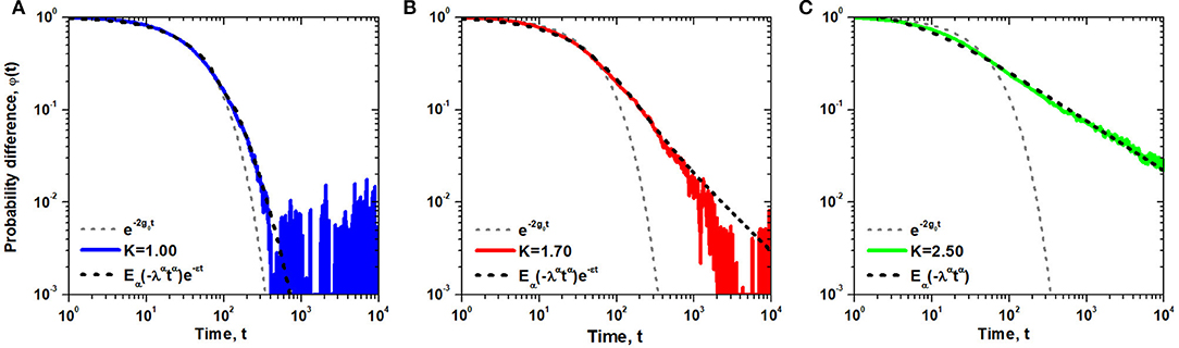
Figure 4. The probability difference 〈φ(t)〉 estimated as an average over an ensemble of 10⁴ independent realizations of single element trajectories. Each trajectory corresponds to evolution of a randomly selected node within a N = 100 × 100 lattice network, with g₀ = 0.01 and the same initial condition s_i(0) = 1. The parameter values for the numerical data are given in Figure 2 and from left to right K = 1.0 (A), 1.7 (B), 2.5 (C), respectively. The fit of the exponentially truncated MLF to the numerical calculations is summarized in Table 1.

A comparison with the exponential form of 〈φ(t)〉 for an isolated individual indicates that the influence of the network on the individual's dynamics clearly persists for increasingly longer times with increasing values of the control parameter within the network. The parameters μ and λ of Equation (23) obtained through fitting numerical results of Figure 4 with the MLF are summarized in Table 1. It is evident that the influence of the network dynamics on the individual is greatest at long times. The deviation of the analytic solution from the numerical calculation is evident for values of the control parameter at and below the critical value. The analytical prediction is least reliable at extremely long times in the subcritical domain. Consequently, the response of the individual to the group mimics the group's behavior most closely when the control parameter is equal to or greater than the critical value.

TABLE 1

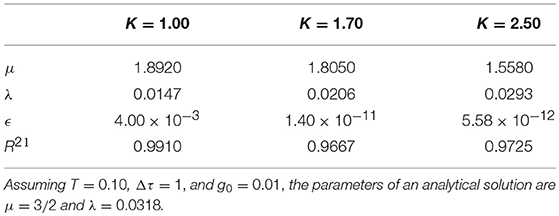
Table 1. The probability difference 〈φ(t)〉 of Figure 4 is fitted with the MLF using an algorithm developed by Podlubny [27].

4. Discussion

Herein, the subordination procedure provides an equivalent description of the average dynamics of a single individual within a complex network, in terms of a linear fractional differential equation. The fractional rate equation is solved exactly, determining the Poisson statistics of the isolated individual becomes attenuated Mittag-Leffler statistics, owing to the interaction of that individual with the other members of a complex dynamic network.

Consequently, an individual's simple random behavior, when isolated, is replaced with behavior that might serve a more adaptive role in social networks. We conjecture that the behavior of the individual is generic, given that the DMM network dynamics belong to the Ising universality class. Members of this universality class share the critical temporal behavior [28] that drives the subordination process. It is the renewal property of the event statistics, which, through the subordination process, gives rise to the linear fractional master equation for the typical individual's dynamics. The solution to the tempered fractional rate equation manifests the subsequent robust behavior of the individual; it remains to be determined just how robust the behavior of the individual is relative to control signals that might be driving the network.

As pointed out by Liu et al. [29], the ultimate understanding of complex networks is reflected in the ability to control them. Recent observations of the interconnectedness of infrastructure networks [30], facilitating the spread of failures [31] or the tight coupling between banking institutions, posing a danger to the stability of global financial system [32], demonstrate the importance of developing a systematic approach to influence and/or control the complex networks. The analysis presented here provides an alternative attempt to address this need directly. Subordination suggests a way to impose the conditions of traditional control theory [33] onto the complex network dynamics by, first, expressing the underlying nonlinear network dynamics in the form of a linear fractional equation of motion. This approach at addressing control will be pursued in a future publication.

Author Contributions

BW developed the theoretical formalism and performed the analytic calculations. MT performed numerical simulations. Both authors discussed the results and contributed to the final manuscript.

Conflict of Interest Statement

The authors declare that the research was conducted in the absence of any commercial or financial relationships that could be construed as a potential conflict of interest.

Acknowledgments

The authors acknowledge the US Army Research Laboratory for supporting this research.

Footnotes

1. ^ Adjusted goodness of fit, $R^2=1-\frac{S{S}_{reg}/(n-\kappa )}{S{S}_{tot}/(n-1)}$, is defined as the ratio of the sum of squared residues for the nonlinear fit with the MLF (SS_reg) and for the fit to the average value of data points (SS_tot), where n is the number of data points and κ is the number of free parameters being estimated.

References

1. Newman MEJ. Networks, An Introduction. New York, NY: Oxford University Press (2018).

2. Barabasi AL. Network Science. Cambridge, UK: Cambridge University Press (2016).

Google Scholar

3. Bianconi G. Multilayer Networks: Structure and Function. Oxford, UK: Oxford University Press (2018).

Google Scholar

4. Podlubny I. Frational Differential Equations. Sand Diego, CA: Academic Press (1999).

5. West BJ, Bologna M, Grigolini P. Physics of Fractal Operators. New York, NY: Springer (2003).

Google Scholar

6. Magin RL. Fractional Calculus in Bioengineering. Danbury, CT: Begell House (2006).

Google Scholar

7. Pastor-Satorras R, Castellano Claudio, Van Mieghem P, Vespignani A. Epidemic processes in complex networks. Rev Mod Phys. (2015) 87:925–79. doi: 10.1103/RevModPhys.87.925

CrossRef Full Text | Google Scholar

8. Hernandez-Urbina V, Herrmann JM, Spagnolo B. Neuronal avalanches in complex networks. Cogent Phys. (2016) 3:1150408. doi: 10.1080/23311940.2016.1150408

CrossRef Full Text | Google Scholar

9. Castellano C, Fortunato S, Loreto V. Statistical physics of social dynamics. Rev Mod Phys. (2009) 81:591–646. doi: 10.1103/RevModPhys.81.591

CrossRef Full Text | Google Scholar

10. Herrmann R. Fractional Calculus: An Introduction for Physicists. New York, NY: World Scientific (2011).

11. West BJ. Fractional Calculus View of Complexity: Tomorrow's Science. Boca Raton, FL: CRC Press (2016).

Google Scholar

12. Magin RL. Models of diffusion signal decay in magnetic resonance imaging: capturing complexity. Concepts Magn Reson Part A (2018) 45A:e21401. doi: 10.1002/cmr.a.21401

CrossRef Full Text | Google Scholar

13. Meerschaert MM, West BJ, Zhou Y. Future directions in fractional calculus research and applications. Chaos Solit Fract. (2017) 102:1. doi: 10.1016/j.chaos.2017.07.011

CrossRef Full Text | Google Scholar

14. Flack A, Nagy M, Fiedler W, Couzin ID, Wikelski M. From local collective behavior to global migratory patterns in white storks. Science (2018) 360:911–4. doi: 10.1126/science.aap778

PubMed Abstract | CrossRef Full Text | Google Scholar

15. Bette HM, Habel L, Emig T, Schreckenberg M. Mechanisms of jamming in the Nagel-Schreckenberg model for traffic flow. Phys Rev E (2017) 95:012311. doi: 10.1103/PhysRevE.95.012311

PubMed Abstract | CrossRef Full Text | Google Scholar

16. Yang Y, Nishikawa T, Motter AE. Small vulnerable sets determine large network cascades in power grids. Science (2017) 358:eaan3184. doi: 10.1126/science.aan3184

PubMed Abstract | CrossRef Full Text | Google Scholar

17. Dorogovtsev SN, Goltsev AV, Mendes JFF. Critical phenomena in complex networks. Rev Mod Phys. (2008) 80:1275–335. doi: 10.1103/RevModPhys.80.1275

CrossRef Full Text | Google Scholar

18. Toda M, Kubo R, Saito N. Statistical Physics I: Equilibrium Statistical Mechanics. Berlin: Springer (2004).

19. Christensen K, Moloney NR. Complexity and Criticality. London, UK: Imperial College Press (2005).

Google Scholar

20. Grinstein G, Jayaprakash C, Yu H. Statistical mechanics of probabilistic cellular automata. Phys Rev Lett. (1985) 55:2527–30.

PubMed Abstract | Google Scholar

21. Bianco S, Geneston E, Grigolini P, Ignaccolo M. Renewal aging as emerging property of phase synchronization. Phys A (2008) 387:1387. doi: 10.1016/j.physa.2007.10.045

CrossRef Full Text | Google Scholar

22. Turalska M, Lukovic M, West BJ, Grigolini P. Complexity and synchronization. Phys Rev E (2009) 80:021110. doi: 10.1103/PhysRevE.80.021110

PubMed Abstract | CrossRef Full Text | Google Scholar

23. Turalska M, West BJ, Grigolini P. Temporal complexity of the order parameter at the phase transition. Phys Rev E (2011) 83:061142. doi: 10.1103/PhysRevE.83.061142

PubMed Abstract | CrossRef Full Text | Google Scholar

24. Fechner GT. Elemente der Psychophysik. Leipzig: Breitkopf and Härtel (1860).

Google Scholar

25. Pramukkul P, Svenkeson A, Grigolini P, Bologna M, West BJ. Complexity and the fractional calculus. Adv Math Phys. (2013) 2013:1–7. doi: 10.1155/2013/498789

CrossRef Full Text | Google Scholar

26. Montroll WE, Weiss G. Random walks on lattices. J Math Phys. (1965) 6:167–81.

Google Scholar

27. Gorenflo R, Loutchko J, Luchko Y. Computation of the Mittag-Leffler function E_{α, β}, (z) and its derivative. Fract Calc Appl Anal. (2002) 5:491–518.

Google Scholar

28. Turalska M, West BJ, Grigolini P. Role of committed minorities in times of crisis. Sci Rep. (2013) 3:1371. doi: 10.1038/srep01371

PubMed Abstract | CrossRef Full Text | Google Scholar

29. Liu Y, Slotine J, Barabási A. Controllability of complex networks. Nature (2011) 473:167–73. doi: 10.1038/nature10011

PubMed Abstract | CrossRef Full Text | Google Scholar

30. Brummitt CD, D'Souza RM, Leicht EA. Suppressing cascades of load in interdependent networks. Proc Natl Acad Sci USA. (2012) 109:680–9. doi: 10.1073/pnas.1110586109

PubMed Abstract | CrossRef Full Text | Google Scholar

31. Buldyrev SV, Parshani R, Paul G, Stanley HE, Havlin S. Catastrophic cascade of failures in interdependent networks. Nature (2010) 464:1025–8. doi: 10.1038/nature08932

PubMed Abstract | CrossRef Full Text | Google Scholar

32. Battiston S, Puliga M, Kaushik R, Tasca P, Caldarelli G. DebtRank: too central to fail? Financial networks, the FED and systemic risk. Sci Rep. (2012) 2:541. doi: 10.1038/srep00541

PubMed Abstract | CrossRef Full Text | Google Scholar

33. Brockett R. Stochastic Control. Lecture Notes. Cambridge, MA: Harvard University (2009).

Google Scholar