 Masahiko Higashi
 Reiji Suzuki
 Takaya Arita
95% of researchers rate our articles as excellent or good
Learn more about the work of our research integrity team to safeguard the quality of each article we publish.
Find out more
ORIGINAL RESEARCH article
Front. Phys. , 28 August 2018
Sec. Interdisciplinary Physics
Volume 6 - 2018 | https://doi.org/10.3389/fphy.2018.00088
This article is part of the Research Topic Coordination and Cooperation in Complex Adaptive Systems: Theory and Application View all 14 articles
The role and importance of social learning have been investigated by many researchers because it is observed in many animals and is expected to play a significant role in cultural phenomena. We explore the coevolution between individual learning and social learning on a rugged fitness landscape as a realistic condition in which they can interact with each other. We demonstrate that social learning allows individuals not to have adaptive traits innately, and thus, has two important roles to enhance individual fitness. First, social learning spreads and keeps the adaptive phenotypes acquired by individual learning. Second, social learning enables individuals to explore a wide range of fitness landscape by the increased population diversity. Based on the difference of the roles of individual and social learning, they can work complementarily in the course of adaptive evolution on the rugged fitness landscape.
Animals adapt to their environment by two different mechanisms working on two levels, evolution and learning. Evolution is a population level mechanism and learning is an individual level mechanism. There have been a lot of discussion on the effects of learning on the course of evolution. Baldwin, a pioneer in epigenetic evolutionary theory, proposed a possible scenario which is now called Baldwin effect that explains how evolution and learning interact with each other [1]. It consists of the following two steps [2]. (1) Some agents acquire adaptive phenotypes by learning, and then, they increase in population. (2) Because of the learning cost, agents which have the adaptive phenotypes innately become more adaptive than other agents, so the population evolves to have adaptive phenotypes innately i.e., a genetic assimilation of adaptive phenotypes. Through these two steps, learning facilitates the evolution.
Hinton and Nowlan devised a simple computational model that shows learning can accelerate evolution, and they associated this phenomenon with the Baldwin effect [3]. However, individuals in the model only used individual learning based on trial-and-error. Learning can be classified into individual learning (e.g., trial-and-error process) and social learning (e.g., imitation process). Via individual learning animals adapt to their environment by using only their own experience while via social learning they adapt to their environment by using other animals' experience. In general, it is considered that social learning affect evolution of animals significantly, because it allows animals to acquire adaptive behavior without paying the cost of trial-and-error process, and also, the adaptive behavior can be evolved cumulatively through generations by the imitation between adults and offspring. These types of transmission are necessary to create culture, and from the interest of cultural evolution, social learning has been investigated for a long time from many points of view.
The two major focuses of the research on social learning having been the conditions under which social learning evolves and the way of social learning. In the research focusing on the conditions, researchers mainly investigated the effects of fluctuation and structure of environment, and successfully showed that social learning is favored in stable and simple environment. For example, on the effect of fluctuation on environment, Rendell et al. [4] and Jones et al. [5] found that when the environment is varied or intense, social learning is disfavored. On the effect of structure of environment, Tamura et al. [6] developed a mathematical model to explore the effect of social networks on social learning and revealed that social networks disfavor the social learning. Kobayashi et al. [7] also developed an island migration model and revealed that spatial structures disfavor the social learning. The way of social learning can be approached from at least two aspects: “when” and “whom” they learn from Laland [8]. As a study focusing on “when,” Enquist et al. [9] found that “critical social learning” that does social learning during having no information about the environment and then does individual learning, is superior to pure social learning. Rendell et al. [4] also revealed that the “conditional social learning” that does social learning only when individual learning fails, is superior to pure social learning. As a study focusing on “whom,” Mesoudi [10] found that “copy-successful-individuals” strategy is more adaptive than individual learning by experimental simulation using human subjects. “whom” aspect is linked to the biases in information transmission. Specifically, it has been shown that the conformist bias is adaptive under a broad range of environmental conditions [11–14].
However, most of computational or mathematical research assumed the transfer of very simple information (typically, which of two behaviors is correct) that sometimes becomes absolute [6, 7, 9, 11–14]. This situation could be interpreted as the evolution on a fitness landscape with a single peak of which location might change occasionally. However, in the real world, the fitness landscape should have many peaks as local optima in general. Therefore, we explore the interactions between individual learning and social learning on a rugged fitness landscape as a more realistic condition. The purpose of our study is to clarify evolutionary roles of individual and social learning on a rugged fitness landscape in the context of the Baldwin effect. We adopted a minimal fitness function [15] that represents a multi-modal fitness landscape in which there is a trade-off between the adaptivity of individuals and the strength of nonlinear epistatic interactions among multiple phenotypes. We constructed an agent-based evolutionary model in which each individual can accommodate its plastic phenotypes using both individual learning based on trial-and-error and social learning based on imitation of multiple phenotypes from the most adaptive individual.
There are N individuals in a population and each individual has M traits ti (i = 0 … M-1) as shown in Table 1. Each gene gi (i = 0… M-1) in a M-length chromosome GI represents the initial value of the corresponding trait ti, taking an integer value within the range [1, M]. Each individual has another M-length chromosome GP (pi (i = 0… M − 1)) which decides whether the corresponding trait is plastic (“1”) or not (“0”). Each row of plastic traits is highlighted in Table 1. Plastic traits can be changed through the individual or social learning process (described later). Each individual also has a gene s which represents the probability of performing social learning instead of individual learning. s has a real value in the range of [0, 1]. The trait values ti are determined in the range of gi±1 by learning. So as to evaluate the fitness of each set of traits, we adopted the following fitness function [15]:
where num(n) represents the number of traits of which phenotypic value is n. The fitness is determined by a group of traits which have the same values using Equations (1, 2). Equation (2) shows that the trait group of n yields the fitness value n if its group size (num(n)) is greater than or equals to n, and Equation (1) shows that the highest f (n) of the trait group defined by Equation (2) is adopted as the fitness of the trait set. For example, the fitness of the trait set in Table 1 is 6 because the number of 6 in the traits is 6 and at the same time, it is the highest number among those which satisfy the condition in Equation (2), as illustrated in Table 2.
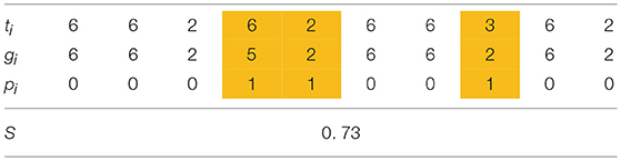
Table 1. An example of an individual (M = 10).
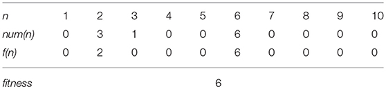
Table 2. Fitness evaluation of the trait set in Table 1.
This fitness function has the following two characteristics, and thus the fitness landscape is rugged as illustrated in Figure 1.
1) The higher the fitness of trait group is, the harder to get it, because the minimum size necessary for the trait group to express its adaptivity becomes larger.
2) When n ≥ M/2 it is impossible to satisfy both conditions num(n) ≥ n and num(n + 1) ≥ n + 1.
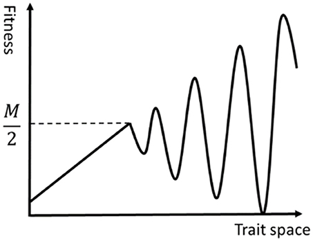
Figure 1. An image of a rugged fitness landscape defined by Equations (1, 2).
The benefit for using this fitness landscape is that we can explicitly grasp the contribution of each phenotypic value on the fitness and the progress of the evolution while keeping the ruggedness of the landscape high.
We assume an intergenerationally overlapped population that consists of N/2 parents and N/2 offspring. Figure 2 illustrates the population structure composed of two types of (i.e., parent and offspring) individuals. In each generation, all individuals simultaneously learn individually or socially L times regardless of being parents or offspring. In other words, the individuals learn L times with their parents and themselves after they are born in a generation, and then they become parents and learn L times with their offspring and themselves in the next generation. In each learning step, each individual chooses social learning with its genetically determined probability s, meaning it chooses individual learning with the probability 1-s. The way of learning is defined as follows.
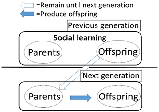
Figure 2. The overlap between generations in the model.
The individual who chose social learning selects and imitates another individual who got the highest fitness in the last learning step. It makes each plastic trait closer to the corresponding trait of the selected individual, by adding −1 or +1 to the genetically determined initial value.
The individual who chose individual learning changes possibly all of its plastic traits by adding a value selected randomly from {−1, 0, 1} to the genetically determined initial value. Selecting 0 means that the corresponding trait is not changed by learning.
The fitness of acquired trait set is evaluated after each learning process. We define the step fitness as the highest value among the all fitness values of each individual's trait sets evaluated until the current time step. This means that individuals can keep and adopt the most adaptive trait set at each time step.
Figure 3 illustrates an example of learning process. This individual adopt individual learning and obtained the fitness 3 at time step t. At the next step, it obtained the higher fitness 4 by imitating the phenotypes of the best individual in the previous step through social learning, which made the step fitness increased. At step t+3, this individual obtained the trait set of which fitness was 3, but its step fitness was kept 4, as defined.
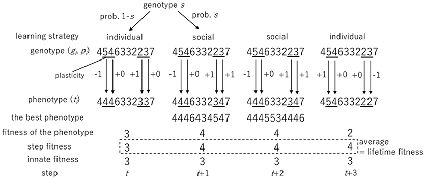
Figure 3. An example of learning process.
After completing L steps of learning, offspring grow up to parents and produce the offspring by the following genetic operations.
(1) The lifetime fitness of each individual is defined as the average step fitness over all the learning steps during its lifetime. Two parents are independently selected from the population by roulette wheel (fitness proportionate) selection based on the lifetime fitness.
(2) For GI and GP, we apply a single-point crossover operation on a pair of cloned chromosomes from the parents, which produce two offspring chromosomes for GI and GP, respectively.
(3) Each value of cloned genes gi, pi, s from the parents are mutated with the probabilities mg, mp, and ms, respectively. A mutation occurring in gi adds +1 or −1 to the current value, and if the value exceeds its domain, does it again until satisfying the condition. A mutation in pi flips the current binary value. A mutation in s adds a random value from a normal distribution N(0, σ2). If the value goes lower than 0, it also does it again until satisfying the condition.
We conducted computational experiments to explore the coevolution between individual and social learning, using the parameters shown in Table 3. The initial population was composed of N/2 individuals of which gi were all 1, and pi and s were randomly determined. We assumed two cases of experiments, one in which individuals were allowed to perform individual learning only, and the other in which the proportion of social learning could evolve (as described above). Experiments were conducted 20 times for each case, and the average lifetime fitness at the final generation of the former case was 6.91 and that of the latter was 8.98. Table 4 shows the breakdown of the dominant values of the fitness function in the last generation in the 20 trials for each case. The average fitness tends to be slightly smaller than dominant values of them in the population due to the deviation of the distribution. Thus, if the average lifetime fitness exceeded a certain value n−0.1, we regarded that it had reached n. In the former case, it reached 7 in all the trials, but in the latter case, it increased to 10 which is the highest value in this model, and in all experiments, it reached higher values than 7. Therefore, the social learning can facilitate the adaptive evolution of the population on a rugged fitness landscape.
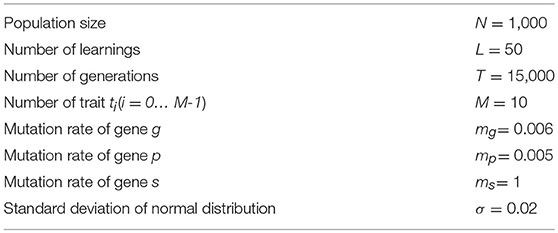
Table 3. Default parameter values.
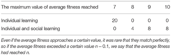
Table 4. Breakdown of the how much average fitness increased (Total 20).
First, we show the details of experiments only with individual learning. We fixed genes s of all individuals to 0. Figure 4 shows a result of the experiments, which indicates the typical dynamics of evolution process in this case. In the Figure 4A, the horizontal axis represents the generation. The green and red lines show the highest fitness and the average of the lifetime fitness, respectively. The blue line shows the average innate fitness, which represents the average fitness of initial phenotypic values gi. In the Figure 4B, the blue line shows the proportion of plastic phenotypes and the light blue line shows the average of the variances of gene gi in each locus. The red line shows the average plasticity contribution. We used the plasticity contribution in order to see how and when learning effectively worked. Specifically, as this index, we calculated the number of the learned trait (in the sense that it was changed from the initial trait) which contributed to the fitness (in the sense of Equations 1, 2) divided by the number of the plastic traits, in the most adaptive phenotype attained by the individual (that equals to the phenotype in the last learning step). Figure 4C represents the distribution of the innate fitness, and Figure 4D represents the distribution of calculated fitness by individual learning in learning steps and Figure 4E represents the enlarged view of Figure 4D.
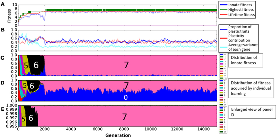
Figure 4. The evolution of the population with individual learning. (A) Shows the initial and highest and lifetime fitness, and (B) shows the proportion of plastic traits, plasticity contribution and average variance of each gene. (C) Shows the distribution of the innate fitness. (D) Shows the distribution of acquired step fitness by individual learning, and (E) shows the enlarged view of (D), when agents doing only individual learning.
We see from Figure 4A that individuals evolved through repeated occurrences of the two steps of Baldwin effect during the first 2200 generations. (1) The highest fitness increased (discovering adaptive traits by individual learning) and the average fitness increased while the average innate fitness remained steady or decreased (agents which can learn adaptive traits increased in population). This corresponds to the 1st step of Baldwin effect. (2) Then, the innate fitness increased (because of the learning failure cost, agents evolve to adaptive traits innately). This corresponds to the 2nd step of Baldwin effect. As a result, the average lifetime fitness increased to 7.0 until around the 2200th generations, and converged to this value, meaning that the population got stuck in the local optima of the rugged fitness landscape.
Figure 5 represents the enlarged view of Figure 4. Figure 5(1–4) illustrate typical phases of the evolution of the population on the rugged fitness landscape, each corresponding to the duration indicated by a double headed arrow. Each individual is represented as a pair of a circle, showing its innate fitness, and a square, showing its lifetime fitness. The circle and the square are connected with a directional arrow, representing its learning process. In general, individuals are classified into three types a, b, c. Thick circles and squires represent dominant individuals in the population. The string of numbers around each individual represents its example phenotypes. The underlined values are plastic traits.
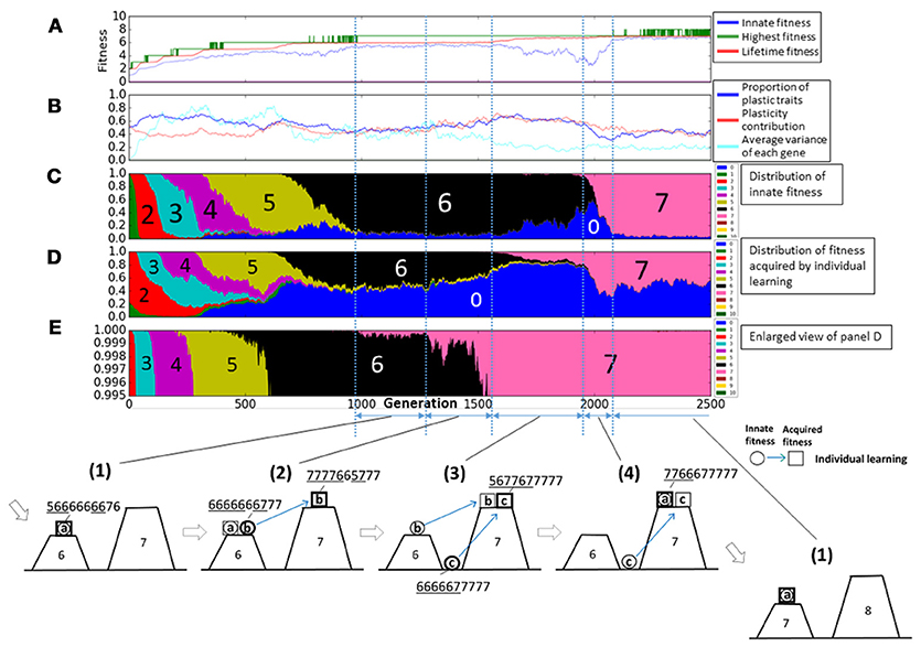
Figure 5. Enlarged view of Figure 4. (1–4) Illustrate typical phases of the evolution of the population on the rugged fitness landscape, each corresponds to the duration indicated by a double headed arrow. Each individual is represented as a pair of a circle, showing its innate fitness, and a square, showing its lifetime fitness. The circle and the square are connected with a directional arrow, representing its learning process. Thick circles and squares represent dominant individuals in the population.
First, in phase (1), most of agents, classified as type-a, had the same fitness values before and after learning, meaning that they stayed on a peak of the landscape through their lifetime. This corresponds to around 1000th to 1250th generation. We can see that most of agents had the fitness 6 innately from Figure 5C, and also in Figure 5D, few agents acquired the fitness 7 by learning. This is because they had few “7” traits and it was difficult to satisfy the condition num(7) ≥ 7 by learning.
In phase (2), individuals, classified as type-b, who had the higher lifetime fitness than the innate fitness increased in the population, meaning that they jumped over the valley of the fitness landscape by learning. This phase corresponds to around 1250th to 1500th generation. These individuals had more plastic traits than type-a individuals and also they had more “7” traits innately. As a result, they could satisfy the condition num(7) ≥ 7 by learning. We can see the proportion of plastic traits and plasticity contribution increased in Figure 5B. The increase of “7” traits in innate phenotypes decreased the probability of acquiring the fitness 6 by learning as shown in Figure 5D. In Figure 5E, we can confirm the proportion of fitness 7 acquired by learning increased.
In phase (3), individuals which were born in the valley of the fitness landscape but could reach the higher peak by learning increased. They are classified as type-c. This phase corresponds to around 1500th to 1900th generation in the graph. This is because individuals came to have more traits 7 innately to increase the probability of acquiring the fitness 7. As a result, they became to not to satisfy the condition num(n) ≥ n innately in any numbers and thus, their innate fitness became 0. We can see the proportion of the innate fitness 0 increased in Figure 5C and the proportion of fitness 7 acquired by learning increased in Figure 5D.
In phase (4), individuals who existed on the top of the higher peak increased. This phase corresponds to around 1900th to 2100th generation. They satisfied the condition num(7) ≥ 7 innately and they could not acquire more adaptive phenotypes by learning. Thus, they were type-a agents. In Figure 5C, the proportion of plastic traits decreased to around 0.3 because non-plastic traits of “7” traits increased the probability of acquiring fitness 7 phenotypes by learning. We can confirm the proportion of the innate fitness 7 increased in Figure 5C.
After phase (4), the population converged to the top of the peak of the fitness 7, and it means the evolution process got back to phase (1). The population climbed the rugged fitness landscape by repeating these 4 phases until around 2200th generation. However, as seen in Figure 5, the evolution process completely converged. This is because the population could not acquire the fitness 8 stably as shown by the repeated temporal increase of the highest fitness in Figure 5A.
Next, we show the details of experiments with social learning. Figure 6 shows a typical example when the average fitness increased to 10. This is a universal behavior in every experiments when fitness increased. The representation is the same as in Figure 4, but it is changed in some points. In Figure 6A, highest fitness is replaced by that acquired by individual learning (green line) and that acquired by social learning (purple line). If they took the same values, they are represented by black line. In Figure 6B, the proportion of social learning is added, and in Figure 6F, the proportion of fitness acquired by social learning is added. In this model, population finally reached the fitness 10, the maximum value of this fitness function.
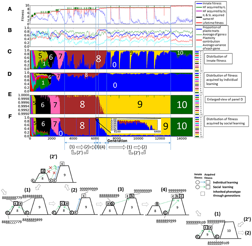
Figure 6. The evolution of the population with individual and social learning. (A) Shows the initial and highest and lifetime fitness, and (B) shows the proportion of plastic traits, plasticity contribution and average variance of each gene. (C) Shows the distribution of the innate fitness. (D) Shows the distribution of acquired step fitness by individual learning, and (E) shows the enlarged view of (D). (F) Shows the distribution of acquired step fitness by social learning. (1–4) illustrate typical phases of the evolution of the population on the rugged fitness landscape, each corresponds to the duration indicated by a double headed arrow. Each individual is represented as a pair of a circle, showing its innate fitness, and a square showing its lifetime fitness. The dotted square showing inherited phenotypes through generations. The circle and the square are connected with a directional arrow, representing its learning process. Blue arrow represents individual learning and green arrow represents social learning. Thick circles and squares represent dominant individuals in the population.
The gene s, which is the probability of social learning, evolved to high values at early generation, and it kept high values. This is because imitating phenotypes of the best agents was more adaptive than acquiring adaptive phenotypes by trial and error. It took high values more stably as the lifetime fitness increased. This is because as the fitness landscape became more rugged, acquiring adaptive phenotypes by individual learning became more difficult. In addition, once such adaptive phenotypes were acquired by individual learning and then came to be maintained in the population by social learning, social learning became more adaptive than individual learning.
This adaptive evolution process was caused by complex interactions between individual learning and social learning. Figure 6(1–4) illustrate typical phases of the evolution of the population on the rugged fitness landscape as in Figure 4. A green directional arrow, which connects a circle and a square, represents a change in the fitness by social learning, and a dotted square represents the best phenotypes shared in the population through imitation from parent individuals to offspring individuals in the population.
First, in phase (1), most of agents, classified as type-c, acquired adaptive, but innately non-adaptive, phenotypes by social learning. They had almost the same lifetime fitness as type-a agents, so they can coexist with them and the genetic diversity increased.
In phase (2), because of the increased genetic diversity due to social learning, some type-c individuals occasionally had higher numbered values of innate phenotypes, meaning that they were born in the valley near to the higher peak of fitness landscape. They could found new adaptive phenotypes by individual learning, and became the best individuals to be imitated by others.
However, other type-c individuals often failed to imitate such new adaptive phenotypes mainly due to the lack of plasticity as illustrated in Figure 6(2′). This made the population lose the adaptive phenotypes and type-a individuals dominated the population again. Thus, the population went back to phase (1). These transition processes repeatedly occurred from around 3200th to 6000th generation in this trial. The phases Figure 6(1–2′) correspond to the increase in the innate fitness 0 in Figure 6C, the increase in the acquired fitness 9 in Figure 6E, and the increase in the innate fitness 8, respectively.
On the other hand, once individuals successfully imitated the new adaptive phenotypes by social learning and they were maintained in the population, type-b individuals, who could acquire such new adaptive phenotypes while keeping innate adaptive phenotypes, increased in the population, as illustrated in Figure 6(3). This phase corresponds to around 6000th to 6300th generation. We can see from the enlarged view in Figure 6F, which is marked by a square, individuals which could imitate fitness 9 phenotypes increased slightly. This phase is the similar to phase (2) in the case with individual learning only.
In phase (4), type-c individuals, who could acquire new adaptive phenotypes more quickly by discarding innate adaptive phenotypes, increased in the population as in phase (3) in the case with individual learning only. This phase corresponds to around 6300th to 7000th generation. The proportion of plastic traits and plasticity contribution in Figure 6B took very high values around 0.9 compared with those in the case with individual learning only. It means that individuals highly relied on social learning and they need high plasticity to imitate precisely. In Figure 6B, the average variance of each gene increased and it shows type-c individuals increased in the population.
Finally, the evolution process went back to phase (1) but the population existed on a more adaptive peak. Type-c individuals appeared in the other side of the valley and dominated the population, and a few type-a individuals appeared. Therefore, the evolutionally process was cyclic, and individuals evolved through this process on the rugged fitness landscape.
In addition, we conducted experiments with different settings of parameters, and found that the basic scenario of evolution process did not change under the assumption of plausible parameter settings. We also found that some parameters can affect the speed of evolution (i.e., the fitness increase). For example, the larger number of learning iterations L, which is a parameter relating to learning process, can increase the speed of evolution, which is expected to be due to the increase in chances to acquire new and adaptive phenotypes, and vice versa. On the other hand, the higher values of parameters on mutation process mg, mp, ms, and σ generally decreased the speed of evolution if they were increased. These are mainly due to the fact that a strong mutation prevents the population from keeping adaptive sets of genotypes, plasticity, and high social learning rate. But the lower mg also slowed down the speed of evolution because of the smaller genetic diversity.
We constructed a computational evolutionary model with individuals that can learn individually or socially on a multi-modal fitness landscape as a more realistic situation than those which have been used in previous research. Comparing the results with only individual learning and with both of learning, we found essential differences between these two learning, which can be described at more general level as follows.
In general, learning has an effect to expand the individuals' search range in phenotypic space. At the same time, it also enables individuals which have different genotypes to have similar phenotypes and fitness values, which means that, at the population level, learning has an effect of bringing the population genetic diversity. Comparing individual and social learning, the characteristic of individual learning is the ability to find new adaptive phenotypes, which cannot be achieved by social learning. On the other hand, social learning has greater amount of the above-described effects of learning, especially of an increase in genetic diversity, by allowing individuals to imitate the adaptive phenotype in population already found by individual learning, without trial and error.
Based on these differences, individual and social learning work complementarily in the course of adaptive evolution on the rugged fitness landscape as follows. Individual learning can find new adaptive phenotypes thanks to the diversity of genetic expressions created by social learning. It is illustrated in the transition from Figure 5(1) in which individuals that were born on the valleys on either side of a peak (8) leach the peak by social learning to Figure 5(2) in which an individual that was born on the valley of the right side of the top found a new fitness peak (9) by individual learning. On the other hand, social learning can keep a new adaptive phenotype found by individual learning in the population. It is illustrated in the transition from Figures 5(2,3) in which individuals on the lower peak (8) can find the higher peak (9) by social learning, thus keeping the new peak found by individual learning in the population. However, if every social learning is unsuccessful because of keeping different values for non-plastic trait, the peak found by individual learning is lost and the population moves back to Figure(1) via Figure(2′).
We have described how individual and social learning interact with each other and how it enables individuals to find adaptive phenotypes on the rugged fitness landscape with valleys which cannot be crossed by individual learning alone. In recent years, theoretical and empirical research to predict and explain social learning strategies of humans and other animals has been conducted [16]. One of the promising direction would be to introduce several typical strategies for social learning into the model and investigate the effect of the interaction between the strategies on the evolutionary scenario of the cooperation. It is also would be the future direction to consider network structures of social interactions so as to make the model more realistic, in terms of the “whom” aspect of social learning.
MH, RS, and TA designed the experimental procedures, conducted experiments, analyzed the results, and wrote the manuscript.
This work was supported by MEXT/JSPS KAKENHI Grant Number JP17H06383 in #4903 (Evolinguistics), JP15K00335, JP15K00304, and JP18K11467.
The authors declare that the research was conducted in the absence of any commercial or financial relationships that could be construed as a potential conflict of interest.
2. Turney P, Whitley D, Anderson RW. Evolution, learning, and instinct: 100 years of the Baldwin effect. Evol Comp. (2007) 4:4–8. doi: 10.1162/evco.1996.4.3.iv
4. Rendell L, Fogarty L, Laland KN. Rogers' paradox recast and resolved: population structure and the evolution of social learning strategies. Evolution (2010) 64:534–48. doi: 10.1111/j.1558-5646.2009.00817.x
5. Jones D, Blackwell T. Social learning and evolution in a structured environment. In: Proceedings of the Eleventh European Conference on the Synthesis and Simulation of Living Systems (ECAL2011) (Paris) (2011). p. 380–8.
6. Tamura K, Kobayashi Y, Ihara Y. Evolution of individual versus social learning on social networks. J R Soc Interface. (2015) 12:1–9. doi: 10.1098/rsif.2014.1285
7. Kobayashi Y, Wakano JY. Evolution of social versus individual learning in an infinite island model. Evolution. (2012) 66:1624–35. doi: 10.1111/j.1558-5646.2011.01541.x
9. Enquist M, Eriksson K, Ghirlanda S. Critical social learning: a solution to Rogers's paradox of nonadaptive culture. Am Anthropol. (2007) 109:727–34. doi: 10.1525/aa.2007.109.4.727
10. Mesoudi A. An experimental simulation of the “copy-successful-individuals” cultural learning strategy: adaptive landscapes, producer–scrounger dynamics, and informational access costs. Evol Hum Behav. (2008) 29:350–63. doi: 10.1016/j.evolhumbehav.2008.04.005
11. Boyd R, Richerson PJ. Culture and the Evolutionary Process. Chicago, IL: University of Chicago press (1985).
12. Henrich J, Boyd R. The evolution of conformist transmission and the emergence of between-group differences. Evol Hum Behav. (1998) 19:215–41.
13. Wakano JY, Aoki K. (2007). Do social learning and conformist bias coevolve? Henrich and Boyd revisited. Theor. Popul. Biol. 72. 504–12. doi: 10.1016/j.tpb.2007.04.003
14. Nakahashi W, Wakano JY, Henrich J. Adaptive social learning strategies in temporally and spatially varying environments. Hum Nat. (2012) 23:386–418. doi: 10.1007/s12110-012-9151-y
15. Suzuki R, Arita T. Repeated occurrences of the Baldwin effect can guide evolution on rugged fitness landscapes. In: Proceedings of the First IEEE Symposium on Artificial Life (IEEE-Alife'07) (Honolulu) (2007). pp. 8–14.
Keywords: social learning, individual learning, coevolution, baldwin effect, fitness landscape
Citation: Higashi M, Suzuki R and Arita T (2018) The Role of Social Learning in the Evolution on a Rugged Fitness Landscape. Front. Phys. 6:88. doi: 10.3389/fphy.2018.00088
Received: 20 November 2017; Accepted: 23 July 2018;
Published: 28 August 2018.
Edited by:
Tatsuya Sasaki, F-Power Inc., JapanReviewed by:
Eduardo J. Izquierdo, Indiana University Bloomington, United StatesCopyright © 2018 Higashi, Suzuki and Arita. This is an open-access article distributed under the terms of the Creative Commons Attribution License (CC BY). The use, distribution or reproduction in other forums is permitted, provided the original author(s) and the copyright owner(s) are credited and that the original publication in this journal is cited, in accordance with accepted academic practice. No use, distribution or reproduction is permitted which does not comply with these terms.
*Correspondence: Masahiko Higashi, aGlnYXNoaUBhbGlmZS5jcy5pcy5uYWdveWEtdS5hYy5qcA==
Disclaimer: All claims expressed in this article are solely those of the authors and do not necessarily represent those of their affiliated organizations, or those of the publisher, the editors and the reviewers. Any product that may be evaluated in this article or claim that may be made by its manufacturer is not guaranteed or endorsed by the publisher.
Research integrity at Frontiers
Learn more about the work of our research integrity team to safeguard the quality of each article we publish.