A Renormalization Group Procedure for Fiber Bundle Models

We introduce two versions of a renormalization group scheme for the equal load sharing fiber bundle model. The renormalization group is based on formulating the fiber bundle model in the language of damage mechanics. A central concept is the work performed on the fiber bundle to produce a given damage. The renormalization group conserves this work. In the first version of the renormalization group, we take advantage of ordering the strength of the individual fibers. This procedure, which is the simpler one, cannot be generalized to other fiber bundle models such as the local load sharing one. The second renormalization group scheme based on the physical location of the individual fibers may be generalized to other fiber bundle models.

1. Introduction

In an age where computer modeling of fracture and material breakdown is reaching a stage where the systems one may study span from the atomistic level to the continuum level in a single go [1, 2], one may wonder what is the use of simplified models. The fact is that such modeling is more important than ever. The experimental approach tells us what Nature dictates the systems to do. The computational approach tells us what would happen if we, and not Nature, made the rules. With the computational approach we are able to know exactly what every single atom in the material is doing. However, this is not equivalent to understanding what is happening. For this, we need to find the underlying principles, and this is where the need for simplified models come in.

Looking back in history, the study of equilibrium critical phenomena became “well understood” in the late seventies. Central to conquest of this field was the Ising spin model [3, 4]. It is hard to imagine how the deep understanding of the nature of critical phenomena could have evolved without the guidance of this model and all its more complex relatives.

There are similarities between equilibrium phenomena and fracture, but also large differences. The similarities come from the development of long-range correlations as the fracture process proceeds in the same way as such correlations develop when approaching a critical point. On the other hand, whereas parameters need to be adjusted to approach criticality in equilibrium systems, in fracture the system approaches this state without the tuning of parameters. The correlations that develop during the fracture process stem from the way the stress field develops. However, they also reflect themselves in e.g., the spatial correlations in the post mortem fracture surfaces [5, 6].

The fiber bundle model [7, 8] is a model that plays somewhat the same role with respect to fracture phenomena as the Ising model plays with respect to equilibrium critical phenomena [9, 10]. In its simplest form, the Equal Load Sharing (ELS) version, it consists of N parallel fibers of length L placed between two parallel stiff clamps a distance L+Δ apart. Each fiber responds linearly with a force f to the load Δ,

$\begin{array}{rc}f=\kappa \Delta ,& (1)\end{array}$

where κ is the spring constant. κ is the same for all fibers. Each fiber has a load threshold t assigned to it. The load thresholds are drawn randomly from a probability density p(t). If the load Δ exceeds this threshold, the fiber fails irreversibly. The total load on the fiber bundle is

$\begin{array}{rc}F=\kappa (N-n)\Delta & (2)\end{array}$

when n fibers have failed. This means that all thresholds t ≤ Δ have failed.

It is the aim of this paper to construct a real-space renormalization group scheme [11] for the ELS fiber bundle model. We hope, the renormalization group scheme is generalizable to more complex fiber bundle models such as the Local Load Sharing (LLS) fiber bundle model [12] or the Soft Clamp (SC) fiber bundle model [13].

Our goal is to construct a mapping from a fiber bundle containing N fibers to a fiber bundle containing N′ = N/2 fibers in such a way that the variables describing the entire fiber bundle, such as F and Δ remain unaltered. This we do by replacing the fibers characterized by a spring constant κ and threshold distribution p(t) by a new set of fibers characterized by a spring constant κ′ and a threshold distribution p′(t).

In order to construct the real space renormalization group, it is necessary to formulate the ELS fiber bundle model within damage mechanics [14–16]. We present in section 2 a new formulation of the ELS fiber bundle model within such a framework tailored for the renormalization group formulation to be presented.

It is an important feature of the ELS fiber bundle model that it is infinite dimensional. That is, all fibers interact with all other fibers in exactly the same way. This is in contrast to e.g., the soft clamp fiber bundle model where the closer two fibers are, the more they interact.

Hence, when we in the renormalization group scheme to be presented choose to replace pairs of fibers by a single fiber by going from N to N/2 fibers, we may choose to group them together as we like. We explore this property in section 3.1 where fibers are grouped together in terms of increasing strength t. This vastly simplifies the construction of the renormalization group scheme.

However, if the renormalization group scheme we present is to have any bearing on the more complex fiber bundle models such as the LLS and the SC models where the relative position of the fibers do matter, the renormalization group presented in section 3.1 is useless. Hence, in section 3.2, we present the real space renormalization group scheme. We map out the flow in parameter space and the fixed point structure.

In section 4 we consider how the strength of the fiber bundle evolves under the renormalization group scheme.

The last section 5 contains a discussion of our results.

2. Fiber Bundle Model in a Damage Mechanics Formulation

We will in this section formulate the equal load sharing model in a damage mechanics formulation based on energetic considerations. Damage mechanics is an approach to fracture in the continuum limit where the fractures are represented by a continuous damage parameter. Abaimov [15] and Berthier [16] present some damage mechanics formulations of the ELS fiber bundle model. Our approach is different from both of them.

When the fiber bundle is loaded, the fibers fail according to their thresholds, the weaker before the stronger. We suppose that n fibers have failed. At a load Δ, the fiber bundle carries a force

$\begin{array}{rc}F=N\kappa (1-d)\Delta ,& (3)\end{array}$

where we have defined the damage

$\begin{array}{rc}d=\frac{n}{N}& (4)\end{array}$

and used Equation (2). The damage parameter d becomes continuous as N → ∞.

A fundamental equation in what follows is the relation between damage d and the threshold of the weakest surviving fiber, τ. Since the fibers fail in a sequence ordered from the weakest to the strongest, we have that

$\begin{array}{rc}d=P(\tau ),& (5)\end{array}$

where the cumulative probability distribution corresponding to the threshold distribution p(t) is given by

$\begin{array}{rc}P(t)={\displaystyle \underset{0}{\overset{t}{\int }}}d{t}^{\prime }p(t^{\prime }).& (6)\end{array}$

The cumulative probability gives the probability to find a threshold smaller than or equal to t. We will assume first that the load Δ is our control parameter. Afterwards, we will assume that the force carried by the fiber bundle F is our control parameter. We now construct the energy budget according to damage mechanics. At a load Δ and damage d, the elastic energy stored by the surviving fibers is

$\begin{array}{rc}{E}^e(\Delta ,d)=\frac{N\kappa }{2}{\Delta }^2(1-d).& (7)\end{array}$

We are here assuming the limit N → ∞ and κ → 0 so that the product Nκ remains constant.

The energy dissipated by the failed fibers is given by

$\begin{array}{rc}{E}^d(d)=\frac{N\kappa }{2}{\displaystyle \underset{0}{\overset{d}{\int }}}d\delta {\left[P^{-1}(\delta )\right]}^2.& (8)\end{array}$

The work performed on the system to reach the state (Δ, d) from the state (0, 0) is thus,

$\begin{array}{l}W(\Delta ,d)=E^e(\Delta ,d)+E^d(d)\\ =\frac{N\kappa }{2}\left[{\Delta }^2(1-d)+{\displaystyle {\int }_0^{d}d\delta {[P^{-1}(\delta )]}^2}\right].& (9)\end{array}$

The force conjugated to the load Δ is

$\begin{array}{rc}F={\left(\frac{\partial W}{\partial \Delta }\right)}_d=N\kappa \Delta (1-d),& (10)\end{array}$

which is identical Equation (3), as it must.

The damage driving force ${F}$ conjugate to the damage d is

$\begin{array}{ll}F=-{\left(\frac{\partial W}{\partial d}\right)}_{\Delta }=\frac{N\kappa }{2}\left[{\Delta }^2-{\left[P^{-1}(d)\right]}^2\right],& (11)\end{array}$

and the equilibrium condition is

$\begin{array}{ll}F=0,& (12)\end{array}$

which when combined with Equation (11) gives

$\begin{array}{rc}\Delta =P^{-1}(d).& (13)\end{array}$

This equation is equivalent to Equation (5) when t = Δ and it simply states that at a load Δ all fibers with threshold less than or equal to it have failed.

We now turn to controlling the force F rather than the load Δ. Using Equation (3), we have

$\begin{array}{rc}\Delta (F)=\frac{F}{N\kappa }\frac{1}{1-d}.& (14)\end{array}$

The corresponding work we find via the Legendre transform,

$\begin{array}{rc}U(F,d)=W(\Delta (F),d)-F\Delta (F).& (15)\end{array}$

Combining this equation with Equations (9, 14) we find

$\begin{array}{rc}U(F,d)=-\frac{F^2}{2N\kappa }\frac{1}{1-d}+\frac{N\kappa }{2}{\displaystyle \underset{0}{\overset{d}{\int }}}d\delta {\left[P^{-1}(\delta )\right]}^2.& (16)\end{array}$

We calculate the damage driving force

$\begin{array}{ll}F=-{\left(\frac{\partial U}{\partial d}\right)}_F=\frac{F^2}{2N\kappa }\frac{1}{{(1-d)}^2}-\frac{N\kappa }{2}{[P^{-1}(d)]}^2.& (17)\end{array}$

The equilibrium condition Equation(12) gives

$\begin{array}{rc}F=N\kappa (1-d)P^{-1}(d).& (18)\end{array}$

Equation (18) when combined with Equation (5) gives

$\begin{array}{rc}F=N\kappa \left[1-P(\Delta (F))\right]\Delta (F),& (19)\end{array}$

which is the force-load characteristics of the fiber bundle model. This equation is usually derived using order statistics. We see that the derivation using damage mechanics leads to the same result.

It is interesting to note that the equilibrium condition (Equation 12) can only be satisfied for

$\begin{array}{rc}\frac{F}{N\kappa }\le {\displaystyle \underset{d}{max}}(1-d)P^{-1}(d).& (20)\end{array}$

If F exceeds this limit, ${F}$ is positive and catastrophic failure ensues.

3. Renormalization Group

The renormalization group transformation that we are about to construct will consist of replacing the original fiber bundle containing N individual fibers by a new fiber bundle containing N/2 individual fibers. We introduced the damage parameter d = n/N in Equation (4), where n is the number of failed fibers. It is only in the limit N → ∞ that d is a continuous parameter. It is convenient in the following to use the notation d(n, N) = n/N in order to indicate that for finite N, d(n, N) is a discrete variable. We note the following equality,

$\begin{array}{rc}d(n,N)=d\left(\frac{n}{2},\frac{N}{2}\right).& (21)\end{array}$

We now demand that the total work performed on the system, Equation (9), is kept constant by the renormalization group transformation. That is, we have

$\begin{array}{rc}{W}_N(\Delta ,d(n,N))=W_{N/2}\left(\Delta ,d\left(\frac{n}{2},\frac{N}{2}\right)\right).& (22)\end{array}$

As we are here assuming N to be finite, we have explicitly introduced it as a parameter in writing W→W_N. Equation (22) is central in what follows. As the number of individual fibers is reduced from N to N/2, the possible values that the damage parameter d(n, N) can take is also reduced by a factor 2. However, for those values of the damage parameter that remain, the energy is unchanged.

We have just stated that the energy (Equation 9) is to remain constant under the transformation. The energy consists of two parts, $W_N=E_N^e+E_N^d$, see Equations (7, 8). In order to fulfill Equation (22), the elastic energy $E_N^e$ and the energy dissipated by the damage $E_N^d$ each needs to be constant under the renormalization group transition.

In order for the elastic energy to be constant under the renormalization group transformation, we need to transform the elastic constant. The elastic energy will be constant if keep the load Δ fixed, i.e.,

$\begin{array}{rc}\Delta \to {\Delta }^{\prime }=\Delta ,& (23)\end{array}$

and we set

$\begin{array}{rc}\kappa \to {\kappa }^{\prime }=2\kappa & (24)\end{array}$

so that

$\begin{array}{rc}N\kappa =\left[\frac{N}{2}\right]\left[2\kappa \right],& (25)\end{array}$

when

$\begin{array}{rc}N\to N^{\prime }=\frac{N}{2}.& (26)\end{array}$

We keep the load Δ fixed during the transformation.

The energy dissipated by the failed fibers, $E_N^d$, is constant under the renormalization group transformation if, in the limit N → ∞, we have

$\begin{array}{l}{E}_N^d=\frac{N\kappa }{2}{\displaystyle {\int }_0^{d(n,N)}d\delta {\left[P^{-1}(\delta )\right]}^2}\\ =\frac{\left(N/2\right)\left(2\kappa \right)}{2}{\displaystyle {\int }_0^{d(n/2,N/2)}d\delta {\left[P^{-1}(\delta )\right]}^2.}& (27)\end{array}$

When N is finite, Equation (27) becomes

$\begin{array}{rc}\frac{\kappa }{2}{\displaystyle \sum _{i=1}^n}{t}_{(i)}^2=\frac{2\kappa }{2}{\displaystyle \sum _{j=1}^{n/2}}{t^{\prime }}_{(j)}^2,& (28)\end{array}$

where we have ordered the thresholds, t₍₁₎ ≤ t₍₂₎ ≤ ⋯ ≤ t_(N−1) ≤ t_(N) and ${t^{\prime }}_{(1)}\le {t^{\prime }}_{(2)}\le \cdots \le {t^{\prime }}_{(N/2-1)}\le {t^{\prime }}_{(N/2)}$.

These ordered thresholds are averaged over an ensemble. That is, we have M samples. The kth largest threshold in sample m is $t_{(k)}^m$, and we have

$\begin{array}{rc}{t}_{(k)}=\frac{1}{M}{\displaystyle \sum _{m=1}^M}{t}_{(k)}^m.& (29)\end{array}$

A fundamental result in order statistics is that the average frequency of the kth ordered threshold is given by

$\begin{array}{rc}P(t_{(k)})=\frac{k}{N+1},& (30)\end{array}$

in the limit when M → ∞, see Gumbel [17].

In order to complete the renormalization group transformation, we need to define the threshold transformation

$\begin{array}{l}\left\{t_{(1)},t_{(2)},\dots ,t_{(N-1)},t_{(N)}\right\}\to \\ \left\{{t^{\prime }}_{(1)},{t^{\prime }}_{(2)},\dots ,{t^{\prime }}_{(N/2-1)},{t^{\prime }}_{(N/2)}\right\}& (31)\end{array}$

so that Equation (28) is fulfilled. There is no unique way to do this. We will in the following present two different transformations. The first one, which we call the order space transformation, consists of grouping the initial thresholds according to their value. The second one, the real space transformation, consists of grouping the initial thresholds according to their location.

3.1. Renormalization Group in Order Space

We write the sum in Equation (28) as

$\begin{array}{rc}{\displaystyle \sum _{i=1}^n}{t}_{(i)}^2=2{\displaystyle \sum _{j=1}^{n/2}}\left[\frac{t_{(2j-1)}^2+t_{(2j)}^2}{2}\right]=2{\displaystyle \sum _{j=1}^{n/2}}{t^{\prime }}_{(j)}^2.& (32)\end{array}$

Hence, we define the order space threshold transformation at the indivdual sample level as

$\begin{array}{rc}{t}_{(i)}^m\to {t^{\prime }}_{(j)}^m={\left[\frac{{(t_{(2j-1)}^m)}^2+{(t_{(2j)}^m)}^2}{2}\right]}^{1/2},& (33)\end{array}$

where as in Equation (29) the index m identifies the sample.

Equations (23, 24, 26, and 33) define the order space renormalization group transformation, fulfilling Equation (22).

Using Equation (30), we have

$\begin{array}{rc}P(t_{(2j-1)})=P(t_{(2j)})-\frac{1}{N},& (34)\end{array}$

when N≫1. To first order in 1/N, this gives

$\begin{array}{rc}{t}_{(2j-1)}=t_{(2j)}-\frac{1}{Np(t_{(2j)})}.& (35)\end{array}$

Combining this expression with renormalization group transformation Equation (33), gives

$\begin{array}{rc}{t^{\prime }}_{(j)}=t_{(2j)}-\frac{1}{2Np(t_{(2j)})},& (36)\end{array}$

where ${t^{\prime }}_{(j)}$ is the jth smallest average threshold out of N/2 and t_(2j) is the 2jth average threshold out of N. Hence, for large N, any threshold distribution p(t) will be invariant under this renormalization group transformation.

We show in Figure 1, the evolution of the distribution of individual thresholds of M = 10⁶ samples, each having N = 2¹² fibers, as we reiterate the order space renormalization group transformation. The N = 2¹² thresholds for the initial system were generated from a flat distribution on the unit interval. As we see from the figure, the distribution does not change as the renormalization group transformation is iterated. In fact, the formulation in Equations (32–36) are quite general in nature and the results should not depend on the type of thresold distribution. We have produced numerical results (Figure 2) for a non-uniform thresold distribution with the power-law type form p(t) = (1+α)t^α, with α = 1. It is clear from Figure 2 that the non-uniform threshold distribution also remains invariant under the renormalization group transformation.

FIGURE 1

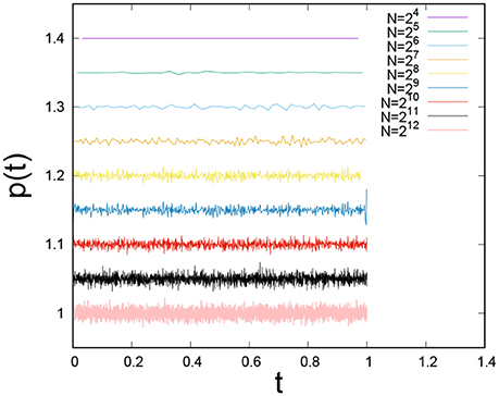
Figure 1. Evolution of threshold distribution for M = 10⁶ fiber bundles, each containing N = 2¹² fibers when repeating the order space renormalization group transformation. The initial threshold distribution was uniform on the unit interval. We have added a constant factor to p(t) for each iteration of the renormalization group in order to separate them.

FIGURE 2

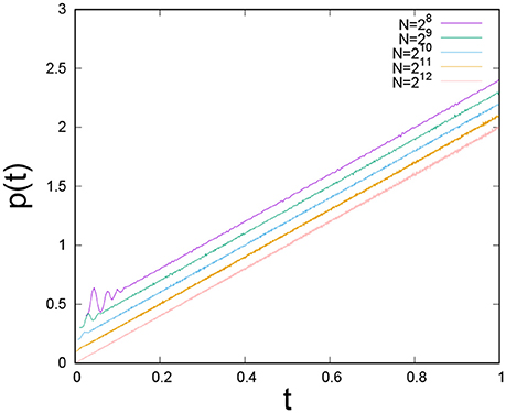
Figure 2. Evolution of threshold distribution for M = 10⁴ fiber bundles, each containing N = 2¹² fibers when repeating the order space renormalization group transformation. The initial threshold distribution was non-uniform (linearly increasing) on the unit interval. We have added a constant factor to p(t) for each iteration of the renormalization group in order to separate them.

The renormalization group transformation in terms of the parameters of the model, Equations (23), (24), and (33), defines the flow in parameters space,

$\begin{array}{ll}\left(\begin{array}{c}\Delta \\ \kappa \\ d\end{array}\right)\to \left(\begin{array}{c}\begin{array}{c}{\Delta }^{\prime }\\ {\kappa }^{\prime }\\ d^{\prime }\end{array}\end{array}\right).& (37)\end{array}$

We will now study the flow of the parameters (Δ, κ, d) under the renormalization group.

For the uniform distribution on the unit interval, i.e., P(t) = t, the work Equation (9) is

$\begin{array}{rc}{W}_N(\Delta ,d)=\frac{N\kappa }{2}\left[{\Delta }^2(1-d)+\frac{d^3}{3}\right].& (38)\end{array}$

We will in the following assume this threshold distribution for simplicity.

We assume that N is finite. Let us define a strain Δ_N(n) such that if Δ>Δ_N(n), at least n fibers have failed when the bundle is in equilibrium whereas if Δ < Δ_N(n), up to n−1 fiber have failed when the bundle is in equilibrium. We calculate the value of Δ_N(n) by demanding continuity,

$\begin{array}{l}\underset{\delta \to 0}{\lim }{W}_N\left({\Delta }_N(n)+\delta ,\frac{n}{N}\right)\\ =\underset{\delta \to 0}{\lim }{W}_N\left({\Delta }_N(n)-\delta ,\frac{n-1}{N}\right),& (39)\end{array}$

which for the uniform distribution on the unit interval gives

$\begin{array}{rc}{\Delta }_N(n)=\frac{\sqrt{1-3n+3n^2}}{\sqrt{3}N}.& (40)\end{array}$

For a given load Δ, we then have

$\begin{array}{rc}\cdots <{\Delta }_N(n-1)\le \Delta \le {\Delta }_N(n)<{\Delta }_N(n+1)<\dots ,& (41)\end{array}$

giving rise to the flow diagram shown in Figure 3, which is a projection into the (κ, d) plane of the flow Equation (37). For each iteration where N→N/2 and κ → 2κ, the position of Δ in the sequence of inequalities Equation (41) determines the damage level.

FIGURE 3

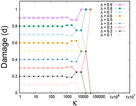
Figure 3. Flow in parameter space under the renormalization group transformation (37) projected onto the (κ, d) plane. The initial number of fibers was N = 2¹⁵, and the data are averaged over 10⁶ samples. The renormalization group is iterated 15 times so that the last bundle contains one fiber. The threshold distribution was uniform on the unit interval.

We show in Figure 4 the force-load curve for each renormalization group iteration. For each iteration, there is load ${\Delta }_N^c$ for which the force F is maximal. This maximum occurs for

$\begin{array}{ll}n=\{\begin{array}{ll}1\hfill & \text{if\hspace{0.17em}}N=1\hfill \\ \frac{N}{2}+1\hfill & \text{if\hspace{0.17em}}N=2,4,\cdots .\hfill \end{array}& (42)\end{array}$

FIGURE 4

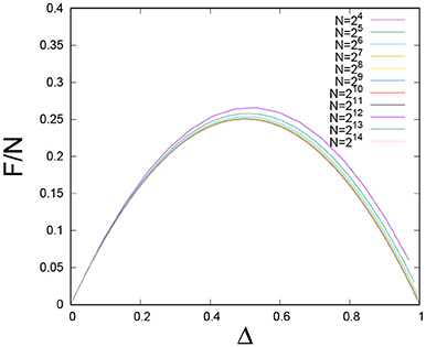
Figure 4. The force-load curve as we iterate the order-space renormalization group. The initial number of fibers was N = 2¹⁵ and the uniform distribution on the unit interval was assumed. Averages were taken over 10⁶ samples.

Combined with Equation (40), this gives

${\Delta }_N^c=\{\begin{array}{ll}\frac{1}{\sqrt{3}}\hfill & \text{if }N=1,\hfill \\ \frac{1}{2N}{\left[\frac{4}{3}+N(N+2)\right]}^{1/2}\hfill & \text{if }N=2,4,\cdots ,\hfill & (43)\end{array}$

and the corresponding peak stress is

$\frac{F_N^c}{N}=\{\begin{array}{ll}\kappa {\Delta }_N^c\hfill & \text{if }N=1,\hfill \\ \frac{\kappa {\Delta }_N^c}{2}\hfill & \begin{array}{l}\text{if }N=2,4,\cdots .\hfill \end{array}\hfill & (44)\end{array}$

This is illustrated in Figure 5.

FIGURE 5

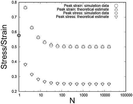
Figure 5. ${\Delta }_N^c$ and the corresponding force $F_N^c/N$ as we iterate the order-space renormalization group. The initial number of fibers was N = 2¹⁵ and the uniform distribution on the unit interval was assumed. Averages were taken over 10⁶ samples.

3.2. Renormalization Group in Real Space

The order space renormalization group we have defined and explored in section 3.1 is tailored for the ELS fiber bundle model since the physical position of the fibers do not matter. Hence, for the renormalization group procedure to be generalizable to more complex models than the ELS fiber bundle model, the LLS fiber bundle model being an example, we group neighboring fibers together.

We assume the fibers to be placed along a one-dimensional line. They are numbered from 1 to N. Hence, we are considering a one-dimensional system. The procedure that we describe is straight forward to generalize to e.g., having the fibers positioned at the nodes of a square lattice.

We follow the same procedure as for the order space renormalization group except that the group together of pairs of fibers are now in real space rather than in order space. Fiber number i has a threshold t_i. The renormalization group transformation of the thresholds then becomes

$\begin{array}{rc}{t}_{(i)}^m\to {t^{\prime }}_j^m={\left[\frac{{(t_{2j-1}^m)}^2+{(t_{2j}^m)}^2}{2}\right]}^{1/2}& (45)\end{array}$

at the individual sample level. As in the order space renormalization group, the work performed on the fiber bundle is conserved, see Equation (22). For an N = 2 fiber bundle, the order and real space renormalization groups are identical. Hence, we may see the real space renormalization group as Equation (1) grouping neighboring fibers into fiber bundles of size N = 2 and Equation (2) do an order space renormalization group iteration on each pair of fibers.

In contrast to the order space renormalization group, the threshold distribution is not invariant under the real space renormalization group. We show the evolution of the uniform distribution on the unit interval in Figures 6, 7. In Figure 6 we show the cumulative probability P(t) as it evolves (lines represent the P(t) values for different renormalization steps) from the initial P(t) = t. We note that all the iterated cumulative probabilities pass through the same point [t_c, P(t_c)]. In Figure 7, showing the evolution of the threshold distribution, we see that the threshold distribution is becoming increasingly peaked around t_c. Since the work is conserved as for the order space renormalization group, we will have that ${\Delta }_1(1)=1/\sqrt{3}$ also in this case. Since the threshold distribution is no longer invariant under the renormalization group, but approaches a delta function, we must have that $t_c=1/\sqrt{3}$. We can calculate the fixed point value $t_c=1/\sqrt{3}$ through the following argument, which is valid both for order and space renormalization group schemes: The final single fiber must have a strength which can conserve the energy of the whole bundle (with N fibers) we started with. From the energy conservation, we can write for an uniform distribution of fiber thresholds within (0, 1)

$\begin{array}{rc}\frac{1}{2}N\kappa t_c^2=\frac{1}{2}N\kappa {\displaystyle \underset{0}{\overset{1}{\int }}}{t}^{2}p(t)dt;& (46)\end{array}$

FIGURE 6

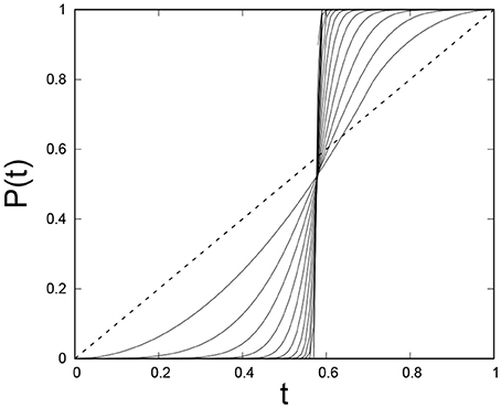
Figure 6. Evolution of the cumulative threshold probability under the real space renormalization group iteration is shown where lines represent the P(t) values for different renormalization steps. The initial number of fibers was N = 2¹⁵. A uniform threshold distribution on the unit interval is assumed, so that the cumulative probability is P(t) = t (dotted line) at the initial stage. Averages are taken over 10⁶ samples.

FIGURE 7

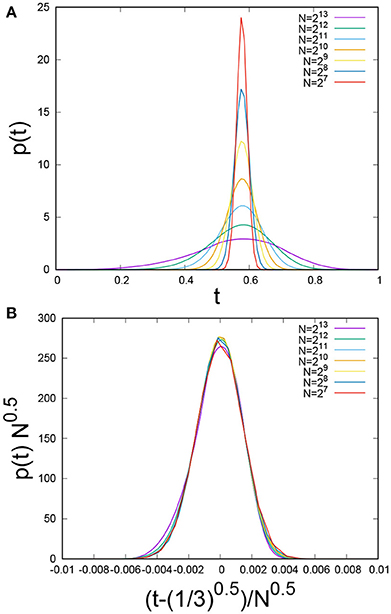
Figure 7. (A) Evolution of the uniform threshold distributions on the unit interval under the real space renormalization group. (B) Rescaling the thresholds leads to a data collapse. The initial number of fibers was N = 2¹⁵. Averages were taken over 10⁶ samples.

which gives $t_c=1/\sqrt{3}$. Since W_N(Δ_N(n), n) is a monotonously increasing function in n, and therefore also Δ_N(n), we must have that t_c is a symmetry point with half the thresholds smaller and half the thresholds larger than t_c. Hence, we have P(t_c) = 1/2. This is what is seen in Figure 6.

We observe numerically that p(t) assumes almost symmetric Gaussian like distribution peaked around the critical load value $t_c=1/\sqrt{3}$. The variance falls off as $1/\sqrt{N}$. We show this in Figure 7 where the data have been fitted to the function

$\begin{array}{rc}p(t)=\frac{1}{\sqrt{N}}\varphi \left(\frac{t-\frac{1}{\sqrt{3}}}{\sqrt{N}}\right);& (47)\end{array}$

where

$\begin{array}{rc}\varphi (y)=Aexp(-B{y}^2),& (48)\end{array}$

with A = 277 and B = 240, 000.

We show in Figure 8 the evolution of the force-load curve under the real space renormalization group, i.e., the equivalent of Figure 4 for the order space renormalization group. For a given cumulative threshold probability P(t), the force-load curve will be given by Equation (19). Hence, the curves seen in Figure 8 reflect this equation combined with Equation (47) giving the evolution of the threshold distribution. Figure 9 shows how the evolution of threshold distribution influences the peak-stress and peak-strain values. After few renormalization steps, peak-stress and peak-strain values converge to same level.

FIGURE 8

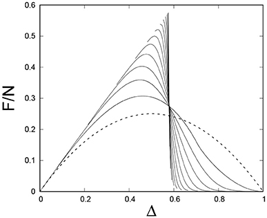
Figure 8. Evolution of the force-load curve under the real space renormalization group. The starting point was 10⁶ fiber bundles each containing N = 2¹⁵ fibers. The threshold distribution was uniform on the unit interval. The dotted curve Δ(1−Δ) is the initial force-load curve.

FIGURE 9

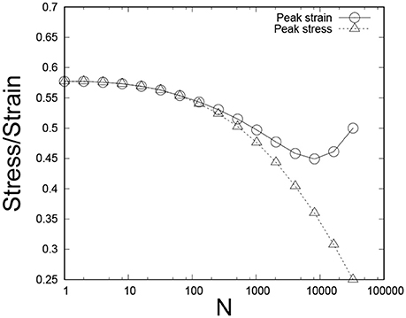
Figure 9. Evolution of the peak-stress and peak-strain under the real space renormalization group. The starting point was 10⁶ fiber bundles each containing N = 2¹⁵ fibers. The threshold distribution was uniform on the unit interval.

The damage parameter d is directly linked to the threshold distribution of the fibers. Under the real space renormalization group scheme, the threshold distribution is not invariant. Hence, d evolves throughout the entire renormalization group iteration and not just toward the end of the process as in the order space renormalization group scheme, see Figure 3. We have shown in Figure 10 the equivalent flow diagram for the real space renormalization group. The flow appears in (Δ, κ, d) space but has been projected into the (κ, d) plane, see Equation (37). There are three fixed points: d = 0, d = d_c and d = 1. The first and the last are stable and d_c is unstable. For the uniform threshold distribution on the unit interval, we have d_c = 1/2.

FIGURE 10

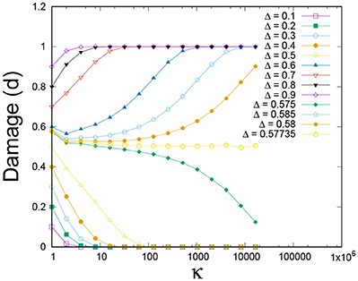
Figure 10. The flow in (Δ, κ, d) space projected into the (κ, d) plane, under the real space renormalization group. Initial number of fibers N = 2¹⁵ having uniform fiber strength distribution on the unit interval. Averages were taken over 10³ samples.

An important aspect of the renormalization group is how fluctuations are handled. Here we consider the avalanche distribution [9, 10, 18]. The size of an avalanche is the number of fibers that fail simultaneously as a result of a change of the external parameters. We consider here a change in the external force F under quasi-static conditions. It was shown under very general conditions that the histogram would follow a power law with exponent −5/2 [18]. We show in Figure 11 the evolution of the avalanche histogram under the real space renormalization group. The power law character of the avalanche distribution remains until the number of fibers in the bundle is too low. The exponent −5/2 remain in place as long as there is a discernable power law.

FIGURE 11

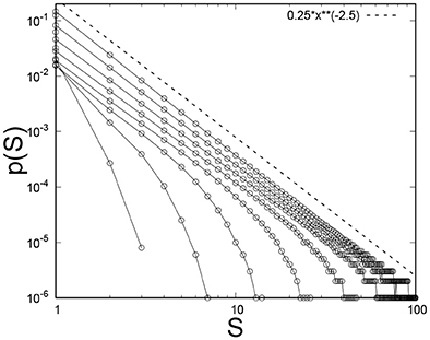
Figure 11. Evolution of the histogram of avalanche sizes as the real space renormalization group is iterated. The initial threshold distribution was uniform on the unit interval. The initial number of fibers was N = 2¹⁴ and averages were taken over 10⁵ samples.

We plot in Figure 12 the average of the largest avalanche occurring before complete failure of the bundle as a function of bundle size N under the real space renormalization group. We see that this average reaches unity—the smallest value it can take on—when the fiber bundle is reduced to a bundle of 2⁵ fibers (we have started with a bundle of 2¹⁴ fibers).

FIGURE 12

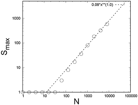
Figure 12. Evolution of the largest avalanche occurring before complete failure as the real space renormalization group is iterated. The initial threshold distribution was uniform on the unit interval. The initial number of fibers was N = 2¹⁴ and averages were taken over 10⁵ samples.

4. Renormalized Strength

Now we are going to compare the initial and final strengths of a fiber bundle, which has gone through the renormalization group scheme. We have, so far only considered the uniform threshold distribution on the unit interval. In the following, we consider a power law on the unit interval,

$\begin{array}{rc}p(t)=(1+\alpha )t^{\alpha },& (49)\end{array}$

where α≥0. When α = 0, we have the uniform distribution. We will study the initial and final fiber bundle strength at imposed load Δ under the order or real space renormalization scheme. The force on a bundle at load Δ is

$\begin{array}{rc}F(\Delta )=N\kappa \Delta (1-P(\Delta ))=N\kappa \Delta (1-{\Delta }^{\alpha +1});.& (50)\end{array}$

By solving dF/dΔ = 0 for Δ gives us the initial strength of the fiber bundle (with N fibers),

$\begin{array}{ll}{({\Delta }_N^c)}_{initial}={(\frac{1}{\alpha +2})}^{\frac{1}{1+\alpha }}.& (51)\end{array}$

Since the work performed on the fiber bundle is conserved by the renormalization group, at the final renormalization step (when N = 1) we must have (see Equation 46)

$\begin{array}{rc}{({\Delta }_N^c)}_{final}^2={\displaystyle \underset{0}{\overset{1}{\int }}}{t}^{2}p(t)dt;& (52)\end{array}$

which gives the final strength of the bundle (with N = 1 fiber)

$\begin{array}{ll}{({\Delta }_N^c)}_{final}=\sqrt{\frac{\alpha +1}{\alpha +3}}.& (53)\end{array}$

Figure 13 compares the initial and final bundle strengths as a function of power law index α.

FIGURE 13

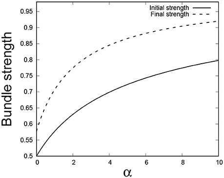
Figure 13. Initial and final strengths of the fiber bundle vs. power law index (α) under both the order space and the real space renormalization group schemes. For α = 0, the distribution is reduced to the uniform distribution and the initial and final strength values match well with our numerical results.

We see that the final strength of a bundle has gone up as a result of the renormalization group scheme ! Our renormalization group transform consists of replacing pair of fibers in the original bundle by single fibers. To keep the energy constant under the trasformation, the strength of the new fiber is chosen according to Equation (33), where the final strength of single fiber is always greater than the average strength of the two initial fibers - and this is the origin of the strength enhancement in the final renormalized strength of the bundle.

5. Conclusion and Discussion

We have in this paper introduced a renormalization group for the equal load sharing fiber bundle model based on formulating the fiber bundle in the context of damage mechanics. The idea behind the damage mechanics formulation is to introduce a continuous damage variable so that the binary nature of the single fibers is no longer in focus. In this way, we are able to group together the fibers belonging to a given fiber bundle into smaller fiber bundles and map the parameters of the larger fiber bundle onto the smaller bundles. A central concept in this mapping is the conservation of the work applied to the fiber bundle to create a certain level of damage, Equation (9). This work is kept invariant under the renormalization group procedure.

We have presented two versions of the renormalization group. In the order space formulation, we group the fibers together according to their failure strength. The three parameters (Δ, κ, d) are mapped according to Equations (23, 24, and 33). Under this version of the renormalization group, the threshold distribution remains invariant (see Figures 1, 2).

The problem with the order space renormalization group scheme is that there is no obvious way to generalize it to other fiber bundle models such as the local load sharing model. Rather than grouping together the fibers according to their strength, we may group them together according to their locations, hence defining the real space renormalization group scheme. The flow Equations are then given by (23, 24, and 45). This real space renormalization groups scheme has been formulated for the equal load sharing fiber bundle model.

In order to formulate a real space renormalization group scheme for fiber bundle models with non-trivial stress redistribution, such as the local load sharing model, it is necessary to replace the equal load sharing model work function W(Δ, d), Equation (9) by one i that takes into account the stress intensification inherent to this model. The coarse graining inherent in the renormalization group equations would then proceed as in the equal load sharing case but with different flow equations ensuing.

We have in this paper only presented the renormalization group schemes themselves together with a number of their properties. We have not attempted to implement the renormalization group on more complex fiber bundle models. We do see a strong potential in the use of the renormalization group as a tool to investigate the fiber bundle models, in particular in connection with fluctuations (see Figure 1) and strength enhancement (see Figure 13).

Author Contributions

SP: Numerical Simulations, data analysis, plotting and some theory; AH: Theory; PR: Theory. Equal contributions in discussions and writing the article.

Conflict of Interest Statement

The authors declare that the research was conducted in the absence of any commercial or financial relationships that could be construed as a potential conflict of interest.

Acknowledgments

The authors thank Martin Hendrick, Jonas T. Kjellstadli and Laurent Ponson for interesting discussions. This work was partly supported by the Research Council of Norway through its Centers of Excellence funding scheme, project number 262644.

References

1. Berendsen HJC. Simulating the Physical World. Cambridge: Cambridge University Press (2007).

Google Scholar

2. Buehler MJ. Atomistic Modeling of Materials Failure. New York, NY: Springer Verlag (2008).

Google Scholar

3. Wilson KG, Kogut J. The renormalization group and the epsilon expansion. Phys Rep. (1974) 12:75.

Google Scholar

4. Fisher, ME Excursions in the Land of Statistical Physics. Singapore: World Scientific (2017).

Google Scholar

5. Bonamy D, Bouchaud E. Failure of heterogeneous materials: a dynamic phase transition? Phys Rep. (2011) 498:1. doi: 10.1016/j.physrep.2010.07.006

CrossRef Full Text | Google Scholar

6. Biswas S, Ray P, Chakrabarti BK. Statistical Physics of Fracture, Breakdown, and Earthquake. Berlin: Wiley-VCH (2015).

Google Scholar

7. Peirce, FT Tensile tests for cotton yarns. “The weakest link” theorems on the strength of long and of composite specimens. J Text Ind. (1926) 17:355.

8. Daniels HE. The statistical theory of the strength of bundles of threads Proc Roy Soc Ser A (1945) 183:243.

Google Scholar

9. Pradhan S, Hansen A, Chakrabarti BK. Failure processes in elastic fiber bundles. Rev Mod Phys. (2010) 82:499. doi: 10.1103/RevModPhys.82.499

CrossRef Full Text | Google Scholar

10. Hansen A, Hemmer PC, Pradhan S. The Fiber Bundle Model. Berlin: Wiley-VCH (2015).

Google Scholar

11. Hu B. Introduction to real-space renormalization-group methods in critical and chaotic phenomena. Phys Rep. (1982) 91:233.

Google Scholar

12. Harlow DG, Phoenix SL. Approximations for the strength distribution and size effects in an idealized lattice model of material breakdown. J Mech Phys. Sols (1991) 39:173.

Google Scholar

13. Batrouni GG, Hansen A, Schmittbuhl J. Heterogeneous interfacial failure between two elastic blocks. Phys Rev E (2002) 65:036126. doi: 10.1103/PhysRevE.65.036126

PubMed Abstract | CrossRef Full Text | Google Scholar

14. Krajcinovic D. Damage Mechanics. Amsterdam: Elsevier (1996).

Google Scholar

15. Abaimov SG. Statistical Physics of Non-Thermal Phase Transitions. Heidelberg: Springer Verlag (2015).

Google Scholar

16. Berthier E. Quasi-Brittle Failure of Heterogeneous Materials: Damage Statistics and Localization, thesis, Université de Paris 6 (2015).

17. Gumbel EJ. Statistics of Extremes. Mineola, NY: Dover(2004).

Google Scholar

18. Hemmer PC, Hansen A. The distribution of simultaneous fiber failures in fiber bundles. J Appl Mech. (1992) 59:909.

Google Scholar