Complex Climate Response to Astronomical Forcing: The Middle-Pleistocene Transition in Glacial Cycles and Changes in Frequency Locking

Through the past few million years large ice sheets have repeatedly grown and disappeared on the Northern hemisphere. These are the Pleistocene glaciations. They are related to the changing solar heating of the Earth due to changes in Earth's orbit and axis of rotation. The climate response to these changes is highly non-trivial and non-linear, expressing the complex nature of the climate system. Many aspects of glacial cycles still need a convincing explanation, one particular mystery being the change from approximately 40 kyr (kilo year) glacial cycles to approximately 100 kyr cycles around 1 million years ago. This transition is called the middle Pleistocene transition (MPT). Here we review some conceptual models to explain the dynamics of glacial cycles and possible dynamical causes of the MPT. We especially focus on the well studied van del Pol oscillator as a conceptual model for the glacial cycles and propose that the MPT is a result of changes in frequency locking of the climate system to the astronomical forcing. This is compared to a recently presented model that relates the MPT to a transcritical bifurcation in the structure of a generic critical/slow manifold for a fast-slow dynamical system.

1. Introduction

The climate of the planet is governed by the radiative energy balance between heating by short wave radiation from the Sun and cooling by the long wave radiation back to space. The heating changes with latitude, thus “climate” is derived from the phrase “inclination,” alluding to the position of the Sun in the sky. The geographic temperature variations result from the transport of heat poleward by winds and ocean currents. These fluid motions are in turn governed by the differential heating via buoyancy and the planetary rotation. Many internal dynamical factors play a role in determining the climate: for example, the amount of snow and ice influences the fraction of sunlight being reflected back into space without heating the planet, the interchange of CO₂ between ocean and atmosphere influences the greenhouse trapping of heat in the atmosphere and the Atlantic overturning circulation influences the oceanic heat transport to the polar regions. The strength of these factors depends in turn on the state of the system, thus constituting non-linear feedbacks for determining the equilibrium state.

State-of-the-art numerical climate models are based on integrating the fluid equations of the atmosphere and oceans and calculating the radiative balance and interactions between atmosphere, oceans, cryosphere (ice masses), lithosphere (soils) and biosphere (vegetation). These “Earth System Models” arguably do a good job in reproducing the present state of the climate, but they are so huge and computationally demanding that it is unclear to what extend the full range of natural variability is represented in the existing models [1]. The most spectacular manifestation of natural climate variability is the glacial cycles, which, since their discovery in the nineteenth century, have been considered a major challenge in climate modeling and theory. With the present day focus on global warming, it is perhaps not fully appreciated that this is still a major challenge.

Large land ice sheets appeared in the northern hemisphere around 3 Ma BP (million years before present). These ice sheets have been waxing and waning with astronomical changes to incoming solar radiation (insolation). The climatic response to the astronomical forcing is, however, far from linear and depends on internal dynamics and feedback mechanisms. Several climate components have been proposed to influence the glacial cycles. These include asymmetric ice sheet response to insolation in buildup and collapse phases [2] and positive ice-albedo feedback [3, 4] (more ice gives more reflection leading to less heating, thus lower temperature, and hence more ice). The dominant factor could be ice sheets [5] or sea ice [6]. It could also be an interplay between ice volume, greenhouse gas warming, and interchange of CO₂ between the atmosphere and oceans depending on ocean temperature [7], or coupling between greenhouse gas concentration, ice volume and areal extend of the Antarctic ice sheet [8].

In terms of the climate response to astronomical forcing, the proposed models of glacial cycles vary between emphasizing the dominance of internal stochastic variations [9], scaling properties of climate variations [10, 11] and stochastic resonance [12] to self-sustained non-linear oscillations [13] and forced non-linear oscillations [14]. A comprehensive review of existing models of ice ages is discussed in Crucifix [15] and we refer the reader there for more details.

Here we shall focus on possible mechanisms for the climate response to astronomical forcing assuming the climate system to have internal dynamical oscillations. The astronomical forcing is the change in seasonal and geographically distributed amount of insolation. These variations are due to perturbation of Earth's orbit from the other planets, and is dominated by only three parameters; the precession of Earth's axis of rotation, the obliquity, which is the variation in the tilt of the axis of rotation with respect to the orbit and lastly, the change in the eccentricity in the orbit. The periodicities of these variations are approximately 20-, 41-, and 100 kyr respectively. The frequencies are incommensurate, so the forcing is quasi-periodic. The annually integrated insolation is dominated by the ~ 41 kyr obliquity cycle. We will thus not be concerned with the quasi-periodic nature of the forcing. Our focus is on possible mechanisms for synchronization of the climate response to the dominant periodic obliquity cycle, especially how the MPT can be explained. As mentioned above, several oscillator models have been proposed for the glacial cycles, here we chose the well studied van der Pol oscillator as a generic example. We also consider a somewhat more complex, recently proposed by us [16] as an embedding of a switching model of Paillard [17]. For the latter model, the MPT involves a transcritical bifurcation in the structure of a generic critical/slow manifold for a fast-slow dynamical system. In order for this paper to be self-contained for non-expert readers, we also review a few theoretical aspects.

2. The Last Glacial Period

The climate history in proxy records (notably isotope ratios in sediment and ice cores) shows violent shifts between different global temperature states, which seem not to be well captured in most models. Sudden climate changes can occur if the system reaches a threshold, a tipping point, where the internal feedbacks lead to the climate irreversibly making a transition from one state to another. These paleoclimatic records indicate that the transition from the last glacial to the present warm interglacial occurred as such a threshold crossing [18]. By comparing the insolation with the temperature proxy obtained from a Greenland ice core through the past 60 kyr (kilo years) it is apparent that the relation between the insolation (forcing) and the temperature (response) is not linear, see Figure 1. The temperature changes are much more abrupt than the changes in insolation, and the response seems to be much more dramatic than the change in the forcing would suggest. The insolation curve has been scaled and shifted in order to linearly fit the climatic response in the present Holocene climate (10 kyr BP to present). The fit clearly breaks down for the glacial period. For this period the insolation curve needs to be shifted downward with an amount that is almost a factor three larger than the variation over time (blue curve). This strongly suggests that the climate system jumps non-linearly from one equilibrium state to another, and within such an equilibrium state the response to the changing insolation is linear. Furthermore, the glacial climate is characterized by a splitting into the stadial (cold state) and the interstadial (intermediate) state. These jumps are the Dansgaard-Oschger climate events [19]. The quasi-equilibrium or mean state within each of the three climate states seems to be linearly related to the insolation (green curve).

FIGURE 1

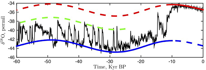
Figure 1. The NGRIP isotope record [18] for the past 60 kyr is a proxy for temperature. The red, green and blue curves are the summer insolation at 65N fitted to the climate record. The red curve is fitted to the present Holocene climate, the blue curve is shifted to fit the cold stadial state, while the green curve is shifted to fit the interstadial states.

3. Multiple Climate States

Considering the global energy balance of the Earth, a minimal climate model can be constructed. This was done independently by Budyko [3] and Sellers [4]. The essence of the Budyko-Sellers energy balance model is considering the surface temperature as represented by a single (average) temperature, T. The temperature is governed by the balance between the total incoming solar radiation, R_i, and the total outgoing gray-body radiation, R_o: namely cṪ = R_i − R_o, where c is the heat capacity of the atmosphere and upper part of the oceans, which is in thermal contact with the atmosphere. Part of the incoming radiation from the Sun will be reflected back into space, thus not contributing to the heating. The reflected part is governed by the planetary albedo, α(T), which in turn depends on temperature through the amount of reflecting ice area. This positive feedback is balanced by the negative black body feedback: lower temperatures give less outgoing black body radiation which in turn decelerates the temperature drop. The energy balance equation is:

$\begin{array}{ll}cṪ=(1-\alpha (T))S-g(T)\sigma T^4,& (1)\end{array}$

where S is the solar constant, or rather the integrated insolation, g(T) is the grayness factor of the planet, accounting for the greenhouse effect of the atmosphere and σ is the Stefan-Boltzmann constant.

In order to proceed, the functions α(T) and g(T) must be specified. The planetary albedo can in the simplest way be modeled as a sigmoidal function of temperature, observing the asymptotic limits; for high temperatures the albedo is that of the hot ice free planet, α_H, while for low temperature the albedo is that for the cold completely ice covered white planet, α_C. We model this using α(T) = (α_H + α_C)/2 + (α_H − α_C)arctan((T − T₀)/Σ)/2. The grayness factor can also be modeled in different ways. An instructive way is to account for the (natural) greenhouse warming ΔT, by noting that the long wave opacity of the atmosphere implies that the black body radiation from the planet is governed by an effective radiation temperature at the infrared optical depth from above of the atmosphere, T_eff = T − ΔT, $R_o=\sigma T_{\text{eff}}^4$, thus expressed in terms of surface temperature, we obtain g(T) = (1 − ΔT/T)⁴. We may define a “climate potential” $U(T)=\stackrel{T}{\int }\left[R_i(S)-R_o(S)\right]dS$, in order to bring the model to the familiar form:

$\begin{array}{l}cṪ=-dU/dT.\end{array}$

This is a very simple model of the global energy balance, illustrating the principles in multiple steady climate states. With the insolation defined as S_μ(t) = S + μ(t), and a large enough harmonic variation of the parameter μ₀: μ(t) = μ₀cosωt, the system will respond through the classical hysteresis loop (Figure 3, top panel).

However, this is not a realistic model of glacial cycles for two reasons. Firstly, the astronomical change in insolation through a glacial cycle is not large enough to bring the climate through the hysteresis loop of consecutive bifurcations between the cold and the warm climates. This problem was the original inspiration for the model of stochastic resonance [12]. Assuming that the amplitude of the varying forcing is not large enough to cross the bifurcation point, the transition could be assisted by noise,

$\begin{array}{ll}cṪ=-dU/dT+\sigma \eta ,& (2)\end{array}$

where η is a unit variance white noise (more precisely, we consider the Itô SDE $cdT=-U^{\prime }(T)dt+\sigma d{W}_t$ where W_t is a standard Wiener process). If the noise intensity σ is small then the noise will only rarely trigger transitions, if the noise intensity is high then the noise will trigger frequent transitions regardless the periodic change of the forcing. If the noise intensity is such that the mean stochastic escape time is comparable to half a forcing period, it will trigger transitions in conjunction with the forcing at the times when the system is close to the bifurcation. At this noise intensity the periodicity of the forcing is restored in the response, thus the term stochastic resonance [12]. By considering the double-well potential in Figure 2, middle panel, the resonance can be understood in terms of time scales: The escape time from the deep well (a) to the shallow well (c) is ${\tau }_{a\to c}~exp\left[(U_b-U_a)/{\sigma }^2\right]$, where U_b is the potential at the barrier, thus U_b − U_a is the height of the barrier from the left well, the other way is ${\tau }_{c\to a}~exp\left[(U_b-U_c)/{\sigma }^2\right]$. The periodic forcing, with period T = 2π/ω, will cause the deep and shallow wells to change positions, disregarding unimportant asymmetries, so if τ_{c → a} ≪ T ≪ τ_{a → c}, the noise will cause the system to move periodically between the two states. This is shown in Figure 3, middle panel. The extreme case of no forcing and solely noise induced transitions is shown in the bottom panel. This resembles the interstadial states observed in the glacial period in the ice core record (Figure 1).

FIGURE 2

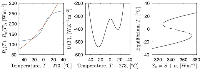
Figure 2. The global energy balance model. The left panel shows incoming radiation, R_i(T), in blue and the outgoing radiation R_o(T) in red. There are three steady state points; two stable separated by an unstable. The middle panel shows the equivalent “climate potential" as a double well potential. The right panel shows the bifurcation diagram obtained by changing the insolation S_μ = S + μ. The stable cold and warm states (solid lines) are connected at two saddle-node bifurcations via an unstable steady state branch (dashed line).

FIGURE 3

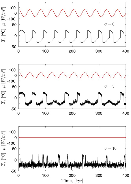
Figure 3. The non-linear response of the energy balance model for the climate (1) to harmonic variations in the insolation: μ(t) = μ₀cosωt when μ₀ is large enough for crossing the two bifurcation points.(top panel). With a noise component with intensity σ (2) added, the response is at the frequency of the forcing, even though the forcing itself does not cause crossing of the bifurcation points. This is called stochastic resonance (middle panel). If the noise intensity is large enough, even without periodic forcing, the system will jump stochastically as a Poisson process with little sign of periodicity. This is termed noise induced transitions (bottom panel).

The second, and more important, reason why this is not a realistic model is that the glacial climate state does not correspond to a state of global ice cover, such that the planetary albedo becomes insensitive to further cooling. However, though the model was proposed as a model of glacial cycles, it turned out to have even bigger merits: Very few predictions have been obtained from climate theory, but considering the present climate as the warm state, the model predicts a deep freeze climate state. Such a state has now been identified, namely the Snowball Earth, which occurred at least twice approximately 700 Myr ago [20].

4. Glacial Cycles and the Change in Response to Astronomical Forcing

Returning to glacial cycles earlier than the last glaciation, the ice volume is recorded as a proxy in oxygen isotopic composition of benthic foraminifera in ocean floor sediments. The concentration of heavy water in the ocean increases when the ice sheets on the continents grow. This is due to the isotopic fractionation in evaporation and condensation, such that water falling as snow on land is depleted from heavy isotopes. Thus the sediment record is a direct proxy for the global ice volume, which in turn is related to the temperature. Extending the insolation curve, red curve in Figure 1, over two million years and comparing it with the proxy temperature record, it is clear that the relation is far from being simple linear (Figure 4). The insolation is a composite of three astronomical many-body perturbations to the Keplerian orbit: The eccentricity of the orbit changes with periods around 100 kyr, the inclination of Earth's axis of rotation with respect to the Ecliptic plane, the obliquity, changes with a period of 41 kyr and finally the precession of Earth's axis, determining the seasonal distance to the Sun in the elliptic orbit, has a period of approximately 20 kyr. The red curve in Figure 4. represents the annually integrated insolation at 65N. This is the approximate latitude of the southern rim of the glacial time ice sheets. The insolation at this latitude is thus the forcing proposed to govern the waxing and waning of the ice sheets [21]. This integrated insolation curve is dominated by the 41 kyr obliquity cycle [22].

FIGURE 4

Figure 4. The global stacked sediment isotope record from benthic foraminifera (black) along with the 65N insolation curve (red, arbitrary units) from Figure 1. The gray lines show how each interglacial warm maximum is related to the nearest maximum of the insolation curve. The isotope record is a proxy for global ice volume and thus temperature. Note that the scale is inverted, such that temperature increases along the y-axis. The ice-core record in Figure 1 corresponds to the very last glacial cycle. The ocean record does not resolve the fast stadial-interstadial oscillations. In order to quantify the visual association a spectral analysis is shown in the lower part. The contour plot shows the power spectrum of the record in a 400 kyr running window (indicated by the black bar). The center point of the window is on the x-axis, while the frequency is on the y-axis. The upper contour corresponds to approximately 1/40 kyr⁻¹, present in the full record. The lower contour corresponds to approximately 1/100 kyr⁻¹ only being predominant after the MPT.

The approximate 100 kyr eccentricity cycle is barely visible in the astronomical forcing curve [21], while the climate record shows glacial cycles of approximately 100 kyr for the past million years. Before that time the glacial cycles had a smaller amplitude and a period close to the 41 kyr obliquity cycle. The transition from the “40 kyr world” (or rather “41 kyr world”) to the “100 kyr world” is termed the middle Pleistocene transition (MPT). For visualization, each interglacial warm maximum is related to the nearest maximum in the insolation curve (gray lines in Figure 4). The dating uncertainty in the sediment record is such that these can be considered synchronous [23]. A spectral analysis, where the power spectrum is calculated for a running 400 kyr window is shown in the lower part of Figure 4. It shows that the 40 kyr oscillation persists through the record, while the spectral power around 100 kyr increases from around 1.2 Myr BP to a strong power after 800 kyr BP. Thus the MPT can be seen as a gradual change of glacial duration in the period 1200 - 800 kyr BP [24]. Another way of interpreting the change at the MPT is that the duration of the glacial periods increases and the interglacials synchronize to every second insolation maximum from around 1 Myr and every third insolation cycle from around 500 kyr. This complex climate response to astronomical forcing indicates that the glacial cycles could be explained as a non-linear frequency locking phenomenon.

5. Conceptual Models for Glacial Cycles

Though glacial cycles may eventually be reproduced in the large Earth system model simulations, this is not feasible with present day computers. The Earth system models do in some sense correspond to calculating the behavior of many-body systems from first principles. However, a satisfactory theory of ice age dynamics should involve some reduction of the complexity of the full set of governing equations. The regularity of the paleoclimatic record, and the low-dimensionality in the astronomical forcing make it plausible that the dynamics of a low number of leading modes can be captured by a few effective dynamical equations. The fundamental conjecture in the following is that the system has inertia in the sense that the regulating feedbacks can lead to internal oscillatory behavior. Whether this is the case is unknown, but several factors in the climate system could play the role of such an inertia: The simplest heuristic climate oscillator is obtained by considering the continental ice volume x. Its growth is proportional to the precipitation p [25]:

$\begin{array}{l}ẋ~p.\end{array}$

The precipitation increase with temperature,

$\begin{array}{l}p~T,\end{array}$

but the temperature decrease with the ice volume, due to the ice albedo feedback,

$\begin{array}{l}\alpha ~x,\end{array}$

and from the energy balance (1) we get;

$\begin{array}{l}Ṫ~-\alpha ~-x.\end{array}$

Substituting for T and p, we obtain

$\begin{array}{l}ẍ~-x,\end{array}$

as a schematic climate oscillator.

The climate variable of interest and observed in the sediment record, is the global continental ice volume x. The waxing and waning of the ice sheets are governed by the mass balance between accumulation, proportional to the precipitation, and the ablation or melt-off. Both terms depend on the atmospheric temperature. With the anomaly y~ (accumulation − ablation), we get

$\begin{array}{l}ẋ=y.\end{array}$

The temperature, and in turn y, depends through ice-albedo feedback, changing atmosphere - and ocean circulation, ocean-atmosphere exchange of CO₂ etc. on the ice volume x itself; ẏ~ − αx, where we may just think this as the first term in a Taylor expansion of the complicated non-linear dependence on x.

The internal stabilizing dynamics of the anomaly y can be described as a Newtonian cooling or dissipation: g(x)y, where the rate g(x) can depend on the ice volume x. Finally y depends on the astronomical insolation anomaly F(t):

$\begin{array}{l}ẏ=-g(x)ẋ-\alpha x+F(t).\end{array}$

We shall not attempt to argue for the physical realism of the conceptual model, but focus on the dynamical effects of the response to the astronomical forcing. The reason for choosing this specific form for the model is that by substituting for ẏ, and choosing g(x) = −γ(1 − x²), this becomes the well studied forced van der Pol equation [26] for the variable x:

$\begin{array}{ll}ẍ=\gamma (1-x^2)ẋ-\alpha x+F(t),& (3)\end{array}$

The astronomical forcing is assumed to be a pure harmonic: F(t) = Acos(ω_Ft), where ω_F = (2π/41) kyr⁻¹ corresponding to the main obliquity cycle. Thus the multi-frequency, quasi-periodic nature of the orbital forcing [27] is not the concern here. The van der Pol equation has a surprisingly complex behavior depending on the specific values of the parameters of the model. We may reformulate the equation in terms of motion subject to a conservative force −dU/dx, where the potential is given by $U(x)=\frac{1}{2}\alpha x^2$.

The non-linearity enters through the dissipation term, which can act both as a damping (for x² < 1) and as a forcing (for x² > 1).

5.1. The Linear Damped and Forced Harmonic Oscillator

The trivial case g(x) = γ is just the simple linear damped and forced harmonic oscillator: The linear oscillator is not a very realistic model of ice age cycles, but it can capture some aspects of internal ice sheet dynamics [13]. The periodically forced damped harmonic oscillator ($\alpha ={\omega }_0^2$):

$\begin{array}{ll}ẍ=-\gamma ẋ-{\omega }_0^{2}x+Acos{\omega }_{F}t& (4)\end{array}$

will always oscillate with the forcing frequency ω_F and an amplitude given by the resonance curve:

$\begin{array}{l}{A}_0=A/\sqrt{{({\omega }_0^2-{\omega }_F^2)}^2+{\omega }_F^2{\gamma }^2}.\end{array}$

The response has maximum amplitude at the resonance frequency ω₀ = ω_F. (Note that this is slightly different from the textbook example of tuning ω_F to the resonance with fixed ω₀ and γ, where we get ${\omega }_F=\sqrt{{\omega }_0^2+{\gamma }^2/2}$). Only the transient solution will have a natural frequency ${\omega }_t=\sqrt{{\omega }_0^2+{\gamma }^2/4}\approx {\omega }_0$. The oscillator will, after the transient has died out, always be in a 1:1 frequency relation to the forcing with an amplitude and phase depending on the difference between the natural frequency and the forcing frequency. The damping implies that the unforced oscillator will die out, x = ẋ = 0 being a stable fixed point. There are thus no self-sustained oscillations. In the Hamiltonian case of no damping and forcing, the system will oscillate with a periodic orbit in phase space depending on the (conserved) energy $2E={(A_0{\omega }_0)}^2={ẋ}^2+{\omega }_0^2{x}^2$. There are thus no isolated orbits (limit cycles) in the Hamiltonian case. In the damped and forced case x(t) = A₀cos(ω_Ft + θ) is the globally attracting (stable) limit cycle.

The situation is different for the (non-linear) van der Pol oscillator as we will see.

5.2. The Glacial Cycles as a Self-Sustained Oscillation Synchronized to Astronomical Forcing

Consider the forced van der Pol oscillator as a model of the glacial cycles. This was proposed as a minimal model [15, 27], with the distinct advantage of having well-understood dynamics [26, 28].

In contrast to the damped linear oscillator, the van der Pol oscillator has oscillations even in the autonomous unforced case (A = 0). The dissipation term g(x) = −γ(1 − x²) grows the oscillations when x² < 1 and damps the oscillations when x² > 1. For γ ≫ 1, the van der Pol oscillator is a fast-slow system that has relaxation oscillations: the stress accumulated during a slow build up is relaxed during a fast discharge. This can be seen by applying the Liénard transformation y ≡ x − x³/3 − ẋ/γ to (3). By a straightforward substitution [28], we get:

$\begin{array}{l}ϵx^{\prime }=x-x^3/3-y\end{array}$

$\begin{array}{ll}{y}^{\prime }=\alpha x-Acos{\omega }_{F}t,& (5)\end{array}$

where ϵ = 1/γ² and the time derivatives are with respect to a slow time τ = t/γ. It is apparent that γ ≫ 1 defines a slowly forced fast/slow (x/y) system for ϵ → 0. A good sense of the behavior of the unforced system, A = 0, is obtained by observing the nullclines ẋ = 0⇒y = x − x³/3 and ẏ = 0⇒x = 0, see Figure 5. The fixed point (x, y) = (0, 0) is an unstable focus (for γ > 0). The oscillator has a stable limit cycle, a slow-fast system, with two slow branches (the critical/slow manifold: ẋ = 0) connected by two fast branches. The existence of the limit cycle in the unforced case implies that the van der Pol oscillator has an internal natural frequency ω₀ = 2π/T₀, where T₀ is the period of the cycle.

FIGURE 5

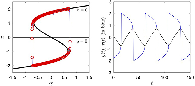
Figure 5. The van der Pol oscillator (5): The left panel shows the phase plane. The black curves are the nullclines. A trajectory is shown in blue. The dots marking the trajectory at equal time intervals indicate two slow branches near the x-nullcline. The right panel shows that this is a slow/fast dynamical system with the fast variable x(t) (in blue) closely following the x-nullclines (critical/slow manifold) interrupted by fast jumps from one branch to the other. The slow variable y does not change at the jumps. Parameters are (α, γ)=(1, 5).

In the forced case (3), the oscillator frequency can synchronize to the forcing frequency in a rational relation between the oscillator frequency ω and the forcing frequency ω_F depending on the amplitude of the forcing A and on the ratio of the two frequencies. Note that there are now three frequencies at play; ω₀ = ω₀(α, γ) is the frequency of the unforced oscillator for a given set of parameters, ω_F is the (constant) forcing frequency and finally ω = ω(α, γ, A, ω_F) is the frequency of the forced oscillator for a given set of parameters, assuming that the oscillator has a limit cycle.

The periodicity of the response can be identified in a stroboscopic map, a special case of a Poincaré map were the Poincaré section is defined by the period of the forcing: x_n = x(t_n), t_n = nT_F + t₀ with T_F = 2π/ω_F being the period of the forcing. The number of limit points of the set ${\left\{x_n\right\}}_{n=1}^{\infty }$ is the periodicity of the system in units of the forcing period. The stroboscopic map {x_n} and ω₀ will depend on the parameters (α, γ, A, ω_F). In Figure 6 the trajectory sampled as a stroboscopic map {x_n} is shown as a function of ω₀(α, γ)/ω_F, corresponding to increasing the parameter α with fixed values of γ and A. For ω₀/ω_F > 1.35, we observe a single branch, thus ω = ω_F while for 1.03 < ω₀/ω_F < 1.09 we observe two branches, thus ω = ω_F/2 (i.e., the period is T = 2T_F), for ω₀/ω_F < 0.98 we obtain three branches, thus ω = ω_F/3. In the three cases the system synchronizes to the forcing in ratios 1:1, 2:1 and 3:1 respectively. Between these locking regions there is stable quasiperiodic motion intersected by windows with higher rational ratios of synchronization.

FIGURE 6

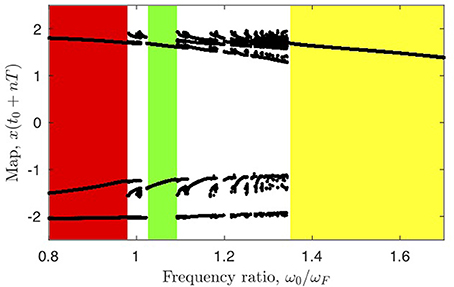
Figure 6. Bifurcation diagram showing the stroboscopic map for the van der Pol oscillator (3) as a function of the ratio of the unforced internal frequency to the forcing frequency, ω₀/ω_F, obtained by varying parameter α with A = 0.2 and γ = 5 fixed. The colored regions corresponds to synchronization: 1:1 (yellow), 2:1 (green) and 3:1 (red). Regions with disconnected dots correspond to higher rational synchronization or quasiperiodic motions.

In Figure 7, the synchronization is shown in a color coded plot of the period of the van der Pol oscillator as a function of ω₀/ω_F and the amplitude A of the forcing. For each value of (α, A) in a fine grid, we solved (3) numerically and measured the period of the limit cycle in units of the forcing period T_F. A pattern of tongues in the corresponding parameter (ω₀/ω_f, A) plane is found. In each uniformly colored tongue (called mode-locking regions or Arnold tongues [29]), the oscillator synchronizes onto the external periodic forcing. In the unlocked regions (white areas), no periodic solutions are found. In this case, the ratios between the internal frequency of the system and the driving frequency passes through irrational values (quasi-periodic motion).

FIGURE 7

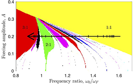
Figure 7. The response of the van der Pol oscillator (3) as a function of the forcing amplitude A and the parameter α. The oscillator frequency ω synchronizes in rational ratio to the forcing frequency ω_F. The colored patches of synchronization are called Arnold tongues. The ordinate is ω₀(α)/ω_F, obtained by calculating ω₀ for A = 0 as a function of α. The parameter γ is kept fixed at γ = 5. The arrow with time ticks indicates the change corresponding to the change of α through the MPT shown in Figure 8.

If the glacial cycles are modeled by this forced oscillator, the MPT could be caused by a slow drift of the internal parameter α, which would change the synchronization to the external astronomical forcing by bringing the system from a 1:1 tongue through a 2:1 tongue to a 3:1 tongue as indicated by the arrow in Figure 7. This scenario is shown in Figure 8. This climate curve is quite robust with respect to how the slow change of the parameter α happens around the MPT. For such a simple conceptual model we cannot expect to associate α with a single slowly changing physical parameter in the climate system. However, suggestions have been that the ocean-atmosphere concentration of CO₂ has been slowly decreasing [30], with reduced greenhouse warming making larger ice sheets sustainable. However, the atmospheric CO₂ concentration at the MPT is not well constrained, and a gradual decrease in CO₂ has been questioned [31]. Another suggestion is that ice sheet stability depends on bottom sliding, such that long term regolith erosion by the North American ice sheets let to the possibility of larger stable ice sheets resting on bedrock after the MPT [32].

FIGURE 8

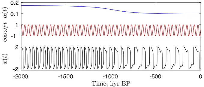
Figure 8. By a slow change of the parameter α(t) the van der Pol oscillator (3) moves from a 1:1 synchronization tongue via a 2:1 to a 3:1 synchronization. The time scale is adjusted to the paleoclimatic time scale in Figure 4. The forcing frequency is 41 kyr corresponding to the obliquity cycle.

6. Bifurcations and the MPT

In addition to the slow drift through synchronization regimes discussed in the previous section, several other conceptual models have been proposed for the glacial cycles in general the MPT in particular. We refer to Crucifix [15] for a more comprehensive review. Here we discuss two different proposals for modeling the MPT in terms of bifurcations. The first of these is a classical low dimensional model proposed for the glacial cycles and the MPT as a Hopf bifurcation by Maasch and Saltzman [33]. The second of these is an alternative model that involves a bifurcation in the topology of the slow manifold [16].

6.1. The MPT as a Hopf Bifurcation

The model by Maasch and Saltzman [33] (in anomaly variables) is a set of three coupled ODEs:

$\begin{array}{l}ẋ=-x-y-I(t)\\ ẏ=-px+ry+s{z}^2-y{z}^2\\ ż=-q(x+z)& (6)\end{array}$

Here x represents the global ice volume, y represents the atmospheric CO₂ (greenhouse gas) concentration and z represents a deep ocean temperature. All variables are rescaled to dimensionless form, p, q, r, s are parameters, while I(t) = Acosω_Ft represents the astronomical forcing (insolation). Heuristic arguments for the physical basis of the model are given in [33]. These concentrate on the greenhouse effect, temperature dependent interchange of CO₂ between oceans and atmosphere and the dependence of ice volume on the atmosphere. The model has a rich structure in parameter space Maasch and Saltzman [34]. By design, there is a fixed point of the autonomous model (I(t) = 0) at x = y = z = 0 for all parameter values, while for s² > 4(p − r) there are two more non-trivial fixed points. Concentrating on the fixed point (0, 0, 0), linear stability shows that this is stable for small values of the parameter r (keeping all other parameters fixed) and becomes unstable for some critical value, r > r_c, through a simple Hopf bifurcation.

The hypothesis in this model is that the MPT is this Hopf bifurcation: Prior to the MPT the system is oscillating around the stable fixed point with the external oscillation I(t) = Acosω_Ft, after the Hopf bifurcation the 100 kyr glacial oscillations are the internal oscillations. This is seen in the forced realization of the model in the lower black curve in Figure 9. The top blue curve shows a slow increase of the parameter r through the MPT, similar to the change of the parameter α in Figure 8. With this choice of parameters the bifurcation point is crossed around the MPT, but the amplitude of the internal oscillations grows very slowly in the autonomous case (A = 0).

FIGURE 9

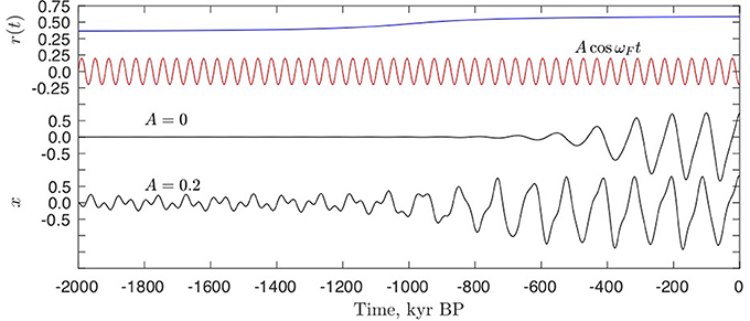
Figure 9. By a slow change of the parameter r (top blue curve) the system (6) passes through a Hopf bifurcation. The other parameters are fixed: (p, q, s) = (1.0, 1.2, 0.8). The two lower black curves are the x variable in the autonomous case (A = 0) and in the forced case (A = 0.2). The autonomous system reaches the Hopf bifurcation for r = 0.35. The red curve is the forcing.

In the non-autonomous case (A = 0.2) the oscillations of the forcing can be seen as a linear response in the climate variable x prior to the Hopf bifurcation. After the bifurcation the internal 100 kyr oscillation dominates independently from the forcing. However, prior to the bifurcation where the fixed point is stable, if the system is perturbed away from the fixed point by an additional small stochastic forcing the system will respond with decaying oscillations with the internal period of the limit cycle after the Hopf bifurcation see Figure 10. Thus the external forcing period is not robustly imprinted on the climatic response prior to the MPT. As a dissipative non-linear oscillator with parameter dependent internal frequency after the Hopf bifurcation, a scenario of synchronization analogous to that of the van der Pol oscillator is possible.

FIGURE 10

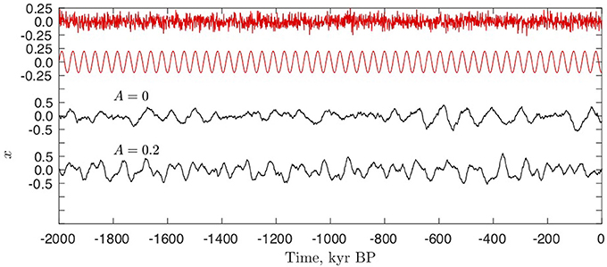
Figure 10. Same as Figure 9, but now keeping the parameter r = 0.25 constant at a value prior to the Hopf bifurcation, where the fixed point is stable. In this case stochastic terms ση_x, ση_y and ση_z are added to the right hand side of (6), η_{x, y, z} are unit variance Gaussian white noise and σ = 0.08, a corresponding noise curve is shown for illustration, (top red curve). This is on same time scale as the astronomical forcing with A = 0.2. Even with astronomical forcing, the internal 100 kyr oscillation dominates the climate signal x.

6.2. The MPT as a Bifurcation of the Slow Manifold

As the global energy balance model shows, the climate system can be in one of a number of stable states under identical external conditions. By a change of a control parameter, in this case the insolation, the system can cross a saddle-node bifurcation point, and jump from one stable branch to the other. This is typical hysteresis behavior, similar to relaxation oscillation between the two slow branches of the van der Pol oscillator. The scenario could describe the glacial cycles prior to the MPT. After the MPT the amplitude of the oscillation between the warm and the cold state increases (Figure 4), in contrast to what is observed in the van der Pol scenario above. Furthermore, the oscillations seem to become more time asymmetric with rapid warming and gradual cooling through the cold climate state experienced prior to the MPT and to an even colder state with more extended land ice cover.

From these observations an empirical model was proposed by Paillard [17]. Assume that the glacial cycles prior to the MPT was an oscillation between two stable states or branches i, interglacial, and g, a mild glacial state: i → g → i. At the MPT a third deep glacial state G became “accessible.” The 100 kyr glacial cycles thus involve a series of transitions: i → g → G → i. The time asymmetry thus reflects the difference between the gradual inception (entering the glacial state) i → g → G and the abrupt termination (of the glacial state) G → i. This dynamical behavior, where transitions i → G and G → g are “forbidden” is generically described through a sequence of bifurcations with a generalized hysteresis behavior [35]. In order to describe the scenario a model was proposed [16] where the slow dynamics of the ice volume v(t), as observed in the paleoclimatic record is coupled to a fast unobserved temperature variable x(t), through an effective set of coupled ordinary differential equations (ODEs):

$\begin{array}{l}\dot{v}=G(x,v)-I(t)\end{array}$

$\begin{array}{ll}ẋ=H(x,v,\lambda ).& (7)\end{array}$

The term I(t) represents the time dependent astronomical forcing (insolation), where the minus reflects that the ice volume shrinks with higher insolation. The parameter λ(t) represents some independent slowly varying forcing which changes the structure of the critical/slow manifold, i.e., of the zero set of H(x, v, λ).

In the autonomous case (I(t) = I₀ and λ(t) = λ₀) the (2D) dynamics is limited to stable or unstable fixed points, limit cycles or homoclinic (heteroclinic) orbits connecting fixed point(s). As with the van der Pol oscillator we shall assume this to be a fast-slow system, with the dynamics of the climate variable x being much faster than the dynamics of the global ice volume v; τ_x≪τ_v. The dynamics will thus be close to the stable branches of the critical/slow manifold determined by ẋ = H(x(v, λ), v, λ₀) = 0. This is similar to the dynamics of the van der Pol oscillator, where the critical/slow manifold is the x-nullcline (Figure 5). The dynamics of v can be chosen to be a simple slow relaxation to an equilibrium volume v_e(x) depending on the fast temperature variable x:

$\begin{array}{ll}G(x,v)=-(v-v_e(x))/{\tau }_v(x)& (8)\end{array}$

The equilibrium volume v_e(x) is a linearly decreasing function of temperature, the large relaxation time scale τ_v(x) is likewise a decreasing function of x, reflecting that in the cold glacial climate both melting and accumulation are small giving a slower adjustment to equilibrium. For more details see [16] and the Appendix.

6.3. Geometry of the Bifurcation on the Slow Manifold

The x-nullcline, or critical manifold, is determined by the surface H(x(v, λ), v, λ) = 0 in the (x, v, λ) space. Now, since the function H(x, v, λ) is determined empirically from the observed climate record, i.e., not at the present level determined from first principles, the bifurcation structure must be as generic as possible given the observations. This means that it must be constructed with a structure that is robust with respect to small perturbations. In 1 dimension the only generic bifurcation is the saddle node, while in 2 dimensions cusp and Hopf bifurcations are generic [36]. Moreover, if we consider the bifurcations of the critical manifold on varying a parameter λ independent of both fast and slow dynamics, two saddle nodes may generically meet at a transcritical bifurcation.

We postulate that prior to the MPT, for a fixed value of λ(=0.1), the x-nullclines are as shown in the left panel in Figure 11. At the MPT, as λ changes, the system goes through a transcritical bifurcation (middle panel). After the MPT the x-nullclines are as in Figure 11, right panel. In all cases the stable branches are shown in black, while the unstable branches are shown in gray. Figure 12 shows the dynamics (7) for I(t) = Acosω_Ft, where the transcritical bifurcation is crossed for λ = 0. Sections of the trajectory around the corresponding value of λ are shown in Figure 11 left and right panels. This fast-slow dynamics is analogous to the van der Pol oscillator (Figure 5).

FIGURE 11

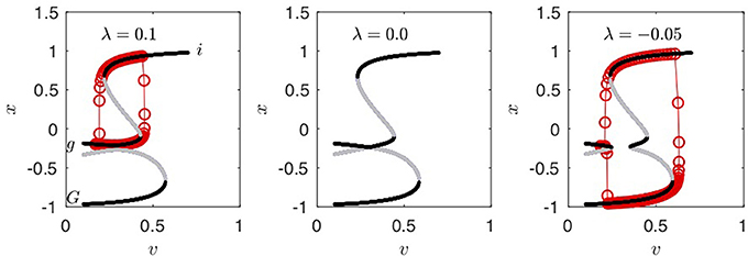
Figure 11. The parameter λ determines the bifurcation structure of the model (7). For λ = 0.1 the deep glacial state G is separated from the interglacial state i and the mild glacial state g (left panel). The red curve is the trajectory with the insolation I(t) = Acosω_Ft, A = 0.016 and ω_F = 2π/41. The fast-slow hysteresis loop is i → g → i. As λ decreases the system goes through a transcritical bifurcation for λ = 0 (middle panel). There is also a cusp bifurcation of the slow manifold (not shown) on reducing λ further. For λ < 0 the state G becomes accessible and the fast-slow system moves through the hysteresis loop i → g → G → i.

FIGURE 12

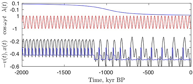
Figure 12. By a slow change of the parameter λ (top blue curve) the system moves from 1:1 synchronization with the forcing through a 2:1 to a 3:1 synchronization. The system crosses the transcritical bifurcation for λ = 0 around t = −1000 kyr. The fast (unobserved) variable x(t) is shown in blue. Compare with the case of the van der Pol oscillator (Figure 8).

The critical manifold {(−λ, v, x)|H(x, v, λ) = 0} is shown in Figure 13. The left panel shows the intersections with the plane λ = 0.1 corresponding to the bifurcation diagram in the left panel in Figure 11, the middle panel shows the intersections with the plane λ = −0.05 corresponding to the bifurcation diagram in the right panel in Figure 11. The right panel shows the trajectory of a few glacial cycles as the period of the cycle change from 41 kyr to 82 kyr at the MPT and further to a 123 kyr period with a slow change of λ (top blue curve in Figure 12).

FIGURE 13

Figure 13. The critical/slow manifold {(−λ, v, x)|H(x, v, λ) = 0} is shown in all three panels. The left panel shows the intersections with the plane λ = 0.1 corresponding to the bifurcation diagram in the left panel in Figure 11, the middle panel shows the intersections with the plane λ = −0.05 corresponding to the bifurcation diagram in the right panel in Figure 11. The right panel shows the trajectory of a few glacial cycles as the period of the cycle increases abruptly at the MPT with a slow change of λ.

This is similar to the scenario moving from a 1:1 through a 2:1 to a 3:1 synchronization for the van der Pol oscillator (Figure 8). Here the system will stay on the lower branch, the glacial state G through an extra oscillation of the forcing, thus the period of the response moves from a 2:1 to a 3:1 resonance (see Figure 12). The dynamics of the 2:1 case are apparent on observing the oscillations of the trajectory on the lower stable manifold in the right panel of Figure 13.

Two dynamical effects are at play in the MPT transition in this model. Firstly, the crossing of the transcritical bifurcation changes the structure of the critical (slow) manifold, secondly, the system has a changing internal oscillation with a period longer than the period of the forcing. The internal oscillation is seen in the autonomous case I(t) = 0 for Figure 14. By changing the parameter β (see Appendix) the model transitions from having stable fixed points to having a stable limit cycle.

FIGURE 14

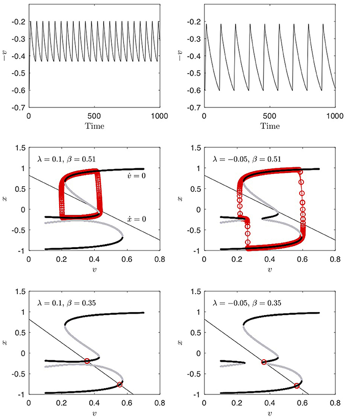
Figure 14. In the autonomous case of no external forcing (I(t) = 0, λ = constant), the system (7) shows internal oscillations both before (λ > 0) and after (λ < 0) the transcritical bifurcation at MPT. The period of the internal oscillation is longer than the period of the forcing (41 kyr): Right top panel shows an internal oscillation of 46 kyr for λ = 0.01, while the left top panel shows an internal oscillation of 110 kyr for λ = −0.05. The middle panels shows the bifurcation diagrams similar to Figure 11. The straight line is the x-nullcline, which crosses the v-nullcline at an unstable branch, thus the fixed point is unstable. By changing β (see Appendix), the x-nullcline moves such that it crosses at a stable branch and the fixed point becomes stable and the limit cycle disappears. This is shown in the bottom panels, with the (multiple) fixed points marked in red.

The synchronization to the forcing frequency in the non-autonomous case has a sharp transition around the transcritical bifurcation λ = 0. Figure 15 shows the synchronization as a function of the forcing amplitude A and the parameter λ. The frequency of the oscillator synchronizes in rational ratio to the forcing frequency ω_F. The colored patches of synchronization are similar to Figure 7. The arrow indicates the change corresponding to the change of α through the MPT shown in Figure 12. The effect of an additional stochastic noise in this model, is to increase variability in the phase of the synchronization, corresponding to jumping between more than one pullback attractor [27] in the 2:1 and 3:1 synchronization situations. For further details we refer the reader to Ashwin and Ditlevsen [16].

FIGURE 15

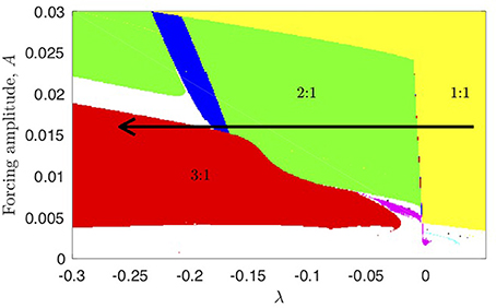
Figure 15. As a function of the forcing amplitude A and the parameter λ the frequency of the oscillator (7) synchronizes in rational ratio to the forcing frequency ω_F. The colored patches of synchronization correspond to the frequency locking shown in Figure 7. The arrow indicates the change corresponding to the change of α through the MPT shown in Figure 12.

7. Summary and Outlook

We have presented some simple nonlinear models of the Pleistocene glacial cycles and the transition at the MPT from a 41 kyr to a 100 kyr response to the astronomical forcing. The apparent 100 kyr cycle after the MPT can be explained without imposing a 100 kyr component (such as the eccentricity cycle) in the forcing. In other words, the MPT is described by an internal reorganization of the response to the forcing, as there is no noticeable difference in the forcing across the MPT. We hypothesize, in accordance with the suggestion by Paillard [17], that the Pleistocene climate can be modeled as a fast-slow system where the slow manifold contains three stable branches, and a generic transcritical transition changes the bifurcation structure on the slow manifold at the MPT.

Understanding the Pleistocene glacial cycles and the MPT is a major challenge in climate science, and progress on this problem may well contribute a large step forward in understanding present day climate change and foreseeing critical transitions in the future Anthropocene climate. The challenge is twofold in the sense that we need to understand both the importance and the coupling between physical components of the climate system and understand the dynamical mechanisms governing the complex interactions between external forcing, internal processes and the different components leading to different timescales in the variability in the climate system.

Phrased a little differently; it might be that by identifying robust dynamical features, such as a bifurcation structure on an effective critical/slow manifold, transitions could be triggered (say, stochastically) by a variety of physical components. Even though the conceptual climate models presented here are very simplistic from a physical point of view, they do show strikingly complex structure in parameter space of possible responses to the astronomical forcing. We have not even considered the quasiperiodic nature of the forcing [27] or chaotic responses to the forcing [37], which add further levels of complexity to the problem. Likewise, we do not consider stochastic modeling of fast chaotic components [38, 39].

The observed Pleistocene climate evolution is currently more or less synonymous with the ocean sediment record (Figure 4), thus the state of the oceanic currents, geographic distribution of vegetation, sea- and land ice, etc. is sparsely known. It is thus often stated that discriminating between alternative models based on reproduction of the one climatic time series is difficult. That is, if the models presented in Figures 8, 10, 12 were forced by a Milankovitch forcing curve and some stochastic forcing, and parameters were tuned to an optimal fit to observations, they might all give a fair reproduction of the record. However, as we have demonstrated, the models presented here do behave differently, and we believe that the higher merits of our model inspires as a benchmark for developing the physical basis for the dynamics.

Author Contributions

PD and PA did the research. PD drafted the co-authored paper.

Conflict of Interest Statement

The authors declare that the research was conducted in the absence of any commercial or financial relationships that could be construed as a potential conflict of interest.

Acknowledgments

PD thanks the Villum Foundation for support. PA thanks the EPSRC for support via ReCoVER (EP/M008495/1). Both authors are grateful for the opportunity to work within the CRITICS Innovative Training Network funded by the European Unions Horizon 2020 research and innovation programme under the Marie Skłodowska-Curie grant agreement No. 643073.

References

1. Taylor KE, Stouffer RJ, Meehl GA. An overview of CMIP5 and the experiment design. Bull Am Meteor Soc. (2012) 93:485–98. doi: 10.1175/BAMS-D-11-00094.1

CrossRef Full Text | Google Scholar

2. Imbrie J, Imbrie JZ. Modelling the climatic response to orbital variations. Science (1980) 207:943–53. doi: 10.1126/science.207.4434.943

CrossRef Full Text | Google Scholar

3. Budyko MI. The effect of solar ratiation variations on the climate of the Earth. Tellus (1969) 21:611–9. doi: 10.3402/tellusa.v21i5.10109

CrossRef Full Text | Google Scholar

4. Sellers WD. A global climatic model based on the energy balance of the earth-atmosphere system. J Appl Meteorol. (1969) 8:392–400.

Google Scholar

5. Abe-Ouchi A, Saito F, Kawamura K, Raymo ME, Okuno J, Takahashi K, et al. Insolation-driven 100,000-year glacial cycles and hysteresis of ice-sheet volume. Nature (2013) 500:190–3. doi: 10.1038/nature12374

PubMed Abstract | CrossRef Full Text | Google Scholar

6. Gildor H, Tziperman E. Sea ice as the glacial cycles' climate switch: role of seasonal and orbital forcing. Paleoceanography (2000) 15:605–15. doi: 10.1029/1999PA000461

CrossRef Full Text | Google Scholar

7. Saltzman B, Maasch KA. A first-order global model of late Cenozoic climate II. Further analysis based on a simplification of the CO2 dynamics. Clim Dyn. (1991) 5:201–10. doi: 10.1007/BF00210005

CrossRef Full Text | Google Scholar

8. Paillard D, Parrenin F. The Antarctic ice sheet and the triggering of deglaciations. Earth Planet Sci Lett. (2004) 227:263–71. doi: 10.1016/j.epsl.2004.08.023

CrossRef Full Text | Google Scholar

9. Huybers P, Carl Wunsch C. Obliquity pacing of the late Pleistocene glacial terminations. Nature (2004) 434:491–4. doi: 10.1038/nature03401

PubMed Abstract | CrossRef Full Text | Google Scholar

10. Ashkenazy Y, Baker DR, Gildor H. Simple stochastic models for glacial dynamics. J Geophys Res. (2005) 110:C02005. doi: 10.1029/2004JC002548

CrossRef Full Text | Google Scholar

11. Shao Z-G, Ditlevsen PD. Contrasting scaling properties of interglacial and glacial climates. Nat Commun. (2016) 7:10951. doi: 10.1038/ncomms10951

PubMed Abstract | CrossRef Full Text | Google Scholar

12. Benzi R, Parisi G, Sutera A, Vulpiani A. Stochasic resonance in climate change. Tellus (1982) 34:10–6. doi: 10.3402/tellusa.v34i1.10782

CrossRef Full Text | Google Scholar

13. Källen E, Crafoord C, Ghil M. Free oscillations in a climate model with ice-sheet dynamics. J Atmos Sci. (1979) 36:2292–303.

Google Scholar

14. LeTreut H, Ghil M. Orbital forcing, climate interactions, and glacial cycles. J Geophys Res. (1983) 88:5167–90. doi: 10.1029/JC088iC09p05167

CrossRef Full Text | Google Scholar

15. Crucifix M. Oscillators and relaxation phenomena in Pleistocene climate theory. Phil Trans R Soc A (2012) 370:1140–65. doi: 10.1098/rsta.2011.0315

PubMed Abstract | CrossRef Full Text | Google Scholar

16. Ashwin P, Ditlevsen P. The middle Pleistocene transition as a generic bifurcation on a slow manifold. Clim Dyn. (2015) 45:2683–95. doi: 10.1007/s00382-015-2501-9

CrossRef Full Text | Google Scholar

17. Paillard D. The timing of Pleistocene glaciations from a simple multiple-state climate model. Nature (1998) 391:378–81. doi: 10.1038/34891

CrossRef Full Text | Google Scholar

18. North GRIP members. High resolution climate record of the northern hemisphere reaching into the last glacial interglacial period. Nature (2004) 431:147–51. doi: 10.1038/nature02805

CrossRef Full Text

19. Dansgaard W, Johnsen SJ, Clausen HB, Dahl-Jensen D, Gundestrup NS, Hammer CU, et al. Evidence for general instability of past climate from a 250-kyr ice-core record. Nature (1993) 364:218–20. doi: 10.1038/364218a0

CrossRef Full Text | Google Scholar

20. Hoffman PF, Kaufman AJ, Halverson GP, Schrag DP. A Neoproterozoic Snowball Earth. Science. (1998) 281:1342–6. doi: 10.1126/science.281.5381.1342

PubMed Abstract | CrossRef Full Text | Google Scholar

21. Berger A. Long-term variations of daily insolation and Quaternary climatic change. J Atmos Sci. (1978) 35:2362–7.

Google Scholar

22. Huybers P. Glacial variability over the last 2ma: an extended depth-derived age model, continuous obliquity pacing, and the Pleistocene progression. Quater. Sci. Rev. (2007) 26:37–55. doi: 10.1016/j.quascirev.2006.07.013

CrossRef Full Text | Google Scholar

23. Tzedakis PC, Crucifix M, Mitsui T, Wolff EW. A simple rule to determine which insolation cycles lead to interglacials. Nature (2017) 542:427–32. doi: 10.1038/nature21364

PubMed Abstract | CrossRef Full Text | Google Scholar

24. Clark PU, Archer D, Pollard D, Blumd JD, Rial JA, Brovkin V, et al. The middle Pleistocene transition: characteristics, mechanisms, and implications for long-term changes in atmospheric pCO2. Quater Sci Rev. (2006) 25:3150–84. doi: 10.1016/j.quascirev.2006.07.008

CrossRef Full Text | Google Scholar

25. Ghil M, Childress S. Topics in Geophysical Fluid Dynamics: Atmospheric Dynamics, Dynamo Theory and Climate Dynamics. Berlin: Springer; Applied Mathematical Sciences, Vol. 60. (1987).

Google Scholar

26. Guckenheimer J, Holmes P. Nonlinear Oscillations, Dynamical Systems, and Bifurcations of Vector Fields. New York, NY: Springer-Verlag (1983).

Google Scholar

27. De Saedeleer B, Crucifix M, Wieczorek S. Is the astronomical forcing a reliable and unique pacemaker for climate? A conceptual model study. Clim Dyn. (2013) 40:273–94. doi: 10.1007/s00382-012-1316-1

CrossRef Full Text | Google Scholar

28. Guckenheimer J, Hoffman K, Weckesser W. The forced van der Pol equation I: the slow flow and its bifurcations SIAM. J Appl Dyn Syst. (2003) 2:1–35. doi: 10.1137/S1111111102404738

CrossRef Full Text | Google Scholar

29. Rasband SN. Chaotic Dynamics of Nonlinear Systems. New York, NY: Wiley (1990).

Google Scholar

30. Raymo ME, Ruddiman WF, Froelich PN. Influence of late Cenozoic mountain building on ocean geochemical cycles. Geology (1988) 16:649–53.

Google Scholar

31. Hönisch B, Hemming NG, Archer D, Siddall M, McManus JF. Atmospheric carbon dioxide concentration across the mid-pleistocene transition. Science (2009) 324:1551–4. doi: 10.1126/science.1171477

PubMed Abstract | CrossRef Full Text | Google Scholar

32. Clark PU, Pollard D. Origin of the middle Pleistocene transition by ice sheet erosion of regolith. Paleoceanography (1998) 13:1–9.

Google Scholar

33. Maasch KA, Saltzman B. A low-order dynamic model of global climate variability over the full Pleistocene. J Geophys Res. (1990) 95:1955–63. doi: 10.1029/JD095iD02p01955

CrossRef Full Text | Google Scholar

34. Engler H, Kaper HG, Kaper TJ, Vo T. Dynamical systems analysis of the Maasch-Saltzman model for glacial cycles. Physica D (2017) 359:1–20. doi: 10.1016/j.physd.2017.08.006

CrossRef Full Text | Google Scholar

35. Ditlevsen PD. The bifurcation structure and noise assisted transitions in the Pleistocene glacial cycles. Paleoceanography (2009) 24:PA3204. doi: 10.1029/2008PA001673

CrossRef Full Text | Google Scholar

36. Arnold VI. Bifurcation Theory and Catastrophe Theory. Heidelberg: Springer-Verlag (1994).

Google Scholar

37. Ashwin P, Camp CD, von der Heydt AS. Chaotic and non-chaotic response to quasiperiodic forcing: limits to predictability of ice ages paced by milankovitch forcing. Dyn Stat Clim Syst. (2018). doi: 10.1093/climsys/dzy002

CrossRef Full Text | Google Scholar

38. Wunsch C. The spectral description of climate change including the 100 ky energy. Clim Dyn. (2003) 20:353–63. doi: 10.1007/s00382-002-0279-z

CrossRef Full Text

39. Ditlevsen PD. Observation of alpha-stable noise and a bistable climate potential in an ice-core record, Geophys. Res Lett. (1999) 26:1441–4. doi: 10.1029/1999GL900252

CrossRef Full Text

Appendix

The model for the middle Pleistocene transition from Ashwin and Ditlevsen [16] in (7) is specified by

$\begin{array}{l}G(x,v)=-(v-v_e(x))/{\tau }_v(x)\\ H(x,v,\lambda )=h_0{tanh}^{-1}(x)+h_{1}x+h_{2}v+h_3+\\ h_4\frac{x+h_6{e}^{-h_{5}v}}{1+h_7{(x+h_8)}^2}+\lambda \end{array}$

where τ_v(x) = (τ_i − τ_G)tanh(μ(x − x_p)) + τ_G and v_e(x) = β(a − x). The parameter values used are (h₀, …, h₈) = (6.9, 7, −2.80847, −50, 5, 0.1, 80, 0.2, −4), a = 0.82, b = 0.51, μ = 3, τ_i = 20, τ_G = 130, and x_p = −0.5.