Power Laws in Stochastic Processes for Social Phenomena: An Introductory Review

Many phenomena with power laws have been observed in various fields of the natural and social sciences, and these power laws are often interpreted as the macro behaviors of systems that consist of micro units. In this paper, we review some basic mathematical mechanisms that are known to generate power laws. In particular, we focus on stochastic processes including the Yule process and the Simon process as well as some recent models. The main purpose of this paper is to explain the mathematical details of their mechanisms in a self-contained manner.

1. Introduction

Many phenomena with power laws have been observed in various fields of the natural and social sciences: physics, biology, earth planetary science, computer science, economics, and so on. These power laws can be interpreted as the macro behaviors of the systems that consist of micro units (i.e., agents, individuals, particles, and so on). In other words, the ensemble of dynamics of these micro units is observed as the behavior of the whole system such as a power law¹. To obtain a deep understanding of the phenomenon for the system, we must first observe the behavior on the macro side, then assume the stochastic dynamics on the micro side, and finally reveal the theoretical method connecting both sides. Thus, the mechanisms generating power laws have been studied as the second and final steps in the study of power laws.

Next, we mathematically define the power law. When the probability density function p(x) for a continuous random variable² $\widehat{X}$ is given by

$\begin{array}{ll}p(x)=C{x}^{-\alpha }(x\ge x_{\text{min}}),& (1)\end{array}$

we say that $\widehat{X}$ satisfies the power law. The exponent α is called the exponent of power law, C is the normalization constant, and x_min is the minimum value that x satisfies the power law. The power law is the only function satisfying the scale-free property [1]

$\begin{array}{ll}p(bx)=f(b)p(x)\text{ for any }b.& (2)\end{array}$

Then we define the cumulative distribution function P_>(x) as

$\begin{array}{ll}{P}_{>}(x):=\text{P}\{\widehat{X}\ge x\}={\displaystyle {\int }_x^{\infty }}p(x)\text{d}x.& (3)\end{array}$

When the probability density function satisfies the power law p(x) = Cx^−α,

$\begin{array}{ll}{P}_{>}(x)\propto x^{-\alpha +1}.& (4)\end{array}$

The behavior of the cumulative distribution function with the power law is a straight line in a log–log plot for x ≥ x_min (Figure 1).

FIGURE 1

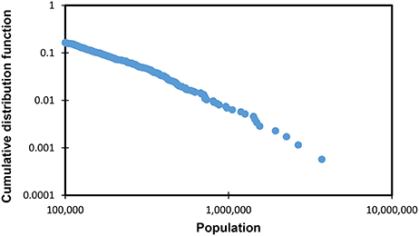
Figure 1. Log–log plot for the cumulative distribution function of the populations of Japanese cities in 2015, with x_min ≃ 100, 000. Data from the basic resident register.

Next, we list some examples of power laws in various phenomena.

(a) Populations of cities [2].

(b) Frequency of use of words [3, 4].

(c) Number of papers published by scientists [5].

(d) Number of citations received by papers [6].

(e) Number of species in biological genera [7, 8].

(f) Number of links on the World Wide Web [9].

(g) Individual wealth and income [10].

(h) Sizes of firms (the number of employees, assets, or market capitalization) [11–17].

(i) Sizes of earthquakes [18].

(j) Sizes of forest fires [19].

Furthermore, we partly list the generating mechanisms that are important for applications, and the phenomena to which they are applied in the above list, such as “mechanism ⇒ phenomena.”

• Growth and preferential attachment:

- Yule process [20] ⇒ (e);

- Simon process [21] ⇒ (a), (b), (c), (e), and (g);

- Barabási–Albert (BA) model [22] ⇒ (d) and (f).

• Stochastic models based on Geometric Brownian motion (GBM):

- GBM with a reflecting wall [23] ⇒ (a), (g), and (h);

- GBM with reset events [24, 25] ⇒ (g).

- Kesten process [26]⇒ (g).

- Generalized Lotka–Volterra (GLV) model [27–29] ⇒ (g);

- Bouchaud–Mézard (BM) model [30] ⇒ (g).

• Combination of exponentials (change of variable) [31] ⇒ (b).

• Self-organized criticality [32] ⇒ (i) and (j).

• Highly optimized tolerance [33, 34] ⇒ (j).

Though there are many other generating mechanisms besides them³, the mechanisms of the above list are particularly well known and widely applied to phenomena in various fields.

In this paper, we focus on the generating mechanisms with the stochastic processes in the above list⁴: the growth and preferential attachment and the stochastic models based on the GBM, which, in particular, are widely applied in social science. In addition, we explain about the combination of exponentials that is related to the mechanism of the Yule process. We mainly give full details of the mathematical formalisms for these mechanisms in self-contained manner, because understanding them is important for researchers in any field to create new models generating power laws in empirical data. The necessary mathematical supplements to understand these mechanisms are given in the Appendix at the end of this paper.

2. Growth and Preferential Attachment

As the name suggests, this mechanism consists of the two characteristics: growth and preferential attachment. In the example of a city, the meanings of growth and preferential attachment are as follows.

• Growth: The number of cities increases.

• Preferential attachment: The more populated cities become, the higher the probability that the population will increase. Namely, it is “the rich get richer” process⁵.

In this section, we deal with the Yule process, the Simon process, and the BA model, which all have these two characteristics. The Yule process generates the power law about the number of species within genera in biology. The Simon process generates the power laws about the frequency of use of a word in a text, the population of cities, and so on (see the list in the Introduction for details). The BA model generates the power law about the number of edges incident to nodes in the network. We now explain in detail how these three mechanisms mathematically generate the power laws.

2.1. Yule Process

The Yule process [20] was invented to model stochastic population growth with the preferential attachment process for the model of speciation in biology. In this process, new species and genera are born by biological mutations that are interpreted as the branchings from the lines of existing species in the evolutionary tree (Figures 2, 3).

FIGURE 2

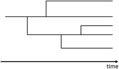
Figure 2. An example of the evolutionary tree of species in the Yule process.

FIGURE 3

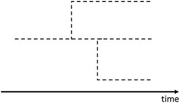
Figure 3. An example of the evolutionary tree of genera in the Yule process.

These branchings occur as Poisson processes and add lines of new genera or species to the evolutionary tree. The Yule process mathematically corresponds to the stochastic process that the numbers of genera and species increase independently by following the linear birth processes (see Appendix A.3)⁶. In other words, we consider the evolutionary tree of species (Figure 2) and that of genera (Figure 3) separately.

In short, the Yule process is the combination of the stochastic processes for the numbers of species and genera (Figure 4) [41, 49, 50].

• The number of species within a genus increases as the linear birth process with the Poisson rate λ_sn_s, where λ_s is a positive constant and n_s is the number of species within the genus at that time.

• The number of genera within a family increases as the linear birth process with the Poisson rate λ_gn_g, where λ_g is a positive constant and n_g is the number of genera within the family at that time.

FIGURE 4

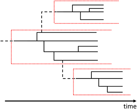
Figure 4. An example of the evolutionary tree for the Yule process. The black solid lines show the branchings of species. The black broken lines show the branchings of genera. One genus is represented by the part surrounded by the red dotted lines. In this figure, though, the probability of branching for a new genus seems to depend on the number of species in the original genus and, in fact, the Poisson rate for branching of a genus is constant in the Yule process.

To obtain the probability distribution of the number of species within genera at a large time⁷, we need the conditional probability distribution of the number of species included in the genus whose age (i.e., the time intervals elapsed since the birth) is t. Let us use r_s(n, t) to denote its conditional probability distribution, where n (∈ ℕ) is the number of species and t (∈ ℝ) is the age of the genus.

First, r_s(1, t) is equivalent to the probability that no new species is born in (a, a + t] after the genus is born⁸ at an arbitrary time a. Accordingly, we obtain r_s(1, t) from (A.2) as

$\begin{array}{ll}{r}_{\text{s}}(1,t)=\text{P}\left\{{\widehat{N}}_{\text{s}}(a+t)-{\widehat{N}}_{\text{s}}(a)=0;\text{ rate }{\lambda }_{\text{s}}\right\}={\text{e}}^{-{\lambda }_{\text{s}}t},& (5)\end{array}$

where ${\widehat{N}}_{\text{s}}(t)$ is the number of species born in (0, t] by the Poisson process with the Poisson rate λ_s.

Second, we calculate r_s(2, t). It is equivalent to the probability that one new species is born in (a, a + t] after the genus is born at an arbitrary time a. Then we assume that one new species is born in the infinitesimal time interval [a + τ₁, a + τ₁ + dτ₁). From (A.2) and (A.3), we obtain the probabilities for one birth or no birth in each of the three divided time intervals:

$\begin{array}{ll}\{\begin{array}{c}\text{ P}\left\{\mathrm{\text{no birth in}}(a,a+{\tau }_1);\text{ rate }{\lambda }_{\text{s}}\right\}={\text{e}}^{-{\lambda }_{\text{s}}{\tau }_1},\hfill \\ \text{ P}\left\{\mathrm{\text{one birth in }}[a+{\tau }_1,a+{\tau }_1+\text{d}{\tau }_1);\text{ rate }{\lambda }_{\text{s}}\right\}=\text{P}\left\{{\widehat{N}}_{\text{s}}(a+{\tau }_1+\text{d}{\tau }_1)-{\widehat{N}}_{\text{s}}(a+{\tau }_1)=1;\text{ rate }{\lambda }_{\text{s}}\right\}\\ ={\text{e}}^{-{\lambda }_{\text{s}}\text{d}{\tau }_1}{\lambda }_{\text{s}}\text{d}{\tau }_1\simeq {\lambda }_{\text{s}}\text{d}{\tau }_1,\\ \text{ P}\left\{\mathrm{\text{no birth in }}[a+{\tau }_1+\text{d}{\tau }_1,a+t);\text{ rate }2{\lambda }_{\text{s}}\right\}={\text{e}}^{-2{\lambda }_{\text{s}}(a+t-{\tau }_1-\text{d}{\tau }_1)}\simeq {\text{e}}^{-2{\lambda }_{\text{s}}(a+t-{\tau }_1)}.\\ \end{array}\hfill & (6)\end{array}$

Integrating the product of these probabilities with respect to τ₁, we obtain

$\begin{array}{ll}\begin{array}{c}{r}_{\text{s}}(2,t)={\displaystyle {\int }_0^t}{\text{e}}^{-{\lambda }_{\text{s}}{\tau }_1}{\lambda }_{\text{s}}{\text{e}}^{-2{\lambda }_{\text{s}}(t-{\tau }_1)}\text{d}{\tau }_1={\text{e}}^{-{\lambda }_{\text{s}}t}(1-{\text{e}}^{-{\lambda }_{\text{s}}t}).\end{array}& (7)\end{array}$

Similarly, r_s(3, t) is given by

$\begin{array}{l}{r}_s(3,t)={{{\displaystyle \int }}^{}}_0^t{\text{e}}^{-{\lambda }_s{\tau }_1}{\lambda }_s\text{d}{\tau }_1{{{\displaystyle \int }}^{}}_{{\tau }_1}^t{\text{e}}^{-2{\lambda }_s({\tau }_2-{\tau }_1)}(2{\lambda }_s){\text{e}}^{-3{\lambda }_s(t-{\tau }_2)}\text{d}{\tau }_2\\ ={\text{e}}^{-{\lambda }_{s}t}{\left(1-{\text{e}}^{-{\lambda }_{s}t}\right)}^2.& (8)\end{array}$

Finally, repeating the same procedure, we obtain r_s(n, t), that is, the conditional probability distribution of the number of species included in the genus at the age of t:

$\begin{array}{l}{r}_s(n,t)={\text{e}}^{-n{\lambda }_{s}t}{\displaystyle \prod _{n-1}^{k=1}\left[{{{\displaystyle \int }}^{}}_{{\tau }_{k-1}}^t{\text{e}}^{{\lambda }_s{\tau }_k}k{\lambda }_s\text{d}{\tau }_k\right]}({\tau }_0:=0)\\ ={\text{e}}^{-n{\lambda }_{s}t}(n-1)!{\displaystyle \prod _{n-1}^{k=1}\left[{{{\displaystyle \int }}^{}}_{x_{k-1}}^{{\text{e}}^{{\lambda }_{s}t}}\text{d}{x}_k\right]}(x_k:={\text{e}}^{{\lambda }_s{\tau }_k},x_0:=1)\\ ={\text{e}}^{-{\lambda }_{s}t}{\left(1-{\text{e}}^{-{\lambda }_{s}t}\right)}^{n-1}.& (9)\end{array}$

Next, let ℓ_g(t) be the probability distribution function for the age of genera at a large time in the linear birth process. It is given by (A.15) as

$\begin{array}{ll}{\ell }_{\text{g}}(t)={\lambda }_{\text{g}}{\text{e}}^{-{\lambda }_{\text{g}}t}.& (10)\end{array}$

Consequently, the probability density of the number of species within genera at a large time, denoted by q(n), is given by integrating the product of the conditional probability distribution of the number of species within genera and the probability density function for the age of genera at a large time:

$\begin{array}{ll}\begin{array}{c}q(n)={\displaystyle {\int }_0^{\infty }}{r}_{\text{s}}(n,t){\ell }_{\text{g}}(t)\text{d}t={\displaystyle {\int }_0^{\infty }}{\text{e}}^{-{\lambda }_{\text{s}}t}{(1-{\text{e}}^{-{\lambda }_{\text{s}}t})}^{n-1}{\lambda }_{\text{g}}{\text{e}}^{-{\lambda }_{\text{g}}t}\text{d}t\\ =\frac{{\lambda }_{\text{g}}}{{\lambda }_{\text{s}}}{\displaystyle {\int }_0^1}{x}^{\frac{{\lambda }_{\text{g}}}{{\lambda }_{\text{s}}}}{(1-x)}^{n-1}\text{d}x(x:={\text{e}}^{-{\lambda }_{\text{s}}t})\hfill \\ =:\frac{{\lambda }_{\text{g}}}{{\lambda }_{\text{s}}}\text{B}\left(\frac{{\lambda }_{\text{g}}}{{\lambda }_{\text{s}}}+1,n\right),\hfill \end{array}& (11)\end{array}$

where the beta function B(a, b) is defined as

$\begin{array}{l}B(a,b):=\frac{\Gamma (a)\Gamma (b)}{\Gamma (a+b)}={\displaystyle {\int }_0^1}{x}^{a-1}{(1-x)}^{b-1}\text{d}x\\ \left(\Gamma (a):={\displaystyle {\int }_0^{\infty }}{t}^{a-1}{\text{e}}^{-t}\text{d}t\right).& (12)\end{array}$

When b takes a large value, the beta function is approximately

$\begin{array}{ll}B(a,b)\propto b^{-a}(b\gg 1).& (13)\end{array}$

Therefore, for a large number of species, the probability distribution of the number of species within genera at a large time satisfies the power law as

$\begin{array}{ll}q(n)\propto n^{-\left(\frac{{\lambda }_{\text{g}}}{{\lambda }_{\text{s}}}+1\right)}(n\gg 1),& (14)\end{array}$

where the exponent of power law is $\frac{{\lambda }_{\text{g}}}{{\lambda }_{\text{s}}}+1$.

2.2. Simon Process

The Simon process [21] is interpreted as a discrete-time stochastic process for the growth in the numbers of urns and balls contained in those urns: an urn and the number of balls in the urn correspond to a word and the number of times that the word is used. In this stochastic process, a certain number of balls are newly added and stochastically distributed to the existing urns containing some balls at each time step. After that, one urn containing a certain number of balls (it need not be the same as the number of balls added above) is also added newly. Repeating this procedure, the number of balls and urns grows stochastically.

We calculate the stationary probability distribution of balls contained in urns at a large time.

First, we define all quantities for the Simon process by using the following notation:

• t (= 0, 1, 2, ⋯ ), discrete time;

• k₀, number of balls contained in each urn in the initial state (before balls are added);

• m, number of balls added at each time step;

• B(t) (= B(0) + t(m + k₀)), total number of balls before balls are distributed at t;

• U(t) (= U(0) + t), number of urns before balls are distributed at t;

• group-(k), group of all the urns containing k balls;

• $\widehat{f}(k,t)$, number of urns belonging to the group-(k) before balls are distributed at t.

Next, we provide the detailed procedure with the stochastic rule as follows (Figure 5).

1. There are U(0) urns containing k₀ balls at the initial time⁹ t = 0.

2. The m balls are newly added at each time step¹⁰.

3. Each of the m balls is distributed once for each group-(k) with the probability $\frac{k\widehat{f}(k,t)}{B(t)}$¹¹.

4. Then the balls distributed to the group-(k) are further distributed to the urns within the group with arbitrary probabilities¹² with the assumption that each urn can only get up to one ball at each time step¹³.

5. At the end of each time step, one urn containing k₀ balls is added.

6. We repeat steps 2–5.

FIGURE 5

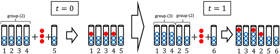
Figure 5. An example of the Simon model with k₀ = 2, U(0) = 4, and m = 3.

Then we can obtain the expectation values of $\text{E}[\widehat{f}(k,t+1)](k\ge k_0)$ from the above stochastic rule as

$\begin{array}{ll}\{\begin{array}{cc}& \text{E}\left[\widehat{f}(k,t+1)\right]=\widehat{f}(k,t)-\frac{mk\widehat{f}(k,t)}{B(t)}+\frac{m(k-1)\widehat{f}(k-1,t)}{B(t)}\\ & (k>k_0),\hfill \\ \hfill & \text{E}\left[\widehat{f}(k_0,t+1)\right]=\widehat{f}(k_0,t)-\frac{m{k}_0\widehat{f}(k_0,t)}{B(t)}+1.\end{array}\hfill & (15)\end{array}$

At a large time t, we can make an approximation $\widehat{f}(k,t)\simeq \text{E}[\widehat{f}(k,t)]$ for k ≥ k₀ and obtain

$\begin{array}{ll}\{\begin{array}{cc}\hfill & \text{E}\left[\widehat{f}(k,t+1)\right]\simeq \text{E}\left[\widehat{f}(k,t)\right]-\frac{mk\text{E}\left[\widehat{f}(k,t)\right]}{B(t)}+\\ & \frac{m(k-1)\text{E}\left[\widehat{f}(k-1,t)\right]}{B(t)}(k>k_0)\\ & \text{E}\left[\widehat{f}(k_0,t+1)\right]\simeq \text{E}\left[\widehat{f}(k_0,t)\right]-\frac{m{k}_0\text{E}\left[\widehat{f}(k_0,t)\right]}{B(t)}+1.\\ \end{array}\hfill & (16)\end{array}$

The probability distribution of the number of balls in urns, denoted by p(k, t), can be represented by $\text{E}[\widehat{f}(k,t+1)]$:

$\begin{array}{ll}p(k,t)=\frac{\text{E}\left[\widehat{f}(k,t)\right]}{U(t)}.& (17)\end{array}$

Consequently, the master equation for p(k, t) is given by

$\begin{array}{ll}\{\begin{array}{cc}\hfill & U(t+1)p(k,t+1)=U(t)p(k,t)-\frac{mkU(t)}{B(t)}p(k,t)+\\ & \frac{m(k-1)U(t)}{B(t)}p(k-1,t)(k>k_0),\\ & U(t+1)p(k_0,t+1)=U(t)p(k_0,t)-\frac{mkU(t)}{B(t)}p(k_0,t)+1.\\ \end{array}& (18)\end{array}$

We are interested in only the stationary distribution function p(k) that is defined as p(k, t) in the limit of large time:

$\begin{array}{ll}p(k):={\displaystyle \underset{t\to \infty }{lim}}p(k,t).& (19)\end{array}$

Then, considering

$\begin{array}{ll}{\displaystyle \underset{t\to \infty }{lim}}\frac{U(t)}{B(t)}=\frac{1}{m+k_0}& (20)\end{array}$

and taking the limit t → ∞ for Equation (18), we obtain

$\begin{array}{ll}\{\begin{array}{cc}\hfill & p(k)=\frac{k-1}{k+1+\frac{k_0}{m}}p(k-1)(k>k_0),\\ \hfill & p(k_0)=\frac{m+k_0}{k_0(m+1)+m}.\\ \end{array}& (21)\end{array}$

We can solve these equations recursively:

$\begin{array}{ll}\begin{array}{c}p\left(k\right)=\frac{\left(k-1\right)\left(k-2\right)\cdots k_0}{\left(k+1+\frac{k_0}{m}\right)\left(k+\frac{k_0}{m}\right)\cdots \left(k_0+2+\frac{k_0}{m}\right)}p\left(k_0\right)\hfill \\ =\frac{\left(k-1\right)\left(k-2\right)\cdots k_0}{\left(k-1+\alpha \right)\left(k-2+\alpha \right)\cdots \left(k_0+\alpha \right)}p\left(k_0\right)\left(\alpha :=2+\frac{k_0}{m}\right)\hfill \\ =\frac{\Gamma \left(k\right)\Gamma \left(k_0+\alpha \right)}{\Gamma \left(k_0\right)\Gamma \left(k+\alpha \right)}p\left(k_0\right)\hfill \\ =\frac{\text{B}\left(k,\alpha \right)}{\text{B}\left(k_0,\alpha \right)}p\left(k_0\right).\hfill \end{array}& (22)\end{array}$

For the large k, the stationary probability distribution of the number of balls in urns satisfies the power law as

$\begin{array}{ll}p\left(k\right)\propto k^{-\left(\frac{k_0}{m}+2\right)}\left(k\gg 1\right),& (23)\end{array}$

where the exponent of power law is $\frac{k_0}{m}+2$.

2.3. Barabási–Albert Model

The BA model [22] is one of the scale-free network models for the growth in the number of nodes and edges. Mathematically, the BA model can be interpreted as a special case of the Simon model. In particular, the nodes and edges in the BA model correspond to the urns and balls in the Simon model, respectively (Figure 6). In this model, one node with a certain number of edges are newly added at each time step. Then following a stochastic rule, the edges of new node are connected to the existing nodes. Repeating this procedure, the number of nodes and edges grows stochastically.

FIGURE 6

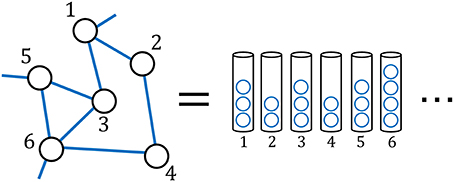
Figure 6. An example of equivalence between a networks and the urns containing balls.

We calculate the stationary probability distribution of edges connecting to nodes at a large time. First, we define all quantities for the BA model by using the following notation:

• t (= 0, 1, 2, ⋯ ), discrete time;

• k₀, number of edges that the additional new node has;

• B(t) (= B(0) + 2tk₀), total number of degrees in the network before the new node is added at t;

• U(t) (= U(0) + t), number of nodes in the network before the new node is added at t;

• $\widehat{f}(k,t)$, number of nodes with the degree k before the new node is added at t;

• ${\widehat{k}}_i(t)$, number of the edges of node-i (where i is the label of the node) before the new node is added at t.

Next, we give the detailed procedure with the stochastic rule for the BA model as follows (Figure 7).

1. At the initial time t = 0, there is an arbitrary connected network with U(0) nodes that are all connected to nodes other than themselves¹⁴.

2. One new node with k₀ edges is added¹⁵.

3. The k₀ edges of the new node are connected to the existing nodes following the stochastic rule^16,17: the probability that one edge is connected to the existing node-i is $\frac{{\widehat{k}}_i(t)}{B(t)}$ under the assumption that each node can only connect to one node at each time step¹⁸.

4. We repeat steps 2 and 3.

FIGURE 7

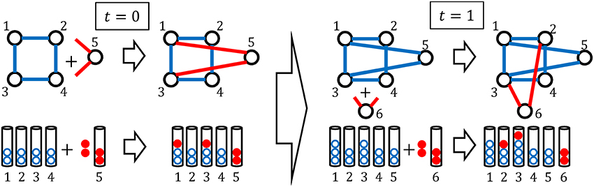
Figure 7. An example of the BA model with k₀ = 2 and U(0) = 4 and the Simon model equivalent to it.

Consequently, we obtain the same master equation for the probability distribution of edges as (18) with m = k₀:

$\begin{array}{ll}\{\begin{array}{cc}\hfill & U(t+1)p(k,t+1)=U(t)p(k,t)-\frac{k_{0}kU(t)}{B(t)}p(k,t)+\\ & \frac{k_0(k-1)U(t)}{B(t)}p(k-1,t)(k>k_0),\\ & U(t+1)p(k_0,t+1)=U(t)p(k_0,t)-\frac{k_{0}kU(t)}{B(t)}p(k_0,t)+1.\\ \end{array}& (24)\end{array}$

We can solve this master equation and obtain the stationary distribution function $p(k):=\underset{t\to \infty }{lim}p(k,t)$ for the large k from Equations (21–23):

$\begin{array}{ll}p(k)\propto k^{-\alpha }\left(\alpha :=2+\frac{k_0}{k_0}=3\right),& (25)\end{array}$

where the exponent of power law is 3.

3. Stochastic Models Based On Geometric Brownian Motion

In this section we look at five stochastic processes, generating power laws, which can be represented by the stochastic differential equations (SDEs). They all are mathematically based on the GBM and accompanied by a constraint (i.e., additional condition) or additional terms to the SDE. The constraints correspond to a reflecting wall¹⁹ as a boundary condition [23], and reset events (i.e., birth and death process²⁰) [25]. The stochastic processes with additional terms to the SDE of GBM are the Kesten process, the GLV model, and the BM model. Though the effect of additional term to the GMB in the Kesten process is similar to a reflecting wall, those of the GLV model and BM model correspond to the interactions between particles, agents, or individuals. We mainly explain the mathematical formalisms and properties of these qualitatively different stochastic processes.

3.1. Geometric Brownian Motion

The GBM, on which many models for power laws are based, is one of the most important stochastic processes. It is mathematically defined by the SDE

$\begin{array}{ll}\text{d}\widehat{X}(t)=\mu \widehat{X}(t)\text{d}t+\sigma \widehat{X}(t)\text{d}\widehat{B}(t),& (26)\end{array}$

where $\widehat{B}(t)$ is a standard Brownian motion, μ is the drift, and σ is the volatility.

The SDE (Equation 26) gives us the partial differential equation (PDE), that is, the Fokker–Planck equation (FPE) [51]:

$\begin{array}{ll}\frac{\partial p(x,t)}{\partial t}=-\frac{\partial }{\partial x}\left\{\mu xp(x,t)\right\}+\frac{{\partial }^2}{\partial x^2}\left\{\frac{{\sigma }^2{x}^2}{2}p(x,t)\right\},& (27)\end{array}$

where p(x, t) is the probability density function. The solution of Equation (27) with the initial distribution p(x, 0) = δ(x − x₀) is

$\begin{array}{ll}p(x,t)=\frac{1}{x\sqrt{2\pi {\sigma }^{2}t}}exp\left[-\frac{{\left\{logx-log{x}_0-(\mu -\frac{{\sigma }^2}{2})t\right\}}^2}{2{\sigma }^{2}t}\right],& (28)\end{array}$

where x₀ is the initial position of the particle. This solution is the log-normal distribution where the expectation value and variance are

$\begin{array}{ll}\text{E}\left[\widehat{x}\right]=x_0{\text{e}}^{\mu t},\text{ Var}\left[\widehat{x}\right]={x_0}^2{\text{e}}^{2\mu t}({\text{e}}^{{\sigma }^{2}t}-1).& (29)\end{array}$

In the limit t → ∞, the log-normal distribution never converges to the stationary solution. To obtain it, therefore, we need to impose some additional conditions on the SDE (Equation 26) or modify the SDE itself. We introduce the conditions and modifications in the following sections.

3.2. GBM With a Reflecting Wall

We consider the GBM with the reflecting wall (see Appendix A.5 for details). The stationary solution p(x) for the FPE (Equation 27) is defined by

$\begin{array}{ll}\frac{\partial p(x)}{\partial t}=0,& (30)\end{array}$

which is equivalent to the second-order ordinary differential equation (ODE):

$\begin{array}{ll}0=-\frac{\text{d}}{\text{d}x}\left\{\mu xp(x)\right\}+\frac{{\text{d}}^2}{\text{d}{x}^2}\left\{\frac{{\sigma }^2{x}^2}{2}p(x)\right\}.& (31)\end{array}$

As a result, we obtain the first-order ODE:

$\begin{array}{ll}\mu xp(x)-\frac{\text{d}}{\text{d}x}\left\{\frac{{\sigma }^2{x}^2}{2}p(x)\right\}=D,& (32)\end{array}$

where D is an arbitrary constant. We take D = 0 to obtain a normalizable power-law probability distribution. The solution of Equation (32) with D = 0 is

$\begin{array}{ll}p(x)=C{x}^{-\alpha }\left(C:=p(x_0){x_0}^{\alpha },\alpha :=2-\frac{2\mu }{{\sigma }^2}\right),& (33)\end{array}$

where x₀ is an arbitrary constant. For this stationary solution p(x) to exist, it must satisfy the normalization condition:

$\begin{array}{ll}1={\displaystyle {\int }_{x_{\text{min}}}^{x_{\text{max}}}}p(x)\text{d}x.& (34)\end{array}$

We set the reflecting wall at x = x_min(> 0) and take x_max = ∞. The existence of the reflecting wall is mathematically equivalent to the conditions $\widehat{X}(t)>x_{\text{min}}$ and p(x) = 0 for x < x_min. Then we assume α > 1. The normalization condition

$\begin{array}{ll}1={\displaystyle {\int }_{x_{\text{min}}}^{\infty }}p(x)\text{d}x=\frac{C}{\alpha -1}{(x_{\text{min}})}^{-\alpha +1}& (35)\end{array}$

determines the constant C as

$\begin{array}{ll}C=(\alpha -1){(x_{\text{min}})}^{-\alpha +1}.& (36)\end{array}$

Thus, we have the normalized stationary solution

$\begin{array}{ll}p(x)=(\alpha -1){(x_{\text{min}})}^{-\alpha +1}{x}^{-\alpha }\left(\alpha =2-\frac{2\mu }{{\sigma }^2}>1\right),& (37)\end{array}$

where the exponent of power law is $2-\frac{2\mu }{{\sigma }^2}$.

Next, we generalize this formalism from the GBA to the Itô process which can have the stationary solution [52]:

$\begin{array}{ll}\text{d}\widehat{X}(t)=a(\widehat{X}(t))\text{d}t+b(\widehat{X}(t))\text{d}\widehat{B}(t).& (38)\end{array}$

The stationary solution (see Appendix A.5 for details) is given by

$\begin{array}{ll}p(x)=\frac{C}{b{(x)}^2}exp\left[{\displaystyle {\int }_{x_0}^x}\frac{2a(x^{\prime })}{b{(x^{\prime })}^2}\text{d}{x}^{\prime }\right],& (39)\end{array}$

where C is the normalization constant. Following Yakovenko and Rosser [53] and Banerjee and Yakovenko [54], we take a(x) and b(x) as

$\begin{array}{ll}a(x)=\mu x+{\mu }^{*},b(x)=\sigma \sqrt{2(x^2+{x^{*}}^2)},& (40)\end{array}$

which is interpreted as a kind of qualitative combination of the generalized Wiener process²¹ and GBM. Consequently, we obtain the stationary solution

$\begin{array}{ll}p(x)=C{\left[1+{\left(\frac{x}{x^{*}}\right)}^2\right]}^{\frac{\mu }{2{\sigma }^2}-1}exp\left[\frac{{\mu }^{*}}{{\sigma }^2{x}^{*}}arctan\left(\frac{x}{x^{*}}\right)\right].& (41)\end{array}$

For x ≪ x*, the stationary solution becomes the exponential distribution while for the large x, it satisfies the power law as

$\begin{array}{ll}p(x)\propto x^{-\left(2-\frac{\mu }{{\sigma }^2}\right)}(x\gg x^{*}),& (42)\end{array}$

where the exponent of power law is $2-\frac{\mu }{{\sigma }^2}$.

3.3. GBM With Reset Events

We consider the particles that follow the GBM with the reset events, that is, the birth and death events²². For simplicity, we assume that particles can disappear with a certain probability by following a Poisson process and immediately appear at a point so that the number of particles is conserved. By these reset events, the FPE (Equation 27) is changed into

$\begin{array}{l}\frac{\partial p(x,t)}{\partial t}=-\frac{\partial }{\partial x}\left\{\mu xp(x,t)\right\}+\frac{{\partial }^2}{\partial x^2}\left\{\frac{{\sigma }^2{x}^2}{2}p(x,t)\right\}\\ +\eta \delta (x-x^{*})-\eta p(x,t),& (43)\end{array}$

where η is the probability for a particle in [x, x + dx) to disappear per the time interval dt, and the particle reappears immediately at x = x*(> 0). Accordingly, we obtain the second-order ODE for the stationary solution p(x):

$\begin{array}{ll}0=-\frac{\text{d}}{\text{d}x}\left\{\mu xp(x)\right\}+\frac{{\text{d}}^2}{\text{d}{x}^2}\left\{\frac{{(\sigma x)}^2}{2}p(x)\right\}-\eta p(x),& (44)\end{array}$

which is held except for x = x*. To solve this equation easily, we change the variable x into y: = logx. The new probability density function q(y) is determined by

$\begin{array}{ll}q(y)=p(x)\left|\frac{\text{d}x}{\text{d}y}\right|.& (45)\end{array}$

Then we obtain the ODE for q(y):

$\begin{array}{ll}0=-\left(\mu -\frac{{\sigma }^2}{2}\right)\frac{\text{d}q(y)}{\text{d}y}+\frac{{\sigma }^2}{2}\frac{{\text{d}}^{2}q(y)}{\text{d}{y}^2}-\eta q(y),& (46)\end{array}$

except for y = y* (y*: = logx*). The general solution of this second-order ODE is

$\begin{array}{ll}\{\begin{array}{cc}\hfill & q\left(y\right)=C_1{\text{e}}^{{\lambda }_{1}y}+C_2{\text{e}}^{{\lambda }_{2}y},\\ & {\lambda }_1=\frac{1}{{\sigma }^2}\left(\mu -\frac{{\sigma }^2}{2}+\sqrt{{\left(\mu -\frac{{\sigma }^2}{2}\right)}^2+2{\sigma }^2\eta }\right)>0,\\ & {\lambda }_2=\frac{1}{{\sigma }^2}\left(\mu -\frac{{\sigma }^2}{2}-\sqrt{{\left(\mu -\frac{{\sigma }^2}{2}\right)}^2+2{\sigma }^2\eta }\right)<0,\end{array}& (47)\end{array}$

where C₁ and C₂ are the arbitrary constants determined by the normalization condition:

$\begin{array}{ll}1={\displaystyle {\int }_0^{\infty }}p(x)\text{d}x={\displaystyle {\int }_{-\infty }^{\infty }}q(y)\text{d}y.& (48)\end{array}$

To normalize the solution (Equation 47), we impose the boundary conditions q(∞) = q(−∞) = 0, which result in C₁ = 0 for y ≥ y* and C₂ = 0 for y < y*, that is,

$\begin{array}{ll}q(y)=\{\begin{array}{cc}& C_1{\text{e}}^{{\lambda }_{1}y}(y<y^{*}),\\ & C_2{\text{e}}^{{\lambda }_{2}y}(y\ge y^{*}).\\ \end{array}& (49)\end{array}$

Accordingly, the normalization condition

$\begin{array}{ll}1={\displaystyle {\int }_{-\infty }^{y^{*}}}{C}_1{\text{e}}^{{\lambda }_{1}y}\text{d}y+{\displaystyle {\int }_{y^{*}}^{\infty }}{C}_2{\text{e}}^{{\lambda }_{2}y}\text{d}y& (50)\end{array}$

and the continuous condition at y = y*, namely, $C_1{\text{e}}^{{\lambda }_1{y}^{*}}=C_2{\text{e}}^{{\lambda }_2{y}^{*}}$ give us the normalized solution of Equation (46) as

$\begin{array}{ll}q(y)=\{\begin{array}{cc}& \frac{{\lambda }_1{\lambda }_2}{{\lambda }_2-{\lambda }_1}{\text{e}}^{{\lambda }_1(y-y^{*})}(y<y^{*}),\\ & \frac{{\lambda }_1{\lambda }_2}{{\lambda }_2-{\lambda }_1}{\text{e}}^{{\lambda }_2(y-y^{*})}(y\ge y^{*}).\\ \end{array}& (51)\end{array}$

Consequently, we obtain the solution of Equation (44):

$\begin{array}{ll}p(x)=\frac{q(logx)}{x}=\{\begin{array}{cc}\hfill & \frac{{\lambda }_1{\lambda }_2}{{\lambda }_2-{\lambda }_1}{(x^{*})}^{-{\lambda }_1}{x}^{{\lambda }_1-1}(0<x<x^{*}),\hfill \\ \hfill & \frac{{\lambda }_1{\lambda }_2}{{\lambda }_2-{\lambda }_1}{(x^{*})}^{-{\lambda }_2}{x}^{{\lambda }_2-1}(x^{*}\le x),\hfill \end{array}& (52)\end{array}$

which is called the double Pareto distribution [25]. The exponents of the power law are 1 − λ₁ and 1 − λ₂.

Next, we derive the probability density function (Equation 52) by another method as follows [56]. The lifetimes of particles are independently distributed with the exponential distribution as ${\ell }_{\text{LT}}(\tau )=\eta {\text{e}}^{-\eta \tau }$, because the death events occur as a Poisson process, with rate η, which have the time-reversal symmetry property. Accordingly, the ages of particles (i.e., the time intervals elapsed since the birth of them) at a large time are also independently distributed with the exponential distribution:

$\begin{array}{ll}{\ell }_{\text{A}}(t)=\eta {\text{e}}^{-\eta t}.& (53)\end{array}$

The probability density function of particles of age t as the conditional probability distribution is given by the log-normal distribution (Equation 28) with $x_0=x^{*}$. Consequently, the probability density function of the coordinate of particle at a large time, denoted by p(x), is given by integrating the product of Equations (53) and (28):

$\begin{array}{ll}p(x)={\displaystyle {\int }_0^{\infty }}\eta {\text{e}}^{-\eta t}\frac{1}{x\sqrt{2\pi {\sigma }^{2}t}}exp\left[-\frac{{\left\{logx-log{x}^{*}-(\mu -\frac{{\sigma }^2}{2})t\right\}}^2}{2{\sigma }^{2}t}\right]\text{d}t.& (54)\end{array}$

We can calculate this with the change of variable u²: = t and the identity [35]

$\begin{array}{ll}{\displaystyle {\int }_0^{\infty }}exp\left(-a{u}^2-\frac{b}{u^2}\right)\text{d}u=\frac{1}{2}\sqrt{\frac{\pi }{a}}exp\left(-2\sqrt{ab}\right).& (55)\end{array}$

Thus, we obtain the same result with Equation (52)²³ without solving the ODE (Equation 44).

3.4. Kesten Process

The Kesten process [26] is defined as a stochastic process whereby an additional term is added to the SDE of the GBM; namely, the SDE is represented by

$\begin{array}{ll}\text{d}\widehat{X}(t)=\mu \widehat{X}(t)\text{d}t+\sigma \widehat{X}(t)\text{d}\widehat{B}(t)+ĉ\text{d}t,& (56)\end{array}$

where ĉ, in the additional term, is a random variable. We can expect that the additional term prevents $\widehat{X}(t)$ from decreasing toward −∞ in a similar way as the reflecting wall in section 3.2

Here, we simply take ĉ as a positive constant: ĉ = c (> 0). We then obtain the FPE for the probability density function:

$\begin{array}{ll}\frac{\partial p(x,t)}{\partial t}=-\frac{\partial }{\partial x}\left\{(\mu x+c)p(x,t)\right\}+\frac{{\partial }^2}{\partial x^2}\left\{\frac{{\sigma }^2{x}^2}{2}p(x,t)\right\}.& (57)\end{array}$

The ODE for the stationary solution p(x) is given by

$\begin{array}{ll}0=-\frac{\text{d}}{\text{d}x}\left\{(\mu x+c)p(x)\right\}+\frac{{\text{d}}^2}{\text{d}{x}^2}\left\{\frac{{(\sigma x)}^2}{2}p(x)\right\}.& (58)\end{array}$

Consequently, we obtain the normalized stationary solution of Equation (58)²⁴:

$\begin{array}{ll}p(x)=\frac{1}{\Gamma \left(\alpha -1\right)}{\left(\frac{2c}{{\sigma }^2}\right)}^{\alpha -1}exp\left[-\frac{2c}{{\sigma }^{2}x}\right]x^{-\alpha }\left(\alpha :=2-\frac{2\mu }{{\sigma }^2}\right),& (59)\end{array}$

where Γ(α) is the gamma function defined in Equation (12). For the large x, the stationary solution satisfies the power law given as

$\begin{array}{ll}p(x)\propto x^{-\beta }(x\gg 1),& (60)\end{array}$

where the exponent of the power law is $2-\frac{2\mu }{{\sigma }^2}$. Although c, in the additional term, achieves the stationary state, it is independent of the exponent. It is worth noting that the exponent of the power law is affected not by the constant c of the additional term, but by the drift μ and volatility σ of the GBM. The additional term affects only the lower tail of the probability density function. Even for c as a random variable, these properties are invariant.

3.5. Generalized Lotka–Volterra Model

The GLV model was introduced for the analysis of individual income distribution. We consider the dynamical system composed of N agents (individuals) with incomes that grow by the GBM process and have the interactions for the redistribution of wealth [27–29]. The GLV model is represented by the system of SDEs called the GLV equations:

$\begin{array}{l}\text{d}{\widehat{X}}_i(t)=\mu {\widehat{X}}_i(t)\text{d}t+\sigma {\widehat{X}}_i(t)\text{d}{\widehat{B}}_i(t)+\xi Û(t)\text{d}t-\eta Û(t){\widehat{X}}_i(t)\text{d}t\\ \left(Û(t):=\frac{1}{N}{\displaystyle \sum _{i=1}^N}{\widehat{X}}_i(t),\xi >0\right),& (61)\end{array}$

where ${\widehat{X}}_i(t)$ is the individual income of agent i (i = 1, 2, ⋯ , N) at t, and Û(t) is the average income for the whole system. To keep ${\widehat{X}}_i(t)>0$, the third term in RHS of Equation (61) redistributes a fraction of the total income for the whole system. This term can be interpreted as the effect of a tax or social security policy. The fourth term controls the growth of whole system and can be interpreted as the effect of finiteness of resources, technological innovations, wars, natural disasters, and so on.

The GLV equations have no stationary solution, and the total income for the entire system is not constant with time. Here, we introduce the new random variable as the relative value:

$\begin{array}{ll}{Ŷ}_i(t):=\frac{{\widehat{X}}_i(t)}{Û(t)}.& (62)\end{array}$

Then we obtain the SDEs for Ŷ_i(t) as

$\begin{array}{ll}\begin{array}{c}\text{d}{Ŷ}_i(t)=\frac{\text{d}{\widehat{X}}_i(t)}{Û(t)}-\frac{{\widehat{X}}_i(t)\text{d}Û(t)}{Û{(t)}^2}\hfill \\ =\xi (1-{Ŷ}_i(t))\text{d}t+\sigma {Ŷ}_i(t)\text{d}{\widehat{B}}_i(t)-\frac{\sigma {Ŷ}_i(t)}{NÛ(t)}{\displaystyle \sum _{i=1}^N}{\widehat{X}}_i(t)\text{d}{\widehat{B}}_i(t),\end{array}& (63)\end{array}$

where the last term in the second row is of the order $N^{-\frac{1}{2}}$, because the standard deviation of $\sum _{i=1}^N{\widehat{X}}_i(t)\text{d}{\widehat{B}}_i(t)$ is of the order $\sqrt{N}$.

We then take the large N limit as the mean field approximation and obtain the new system of SDEs:

$\begin{array}{ll}\text{d}{Ŷ}_i(t)\simeq -\xi {Ŷ}_i(t)\text{d}t+\sigma {Ŷ}_i(t)\text{d}{\widehat{B}}_i(t)+\xi \text{d}t,& (64)\end{array}$

which has the same form as the SDE of Equation (56) in the Kesten process. We can use the result of Equation (59) to obtain the normalized stationary probability density:

$\begin{array}{ll}q(y)=\frac{1}{\Gamma \left(\alpha -1\right)}{\left(\frac{2\xi }{{\sigma }^2}\right)}^{\alpha -1}exp\left[-\frac{2\xi }{{\sigma }^{2}y}\right]y^{-\alpha }\left(\alpha :=2+\frac{2\xi }{{\sigma }^2}\right).& (65)\end{array}$

For large y, the stationary solution satisfies the power law as follows:

$\begin{array}{ll}q(y)\propto y^{-\alpha }(y\gg 1),& (66)\end{array}$

where the exponent of the power law is $2+\frac{2\xi }{{\sigma }^2}$. Consequently, by a change of variables, and the mean field approximation, the GLV model with interactions gives us the same result as that obtained by the Kesten process without interactions.

3.6. Bouchaud–Mézard Model

The BM model was introduced for the analysis of wealth distribution [30, 57–59]. We suppose there is an economic network composed of N agents (individuals) with wealth that grows by the GBM process and is redistributed by the exchanges between agents. The BM model is represented by the system of SDEs as follows:

$\begin{array}{ll}\text{d}{\widehat{X}}_i(t)=\mu {\widehat{X}}_i(t)\text{d}t+\sigma {\widehat{X}}_i(t)\text{d}{\widehat{B}}_i(t)+{\displaystyle \sum _{j(\ne i)}}{a}_{ij}({\widehat{X}}_j(t)-{\widehat{X}}_i(t))\text{d}t& (67)\end{array}$

where ${\widehat{X}}_i(t)$ is the individual wealth of agent i at t, and a_ij is the positive exchange rate between agent i and j. The wealth is exchanged by the third term in RHS of Equation (67), which can be interpreted as a kind of trading in the economic network.

For simplicity, we take a_ij as the constant $\frac{a}{N}(>0)$ in preparation for the mean field approximation. Here, we again introduce the new random variables as the average of wealth and the relative value:

$\begin{array}{ll}{Ŷ}_i(t):=\frac{{\widehat{X}}_i(t)}{Û(t)}\left(Û(t):=\frac{1}{N}{\displaystyle \sum _{i=1}^N}{\widehat{X}}_i(t)\right).& (68)\end{array}$

We then obtain the SDEs for Ŷ_i(t) in the mean field approximation:

$\begin{array}{ll}\begin{array}{c}\text{d}{Ŷ}_i(t)=\frac{\text{d}{\widehat{X}}_i(t)}{Û(t)}-\frac{{\widehat{X}}_i(t)\text{d}Û(t)}{Û{(t)}^2}\hfill \\ \simeq -a{Ŷ}_i(t)\text{d}t+\sigma {Ŷ}_i(t)\text{d}{\widehat{B}}_i(t)+a\text{d}t,\end{array}& (69)\end{array}$

which has the same form as the SDE of Equation (64) in the LV model. Consequently, we obtain the normalized stationary solution:

$\begin{array}{ll}q(y)=\frac{1}{\Gamma (\alpha -1)}{\left(\frac{2a}{{\sigma }^2}\right)}^{\alpha -1}exp\left[-\frac{2a}{{\sigma }^{2}y}\right]y^{-\alpha }\left(\alpha :=2+\frac{2a}{{\sigma }^2}\right).& (70)\end{array}$

For large y, the stationary solution satisfies the following power law:

$\begin{array}{ll}q(y)\propto y^{-\alpha }(y\gg 1),& (71)\end{array}$

where the exponent of the power law is $2+\frac{2a}{{\sigma }^2}$. It is worth noting that though the forms of the additional terms in the GLV model and BM model are quantitatively different from those of the Kesten process, the results are eventually the same in the mean field approximation.

4. Combination of Exponentials

When we have a probability density or distribution function for a random variable, we can obtain a new distribution by a change of variable. In particular, we can obtain a power law function from an exponential distribution by taking a new variable as the exponential function of the original variable. This mechanism was used to interpret the observed power law for the frequency of use of words with the assumption of random typings on a typewriter [31]. In this section, firstly we formalize this mechanism. Then we give the examples of applications to the Yule process and critical phenomena in physics.

4.1. General Formalism

Suppose the probability density function for a continuous random variable x is given by

$\begin{array}{ll}p(x)=A{\text{e}}^{ax}(A>0).& (72)\end{array}$

We change the variable x into the new variable y as

$\begin{array}{ll}y=B{\text{e}}^{bx}(B>0).& (73)\end{array}$

Thus the new probability density function q(y) is obtained as

$\begin{array}{ll}q(y)=p(x)\left|\frac{\text{d}x}{\text{d}y}\right|=\frac{A}{|b|B^{\frac{a}{b}}}{y}^{\frac{a}{b}-1}\propto y^{\frac{a}{b}-1},& (74)\end{array}$

where the exponent of power law is $\frac{a}{b}-1$.

Similarly, when the x is a discrete random variable, the new probability distribution function q(y) is obtained as

$\begin{array}{ll}q(y)=p(x)=\frac{A}{B^{\frac{a}{b}}}{y}^{\frac{a}{b}}\propto y^{\frac{a}{b}},& (75)\end{array}$

where the exponent of power law is $\frac{a}{b}$.

4.2. Application to Yule Process

The power law of the Yule process can be interpreted using a combination of exponentials with a rough approximation [41]. Firstly, by changing the Poisson rate λ_s into λ_g in (A.15), the probability density function of the age of genera at a large time is obtained as

$\begin{array}{ll}p(t)={\lambda }_{\text{g}}{\text{e}}^{-{\lambda }_{\text{g}}t}.& (76)\end{array}$

Then, from (A.12) with n_s0 = 1, we approximately obtain the number of species within the genus of age t as

$\begin{array}{ll}n(t)\simeq \text{E}\left[{\widehat{N}}_{\text{s}}(t)\right]={\text{e}}^{{\lambda }_{\text{s}}t}.& (77)\end{array}$

Finally, taking A = λ_g, a = −λ_g, B = 1, and b = λ_s in Equation (74), the probability density function of the number of species within genera is

$\begin{array}{ll}q(n)=\frac{{\lambda }_{\text{g}}}{{\lambda }_{\text{s}}}{n}^{-\left(\frac{{\lambda }_{\text{g}}}{{\lambda }_{\text{s}}}+1\right)},& (78)\end{array}$

where the exponent of power law is $\frac{{\lambda }_{\text{g}}}{{\lambda }_{\text{s}}}+1$. This exponent coincides with Equation (14). Thus the generating mechanism of power law in the Yule process can be roughly interpreted as a combination of exponentials as well.

4.3. Application to Critical Phenomena

It is well-known that in certain critical phenomena, some physical quantities (e.g., correlation length, susceptibility, and specific heat) take the form of power functions of the reduced temperature $\frac{T-T_{\text{c}}}{T_{\text{c}}}$ near the critical temperature T_c. By the renormalization group analysis [60], this property can be interpreted as emerging from a combination of exponentials [41].

We consider two physical quantities x and y whose scaling dimensions are d_x and d_y, respectively. When we perform the scale transformation (i.e., renormalization group transformation) by the scaling factor b near the critical point, we suppose that x and y are multiplied by λ_x and λ_y, respectively. By the dimensional analysis, we obtain

$\begin{array}{ll}{\lambda }_x=b^{{\text{d}}_x},{\lambda }_y=b^{{\text{d}}_y}\left(\frac{log{\lambda }_y}{log{\lambda }_x}=\frac{{\text{d}}_y}{{\text{d}}_x}\right).& (79)\end{array}$

Then we obtain geometric progressions for the transformed x and y:

$\begin{array}{ll}\{\begin{array}{cc}& x:x_0\to {\lambda }_x{x}_0\to {({\lambda }_x)}^2{x}_0\to \cdots ,\\ & y:y_0\to {\lambda }_y{y}_0\to {({\lambda }_y)}^2{y}_0\to \cdots ,\end{array}& (80)\end{array}$

where x₀ and y₀ are the initial values of the transformation. Let us denote x and y transformed n times by x_n and y_n, respectively. Accordingly, x_n and y_n are defined as

$\begin{array}{ll}\{\begin{array}{cc}& x_n:={({\lambda }_x)}^n{x}_0=x_0{\text{e}}^{(log{\lambda }_x)n},\\ & y_n:={({\lambda }_y)}^n{y}_0=y_0{\text{e}}^{(log{\lambda }_y)n},\end{array}& (81)\end{array}$

which constitute a combination of exponentials. Therefore, taking A = y₀, a = logλ_y, B = x₀, and b = logλ_x in Equation (75), we can write down y_n as a function of x_n as

$\begin{array}{ll}{y}_n=y_0{\left(\frac{x_n}{x_0}\right)}^{\frac{log{\lambda }_y}{log{\lambda }_x}}\propto {x_n}^{\frac{{\text{d}}_y}{{\text{d}}_x}},& (82)\end{array}$

where the exponent of power law is $-\frac{d_y}{d_x}$. We emphasize that this is a simple consequence of the dimensional analysis.

Furthermore, if y : = p(x), the two geometric progressions (Equation 80) lead to

$\begin{array}{ll}{\lambda }_{y}y=p({\lambda }_{x}x),& (83)\end{array}$

which satisfies the scale-free property (Equation 2) with b = λ_x and f(b) = λ_y. Namely, the two geometric progressions, equivalent to a combination of exponentials by the scale transformation, assures that the scale-free property holds²⁵.

5. Conclusions

We have reviewed nine generating mathematical mechanisms of power laws (i.e., Yule process, Simon process, Barabási–Albert model, geometric Brownian motion with a reflecting wall and reset events, Kesten process, Generalized Lotka–Volterra model, and Bouchaud–Mézard model, and the combination of exponentials) that are widely applied in the social sciences. Since these mechanisms are only prototypes, the exponents of the power laws derived from them may not match those of real phenomena (e.g., number of links on the WWW, and so on). As explained in this paper, however, these mechanisms have been improved so that the exponents match those of real phenomena, while the basic principles of the improved mechanisms remain the same. Though many power laws as macro behaviors of systems have been studied, the mechanisms generating them from micro dynamics are not yet completely understood. In physics, however, the understanding of thermodynamics of macro behavior from quantum mechanics of micro dynamics has been advanced considerably based on statistical mechanics. A similar development may also be possible in the study of power laws.

Author Contributions

TK: Designed the overall direction of this review paper, and found out the existing models, which are highly applicable from the viewpoint of the Computational Social Science; S-IK: Surveyed existing model studies and summarized the mathematical mechanisms of those models; S-IK and TK: Wrote the manuscript.

Conflict of Interest Statement

The authors declare that the research was conducted in the absence of any commercial or financial relationships that could be construed as a potential conflict of interest.

Acknowledgments

The authors greatly appreciate stimulating discussions about the scale-free property in critical phenomena with Prof. Ken-Ichi Aoki. Financial support from the Japan Society for the Promotion of Science (JSPS KAKENHI Grant Number 15H05729) is gratefully acknowledged.

Footnotes

1. ^For the example of a city, the micro dynamics correspond to immigration, emigration, births, and deaths, and the macro behavior is the distribution of the population.

2. ^The hat of Ô means that Ô is a random variable.

3. ^Readers interested in more phenomena with power laws and their generating mechanisms should refer to the reviews and textbooks by Mitzenmacher [35], Newman [1], Sornette [36], Hayashi et al. [37], Farmer and Geanakoplos [38], Gabaix [39, 40], Simkin and Roychowdhury [41], Pinto et al. [42], Piantadosi [43], Machado et al. [44], and Slanina [45].

4. ^Though the multiplicative process [46] is also the stochastic process, it is not explained in this paper because the multiplicative process is interpreted as the discrete-time version of the GBM of the continuous-time stochastic process. Namely, the multiplicative process is essentially equivalent to the GBM (see Appendix A.4).

5. ^Preferential attachment is also called the Matthew effect [47] or the cumulative advantage [48].

6. ^The characteristic of growth is the increase in the number of genera. The characteristic of preferential attachment is that the more species within a genus, the more new species are born.

7. ^We consider the probability distribution only at a large time for the stationary state.

8. ^This new genus is equivalent to the first species born in its own genus. Therefore, the new genus is counted as one for the number of species.

9. ^Since we finally take the limit t → ∞, the initial state does not actually affect the stationary state. However, to make it easier to imagine the procedure, we set the initial state in this manner.

10. ^This shows the characteristic of growth.

11. ^This shows the characteristic of preferential attachment.

12. ^When distributing balls in the group-(k), we do not set the probability that each urn in the group gets one ball. To obtain a master equation later, we only have to know the number of the balls distributed to the group-(k) under the condition that each urn can only get one ball at most. Namely, setting those probabilities is equivalent to imposing too strong a condition to obtain the master equation.

13. ^Though one urn can get two or more balls, this possibility is small enough in the limit of large time. This is because the number of urns is large enough in a large time so that this possibility is ignored. Similarly, though more balls can be distributed than the number of urns in a group-(k), this possibility is also small enough in the limit of large time.

14. ^Since we finally take the limit t → ∞ as in the Simon model, the initial state does not actually affect the stationary state.

15. ^This shows the characteristic of growth.

16. ^This shows the characteristic of preferential attachment.

17. ^This setting of probability is equivalent to the balls distributed to the group-(k) being further distributed to the urns within the group with equal probabilities in step 4 in the Simon model. That is, the stochastic rule for the BA model is stronger than that of the Simon model as a condition.

18. ^Though one node can actually connect two or more nodes, this possibility is small enough in the limit of large time. This is because the number of nodes is large enough in a large time so that this possibility is ignored.

19. ^The reflecting wall means that there is the minimum value for a random variable (e.g., population of a city).

20. ^The birth and death process means that a new unit (e.g., city or firm) can be born at a rate and die at the same rate.

21. ^The SDE of generalized Wiener process is represented by $\text{d}\widehat{X}(t)=a\text{d}t+b\text{d}\widehat{B}(t),$ where a and b are constants.

22. ^Following Gabaix [39] and Toda [55], we derive the stationary probability density function.

23. ^The two solutions in Equation (52) result from $\sqrt{{(log\frac{x}{x^{*}})}^2}=-log\frac{x}{x^{*}}$ for (0 < x < x*), and $\sqrt{{(log\frac{x}{x^{*}})}^2}=log\frac{x}{x^{*}}$ for (x* ≤ x).

24. ^Following Slanina [45], we solve the ODE.

25. ^We thank Prof. Ken-Ichi Aoki for pointing out this observation.

26. ^Strictly speaking, the Poisson rate is not constant at Λ_s(n − 1) in (t, t + h], that is, the Poisson rate change into Λ_s(n) from Λ_s(n − 1) when the birth occurs. Therefore, the accurate probability is $\text{P}\{{\widehat{N}}_{\text{s}}(t)=n-1\}\times \text{P}\{\mathrm{\text{one species is born in}}(t,t+j]\mathrm{\text{with rate}}{\Lambda }_{\text{s}}(n-1)\}\times \text{P}\{\mathrm{\text{no species is born in}}(t+j,t+h]\mathrm{\text{with rate}}{\Lambda }_{\text{s}}(n)\}$, where t + j (0 < j < h) is the time of the birth. However, since we take the limit h → 0 at the end, even if we deal with the probability this strictly, the time evolution equation of the final result will be the same.

27. ^Even if we precisely consider the changing Poisson rate with births, this probability will eventually be o(h). Therefore, we do not need the precise values for the exact Poisson rate and the probabilities that k(≥ 2) species are born in (t, t + h].

28. ^Though this process is also called the Yule–Furry process, we call it the linear birth process in this paper to distinguish it from the Yule process that generates a power law.

29. ^We consider only the probability in a large time, because we are interested in only the power-law distribution as the stationary state at a large time.

30. ^In the Stratonovich convention this SDE is represented by $\text{d}\widehat{X}(t)=\left\{a(\widehat{X}(t),t)-\frac{1}{2}b(\widehat{X}(t),t)\frac{\partial b(\widehat{X}(t),t)}{\partial \widehat{X}(t)}\right\}\text{d}t+b(\widehat{X}(t),t)°\text{d}\widehat{B}(t)$.

31. ^Though the existence of the stationary solution is nontrivial, we assume it here.

References

1. Newman ME. Power laws, Pareto distributions and Zipf's law. Contemp Phys. (2005) 46:323–51. doi: 10.1016/j.cities.2012.03.001

CrossRef Full Text | Google Scholar

2. Auerbach F. Das Gesetz der Bevölkerungskonzentration. In: Petermanns Geographische Mitteilungen (1913) 59:74–76. Available online at: http://pubman.mpdl.mpg.de/pubman/item/escidoc:2271118/component/escidoc:2271116/Auerbach_1913_Gesetz.pdf

Google Scholar

3. Estoup JB. Gammes Sténographiques. (1916). Paris: Institut Sténographique de France

Google Scholar

4. Zipf G. Human Behavior the Principle of Least Effort: An Introduction to Human Ecology. Reading, MA: Addison-Wesley (1949).

Google Scholar

5. Lotka AJ. The frequency distribution of scientific productivity. J Wash Acad Sci. (1926) 16:317–23.

Google Scholar

6. Price DJDS. Networks of scientific papers. Science (1965) 149:510–5.

PubMed Abstract | Google Scholar

7. Willis JC. Age and Area. Cambridge: The University Press (1922).

PubMed Abstract | Google Scholar

8. Willis JC, Yule GU. Some statistics of evolution and geographical distribution in plants and animals, and their significance. Nature (1922) 109:177–9. doi: 10.1038/109177a0

CrossRef Full Text | Google Scholar

9. Barabási AL, Albert R, Jeong H. Diameter of the world-wide web. Nature (1999) 401:130–1.

Google Scholar

10. Pareto V. Cours D'économie Politique. Geneva: Droz (1996).

11. Ijiri Y, Simon HA. Skew Distributions and the Sizes of Business Firms. Vol. 24. Amsterdam: North-Holland Publishing Company (1977).

12. Stanley MH, Buldyrev SV, Havlin S, Mantegna RN, Salinger MA, Stanley HE. Zipf plots and the size distribution of firms. Econ Lett. (1995) 49:453–7.

Google Scholar

13. Axtell RL. Zipf distribution of US firm sizes. Science (2001) 293:1818–20. doi: 10.1126/science.1062081

CrossRef Full Text | Google Scholar

14. Gabaix X, Landier A. Why has CEO pay increased so much? Q J Econ. (2008) 123:49–100. doi: 10.1162/qjec.2008.123.1.49

CrossRef Full Text | Google Scholar

15. Luttmer EG. Selection, growth, and the size distribution of firms. Q J Econ. (2007) 122:1103–44. doi: 10.1162/qjec.122.3.1103

CrossRef Full Text | Google Scholar

16. Fujiwara Y. Zipf law in firms bankruptcy. Phys A Stat Mech Appl. (2004) 337:219–30. doi: 10.1016/j.physa.2004.01.037

CrossRef Full Text | Google Scholar

17. Okuyama K, Takayasu M, Takayasu H. Zipf's law in income distribution of companies. Phys A Stat Mech Appl. (1999) 269:125–31.

Google Scholar

18. Gutenberg B, Richter CF. Frequency of earthquakes in California. Bull Seismol Soc Am. (1944) 34:185–8.

Google Scholar

19. Malamud BD, Morein G, Turcotte DL. Forest fires: an example of self-organized critical behavior. Science (1998) 281:1840–2.

PubMed Abstract | Google Scholar

20. Yule GU. A mathematical theory of evolution, based on the conclusions of Dr. JC Willis, FRS. Philos Trans R Soc Lond Ser B (1925) 213:21–87.

Google Scholar

21. Simon HA. On a class of skew distribution functions. Biometrika (1955) 42:425–40.

Google Scholar

22. Barabási AL, Albert R. Emergence of scaling in random networks. Science (1999) 286:509–12.

PubMed Abstract

23. Gabaix X. Zipf's law for cities: an explanation. Q J Econ. (1999) 114:739–67.

Google Scholar

24. Manrubia SC, Zanette DH. Stochastic multiplicative processes with reset events. Phys Rev E (1999) 59:4945.

PubMed Abstract | Google Scholar

25. Reed WJ. The Pareto, Zipf and other power laws. Econ Lett. (2001) 74:15–19. doi: 10.1016/S0165-1765(01)00524-9

CrossRef Full Text | Google Scholar

26. Kesten H. Random difference equations and renewal theory for products of random matrices. Acta Math. (1973) 131:207–48.

Google Scholar

27. Solomon S, Richmond P. Stable power laws in variable economies; Lotka-Volterra implies Pareto-Zipf. Eur Phys J B (2002) 27:257–61. doi: 10.1140/epjb/e20020152

CrossRef Full Text | Google Scholar

28. Richmond P, Solomon S. Power laws are disguised Boltzmann laws. Int J Modern Phys C (2001) 12:333–43. doi: 10.1142/S0129183101001754

CrossRef Full Text | Google Scholar

29. Malcai O, Biham O, Richmond P, Solomon S. Theoretical analysis and simulations of the generalized Lotka-Volterra model. Phys Rev E (2002) 66:031102. doi: 10.1103/PhysRevE.66.031102

PubMed Abstract | CrossRef Full Text | Google Scholar

30. Bouchaud JP, Mézard M. Wealth condensation in a simple model of economy. Phys A Stat Mech Appl. (2000) 282:536–45. doi: 10.1016/S0378-4371(00)00205-3

CrossRef Full Text | Google Scholar

31. Miller GA. Some effects of intermittent silence. Am J Psychol. (1957) 70:311–14.

PubMed Abstract | Google Scholar

32. Bak P, Tang C, Wiesenfeld K. Self-organized criticality: an explanation of the 1/f noise. Phys Rev Lett. (1987) 59:381.

PubMed Abstract | Google Scholar

33. Carlson JM, Doyle J. Highly optimized tolerance: a mechanism for power laws in designed systems. Phys Rev E (1999) 60:1412.

PubMed Abstract | Google Scholar

34. Carlson JM, Doyle J. Highly optimized tolerance: robustness and design in complex systems. Phys Rev Lett. (2000) 84:2529. doi: 10.1103/PhysRevLett.84.2529

PubMed Abstract | CrossRef Full Text | Google Scholar

35. Mitzenmacher M. A brief history of generative models for power law and lognormal distributions. Int Math. (2004) 1:226–51. doi: 10.1080/15427951.2004.10129088

CrossRef Full Text | Google Scholar

36. Sornette D. Critical Phenomena in Natural Sciences: Chaos, Fractals, Selforganization and Disorder: Concepts and Tools. Heidelberg: Springer Science & Business Media (2006).

Google Scholar

37. Hayashi Y, Ohkubo J, Fujiwara Y, Kamibayashi N, Ono N, Yuta K, et al. Network Kagaku No Dougubako [Tool Box of Network Science]. Tokyo: Kindaikagakusya (2007).

38. Farmer JD, Geanakoplos J. Power Laws in Economics and Elsewhere. Technical Report, Santa Fe Institute (2008).

39. Gabaix X. Power laws in economics and finance. Annu Rev Econ. (2009) 1:255–94. doi: 10.3386/w14299

CrossRef Full Text | Google Scholar

40. Gabaix X. Power laws in economics: an introduction. J Econ Perspect. (2016) 30:185–205. doi: 10.1257/jep.30.1.185

CrossRef Full Text | Google Scholar

41. Simkin MV, Roychowdhury VP. Re-inventing willis. Phys Rep. (2011) 502:1–35. doi: 10.1016/j.physrep.2010.12.004

CrossRef Full Text | Google Scholar

42. Pinto CM, Lopes AM, Machado JT. A review of power laws in real life phenomena. Commun Nonlinear Sci Numer Simul. (2012) 17:3558–78. doi: 10.1016/j.cnsns.2012.01.013

CrossRef Full Text | Google Scholar

43. Piantadosi ST. Zipf's word frequency law in natural language: a critical review and future directions. Psychon Bull Rev. (2014) 21:1112–30. doi: 10.3758/s13423-014-0585-6

PubMed Abstract | CrossRef Full Text | Google Scholar

44. Machado JT, Pinto CM, Lopes AM. A review on the characterization of signals and systems by power law distributions. Signal Process. (2015) 107:246–53. doi: 10.1016/j.sigpro.2014.03.003

CrossRef Full Text | Google Scholar

45. Slanina F. Essentials of Econophysics Modelling. Oxford: Oxford University Press (2013).

Google Scholar

46. Gibrat R. Les Inégalités Économiques. Paris: Recueil Sirey (1931).

47. Merton RK. The Matthew effect in science. Science (1968) 159:56–63.

Google Scholar

48. Price DdS. A general theory of bibliometric and other cumulative advantage processes. J Assoc Inform Sci Technol. (1976) 27:292–306.

Google Scholar

49. Bacaër N. Yule and evolution (1924). In: A Short History of Mathematical Population Dynamics. London: Springer (2011). p. 81–8. Available online at: http://www.springer.com/gb/book/9780857291141

50. Kimmel M, Axelrod DE. Branching Processes in Biology. New York, NY: Springer Publishing Company, Incorporated (2016).

51. Risken H. Fokker-planck equation. In: The Fokker-Planck Equation. Berlin: Springer (1996). p. 63–95. Available online at: http://www.springer.com/la/book/9783540615309

Google Scholar

52. Richmond P. Power law distributions and dynamic behaviour of stock markets. Eur Phys J B (2001) 20:523–26. doi: 10.1007/PL00011108

CrossRef Full Text | Google Scholar

53. Yakovenko VM, Rosser Jr JB. Colloquium: statistical mechanics of money, wealth, and income. Rev Mod Phys. (2009) 81:1703. doi: 10.1103/RevModPhys.81.1703

CrossRef Full Text | Google Scholar

54. Banerjee A, Yakovenko VM. Universal patterns of inequality. N J Phys. (2010) 12:075032. doi: 10.1088/1367-2630/12/7/075032

CrossRef Full Text | Google Scholar

55. Toda AA. Zipf's Law: A Microfoundation (2017). Available online at: https://papers.ssrn.com/sol3/papers.cfm?abstract_id=2808237

56. Reed WJ. The Pareto law of incomes–an explanation and an extension. Phys A Stat Mech Appl. (2003) 319:469–86. doi: 10.1016/S0378-4371(02)01507-8

CrossRef Full Text | Google Scholar

57. Marsili M, Maslov S, Zhang YC. Dynamical optimization theory of a diversified portfolio. Phys A Stat Mech Appl. (1998) 253:403–18.

Google Scholar

58. Solomon S. Stochastic lotka-volterra systems of competing auto-catalytic agents lead generically to truncated pareto power wealth distribution, truncated levy distribution of market returns, clustered volatility, booms and craches. arXiv preprint cond-mat/9803367 (1998).

Google Scholar

59. Malcai O, Biham O, Solomon S. Power-law distributions and Levy-stable intermittent fluctuations in stochastic systems of many autocatalytic elements. Phys Rev E (1999) 60:1299.

PubMed Abstract | Google Scholar

60. Wilson KG. Renormalization group and critical phenomena. I. Renormalization group and the Kadanoff scaling picture. Phys Rev B (1971) 4:3174.

Google Scholar

61. Pinsky M, Karlin S. An Introduction to Stochastic Modeling. Cambridge, MA: Academic Press (2010).

Google Scholar

62. Osaki S. Applied Stochastic System Modeling. Heidelberg: Springer Science & Business Media (1992).

Google Scholar

Appendix

Some mathematical supplements are given in this appendix.

A.1. Poisson Process

We consider the Poisson process [61, 62] with the Poisson rate λ (a positive constant), that is, the events occur on average λ times per unit time. The probability that an event occurs n times in (t, t + h] follows the Poisson distribution:

$\begin{array}{ll}\text{P}\{\widehat{N}(t+h)-\widehat{N}(t)=n; \text{rate} \lambda \}={\text{e}}^{-\lambda h}\frac{{(\lambda h)}^n}{n!}, (n=0,1,2,\cdots )& (\text{A}.1)\end{array}$

where $\widehat{N}(t)$ denotes the number of times that the events occur in (0, t]. When h is the infinitesimal time interval, the probabilities of event occurrence can be expressed by o(h^k). The probability that no event occurs in (t, t + h] is

$\begin{array}{l}\text{P}\{\widehat{N}(t+h)-\widehat{N}(t)=0; \text{rate} \lambda \}={\text{e}}^{-\lambda h}\\ =1-\lambda h+o(h).\left(\underset{h\to 0}{\lim }\frac{o(h^k)}{h^k}=0\right).& (\text{A}.2)\end{array}$

Similarly, the probability that one event occurs is

$\begin{array}{l}\text{P}\{\widehat{N}(t+h)-\widehat{N}(t)=1; \text{rate} \lambda \}={\text{e}}^{-\lambda h}\lambda h=(1-\lambda h+o(h))\lambda \\ h=\lambda h+o(h),& (\text{A}.3)\end{array}$

and the probability that more than two events occur is

$\begin{array}{l}\text{P}\{\widehat{N}(t+h)-\widehat{N}(t)\ge 2; \text{rate} \lambda \}={\displaystyle \sum _{n=2}^{\infty }{\text{e}}^{-\lambda h}}\frac{{(\lambda h)}^n}{n!}\\ ={\text{e}}^{-\lambda h}\left({\displaystyle \sum _{n=0}^{\infty }\frac{{(\lambda h)}^n}{n!}}-1-\lambda h\right)\\ =1-{\text{e}}^{-\lambda h}(1+\lambda h)\\ =1-(1-\lambda h+o(h))(1+\lambda h)\\ =o(h).& (\text{A}.4)\end{array}$

A.2. Pure Birth Process

We generalize the Poisson process so that the Poisson rate depends on the number of times that the events have already occurred. To apply this generalized Poisson process to the evolution model in biology, we interpret the occurrence of events as the births of new species without deaths [61, 62].

First, we are interested in the probability that the number of species becomes n (∈ ℕ) at time t (∈ ℝ) with the initial number of species n_s0 at time 0. It is denoted by $p(n,t)\left(:=\text{P}\{{\widehat{N}}_{\text{s}}(t)=n\}\right)$, where ${\widehat{N}}_{\text{s}}(t)$ is the number of species at time t. Then, we derive the time evolution equation of p(n, t). The probability p(n, t + h) is given as the sum of the following probabilities:

• the probability that ${\widehat{N}}_{\text{s}}(t)=n$ and no birth occurs in (t, t + h] with rate Λ_s(n);

• the probability that ${\widehat{N}}_{\text{s}}(t)=n-1$ and one birth occurs in (t, t + h] with rate²⁶ Λ_s(n − 1);

• the probability that ${\widehat{N}}_{\text{s}}(t)=n-2$ and two births occur in²⁷ (t, t + h];
⋮

• the probability that ${\widehat{N}}_{\text{s}}(t)=n-k$ and k births occur in (t, t + h];
⋮

where Λ_s(n) is the Poisson rate when the number of species is n. Accordingly, we obtain

$\begin{array}{l}p(n,t+h)=\text{P}\{{\widehat{N}}_{\text{s}}(t)=n \cap \text{no birth occurs in} (t,t+h]\\ \text{ with} {\Lambda }_{\text{s}}(n)\}\\ +\text{P}\{{\widehat{N}}_{\text{s}}(t)=n-1 \cap 1\text{ birth occurs in} (t,t+h]\\ \text{ with} {\Lambda }_{\text{s}}(n-1)\}\\ +{\displaystyle \sum _{k=2}^{n-n_{\text{s}0}}\text{P}}\{{\widehat{N}}_{\text{s}}(t)=n-k \cap \text{k births occur in}\\ (t,t+h]\}.& (\text{A}.5)\end{array}$

From equations (A.2), (A.3), and (A.4), the probabilities on the right-hand side of (A.5) are expressed respectively as the orders of h:

$\begin{array}{ll}\{\begin{array}{l}\text{P}\{{\widehat{N}}_{\text{s}}(t)=n\cap \text{ no birth occurs in} (t,t+h]\}\hfill \\ =p(n,t)\times \{1-{\Lambda }_{\text{s}}(n)h+o(h)\},\hfill \\ \text{P}\{{\widehat{N}}_{\text{s}}(t)=n-1 \cap 1\text{ birth occurs in} (t,t+h]\}\hfill \\ =p(n-1,t)\times \{{\Lambda }_{\text{s}}(n-1)h+o(h)\},\hfill \\ {\displaystyle \sum _{k=2}^{n-n_{\text{s}0}}\text{P}}\{{\widehat{N}}_{\text{s}}(t)=n-k \cap \text{k births occur in} (t,t+h]\}=o(h).\hfill \end{array}& (\text{A}.6)\end{array}$

We combine (A.5) with (A.6), and obtain the difference equation:

$\begin{array}{ll}\frac{p(n,t+h)-p(n,t)}{h}=-{\Lambda }_{\text{s}}(n)p(n,t)+{\Lambda }_{\text{s}}(n-1)p(n-1,t)+\frac{o(h)}{h}.& (\text{A}.7)\end{array}$

We take the limit h → 0 and obtain the ODEs with the initial conditions:

$\begin{array}{l}\text{for} n>n_{\text{s}0}, \{\begin{array}{l}\frac{\partial p(n,t)}{\partial t}=-{\Lambda }_{\text{s}}(n)p(n,t)+{\Lambda }_{\text{s}}(n-1)p(n-1,t),\hfill \\ p(n,0)=0,\hfill \end{array}\\ \text{for} n=n_{\text{s}0}, \{\begin{array}{l}\frac{\partial p(n_{\text{s}0},t)}{\partial t}=-{\Lambda }_{\text{s}}(n_{\text{s}0})p(n_{\text{s}0},t),\hfill \\ p(n_{\text{s}0},0)=1,\hfill \end{array}& (\text{A}.8)\end{array}$

which are called the Kolmogorov's forward equations. The ODEs (A.8) can be solved and yield

$\begin{array}{ll}\{\begin{array}{l}p(n,t)={\displaystyle {\int }_0^t{\text{e}}^{-{\Lambda }_{\text{s}}(n)(t-s)}}{\Lambda }_{\text{s}}(n-1)p(n-1,s)\text{d}s \text{for} n>n_{\text{s}0},\hfill \\ p(n_{\text{s}0},t)={\text{e}}^{-{\Lambda }_{\text{s}}(n_{\text{s}0})t}.\hfill \end{array}& (\text{A}.9)\end{array}$

A.3. Linear Birth Process

Next, we consider the linear birth process [61, 62] that is mathematically defined as a special case of the pure birth process. When the Poisson rate Λ_s(n) is proportional to the number of species n,

$\begin{array}{ll}{\Lambda }_{\text{s}}(n)={\lambda }_{\text{s}}n,& (\text{A}.10)\end{array}$

where λ_s is a positive constant, this pure birth process is called the linear birth process²⁸. Then, we can interpret the birth of new species in this process as the occurrence of branching in the evolutionary tree (Figure 2). In particular, the linear birth process means that the branchings occur independently on each line of a species as the Poisson processes with the Poisson rate λ_s, which is common for all existing species.

The solutions of (A.9) for the Yule process can be recursively calculated and yield

$\begin{array}{ll}\{\begin{array}{l}p(n,t)=\left(\begin{array}{c}n-1\\ n-n_{\text{s}0}\end{array}\right){\left({\text{e}}^{-{\lambda }_{\text{s}}t}\right)}^{n_{\text{s}0}}{\left(1-{\text{e}}^{-{\lambda }_{\text{s}}t}\right)}^{n-n_{\text{s}0}}\hfill \\ \left(\left(\begin{array}{c}n\\ m\end{array}\right):=\frac{n!}{m!(n-m)!}\right) \text{for} n>n_{\text{s}0},\hfill \\ p(n_{\text{s}0},t)={\text{e}}^{-{\lambda }_{\text{s}}nt}.\hfill \end{array}& (\text{A}.11)\end{array}$

Then, the expectation value and the variance of the number of species at time t is given by

$\begin{array}{l}\text{ E}[{\widehat{N}}_{\text{s}}\left(t\right)]={\displaystyle \sum _{n=n_{\text{s}0}}^{\infty }n}p\left(n,t\right)=n_{\text{s}0}{\text{e}}^{{\lambda }_{\text{s}}t},\\ \text{Var}[{\widehat{N}}_{\text{s}}\left(t\right)]=\text{E}[{\widehat{N}}_{\text{s}}{\left(t\right)}^2]-\text{E}{[{\widehat{N}}_{\text{s}}\left(t\right)]}^2=n_{\text{s}0}{\text{e}}^{{\lambda }_{\text{s}}t}\left({\text{e}}^{{\lambda }_{\text{s}}t}-1\right).& (\text{A}.12)\end{array}$

Let P_s{0 < age ≤ t at τ} be the probability of the species whose age, that is, the time intervals elapsed since the birth, is t or less at time τ (> t). This probability is given by

$\begin{array}{l}{\text{P}}_{\text{s}}\{0<\text{age}\le t \text{at} \tau \}=\text{E}\left[\frac{{\widehat{N}}_{\text{s}}(\tau )-{\widehat{N}}_{\text{s}}(\tau -t)}{{\widehat{N}}_{\text{s}}(\tau )}\right]\\ =1-\text{E}\left[\frac{{\widehat{N}}_{\text{s}}(\tau -t)}{{\widehat{N}}_{\text{s}}(\tau )}\right]\\ \simeq 1-\frac{\text{E}[{\widehat{N}}_{\text{s}}(\tau -t)]}{\text{E}[{\widehat{N}}_{\text{s}}(\tau )]}=1-{\text{e}}^{-{\lambda }_{\text{s}}t},& (\text{A}.13)\end{array}$

where the approximately equal symbol holds only for a large time²⁹ τ. Therefore, it no longer depends on τ. Let us use ℓ_s(s) to denote the probability density function for the age s of species at a large time. By the probability of the species whose age is t or less at a large time, it is defined as

$\begin{array}{ll}{\displaystyle {\int }_0^t{\ell }_{\text{s}}}(s)\text{d}s={\text{P}}_{\text{s}}\{0<\text{age}\le t \text{at a large time}\}.& (\text{A}.14)\end{array}$

Differentiating both sides of (A.14) with respect to t, we obtain

$\begin{array}{ll}{\ell }_{\text{s}}(t)=\frac{{\text{dP}}_{\text{s}}\{0<\text{Age}\le t \text{at a large time}\}}{\text{d}t}={\lambda }_{\text{s}}{\text{e}}^{-{\lambda }_{\text{s}}t}.& (\text{A}.15)\end{array}$

A.4. Multiplicative Process

The multiplicative process is the discrete-time stochastic process defined as

$\begin{array}{ll}\widehat{X}(t+1)=\widehat{r}(t)\widehat{X}(t) (t=0,1,2,\cdots ),& (\text{A}.16)\end{array}$

where $\widehat{r}(t)$, for all times t, are independent and equally-distributed random variables with $\nu :=\text{E}[log\widehat{r}(t)]$ and ${\sigma }^2:=\text{Var}[log\widehat{r}(t)]$. This process is essentially equivalent to the GBM because both probability density functions are identically the log-normal distributions in the large time limit.

We can easily obtain the solution of (A.16) in the logarithmic form as follows:

$\begin{array}{ll}\log \widehat{X}(t)={\displaystyle \sum _{i=0}^{t-1}\log }\widehat{r}(i)+\log x_0,& (\text{A}.17)\end{array}$

where x₀ is the initial value of $\widehat{X}(t)$. We then define the new variable Ŷ(t) as

$\begin{array}{ll}\widehat{Y}(t):=\frac{\log \widehat{X}(t)-\log x_0-t\nu }{\sqrt{t}}=\frac{{\displaystyle \sum _{i=0}^{t-1}\left(\log \widehat{r}(i)-\nu \right)}}{\sqrt{t}}.& (\text{A}.18)\end{array}$

By the central limit theorem, we obtain the probability density function of Ŷ(t) in the time limit t → ∞:

$\begin{array}{ll}q(y)=\frac{1}{\sqrt{2\pi {\sigma }^2}}\exp \left[-\frac{y^2}{2{\sigma }^2}\right],& (\text{A}.19)\end{array}$

which is the normal distribution. Consequently, by a change of variables, we obtain the probability density function of $\widehat{X}(t)$ as follows:

$\begin{array}{ll}p(x)=\frac{1}{x\sqrt{2\pi {\sigma }^{2}t}}\exp \left[-\frac{{\left\{\log x-\log x_0-t\nu \right\}}^2}{2{\sigma }^{2}t}\right],& (\text{A}.20)\end{array}$

which is the same as the log-normal distribution as (28) of the GBM with $\nu =\mu -\frac{{\sigma }^2}{2}$.

A.5. Stationary Solution of the Fokker–Planck Equation With Reflecting Wall

Here we provide a stationary solution of the FPE with reflecting wall [23, 39, 55].

The SDE³⁰ of an Itô process for the random variable $\widehat{X}(t)$ is given by

$\begin{array}{ll}\text{d}\widehat{X}(t)=a(\widehat{X}(t),t)\text{d}t+b(\widehat{X}(t),t)\text{d}\widehat{B}(t),& (\text{A}.21)\end{array}$

where $\widehat{B}(t)$ is a standard Brownian motion; $\text{E}[\text{d}\widehat{B}(t)]=0,\text{Var}[\text{d}\widehat{B}(t)]=\text{d}t$. This SDE is equivalent to the Langevin equation [51]:

$\begin{array}{ll}\frac{\text{d}\widehat{X}(t)}{\text{d}t}=a(\widehat{X}(t),t)+b(\widehat{X}(t),t)\widehat{\Gamma }(t),& (\text{A}.22)\end{array}$

where the noise term $\widehat{\Gamma }(t)$ satisfies

$\begin{array}{ll}\{\begin{array}{l}\text{ E}[\widehat{\Gamma }(t)]=0,\hfill \\ \text{ E}[\widehat{\Gamma }(t)\widehat{\Gamma }(t^{\prime })]=\delta (t-t^{\prime }).\hfill \end{array}& (\text{A}.23)\end{array}$

We can obtain the FPE for the random variable $\widehat{X}(t)$ with the probability density p(x, t) as

$\begin{array}{ll}\frac{\partial p(x,t)}{\partial t}=-\frac{\partial }{\partial x}\left\{a(x,t)p(x,t)\right\}+\frac{{\partial }^2}{\partial x^2}\left\{\frac{b{(x,t)}^2}{2}p(x,t)\right\}.& (\text{A}.24)\end{array}$

Then we define the flux J(x, t) as

$\begin{array}{ll}J(x,t):=a(x,t)p(x,t)-\frac{\partial }{\partial x}\left\{\frac{b{(x,t)}^2}{2}p(x,t)\right\},& (\text{A}.25)\end{array}$

so that we can interpret (A.24) as the continuity equation

$\begin{array}{ll}\frac{\partial p(x,t)}{\partial t}+\frac{\partial J(x,t)}{\partial x}=0.& (\text{A}.26)\end{array}$

When a(x, t) and b(x, t) are the time-independent functions, that is, a(x, t) = a(x) and b(x, t) = b(x), the stationary solution p(x) is defined by the condition³¹

$\begin{array}{ll}\frac{\partial p(x)}{\partial t}=0,& (\text{A}.27)\end{array}$

that is equivalent to

$\begin{array}{ll}\frac{\partial J(x)}{\partial x}=0,& (\text{A}.28)\end{array}$

where J(x) is the stationary flux. Accordingly, the stationary flux J(x) must be constant.

When the stationary flux J(x) takes a nonzero value, the stationary state means that particles flow in from one side of infinity and out the other side. This situation causes the stationary probability density function p(x) to be nonzero at x = ±∞. Consequently, the nonzero stationary flux cannot give us a power-law probability density function that can be normalized, because any power function blows up at one side of infinity. In contrast, when the stationary flux J(x) vanishes anywhere, we can set the reflecting wall at x = x_min so that the stationary probability density function p(x) vanishes outside of the wall. The reflecting wall enables us to obtain a power-law probability density function that can be normalized, because we can cut out the side of infinity where the power function blows up. For this reason, we consider only the case that the flux vanishes at a boundary, that is, the reflecting wall.

In this case, we obtain the second-order ODE

$\begin{array}{ll}J(x)=a(x)p(x)-\frac{\text{d}}{\text{d}x}\left\{\frac{b{(x)}^2}{2}p(x)\right\}=0& (\text{A}.29)\end{array}$

that the stationary solution p(x) satisfies.

The stationary solution is obtained as the solution of (A.29):

$\begin{array}{ll}\{\begin{array}{l}p(x)=p(x_0)b{(x_0)}^2{\text{e}}^{f(x)},\hfill \\ f(x):=-2\log \{b(x)\}+{\displaystyle {\int }_{x_0}^x\frac{2a(x^{\prime })}{b{(x^{\prime })}^2}}\text{d}{x}^{\prime },\hfill \end{array}& (\text{A}.30)\end{array}$

where x₀(≥ x_min) is an arbitrary constant. If a(x) and b(x) are the power functions that satisfy the condition

$\begin{array}{ll}\frac{a(x)}{b{(x)}^2}\propto \frac{1}{x},& (\text{A}.31)\end{array}$

namely,

$\begin{array}{ll}\{\begin{array}{l}a(x)=a{x}^{2n-1} (a:\text{constant}),\hfill \\ b(x)=b{x}^n (b:\text{constant}),\hfill \end{array}& (\text{A}.32)\end{array}$

we obtain the stationary solution as the power function of x:

$\begin{array}{ll}p(x)=C{x}^{-\alpha }\left(C:=p(x_0){x_0}^{\alpha },\alpha :=2n-\frac{2a}{b^2}\right).& (\text{A}.33)\end{array}$

This stationary solution p(x) must satisfy the normalization condition

$\begin{array}{ll}1={\displaystyle {\int }_{x_{\text{min}}}^{\infty }}p(x)\text{d}x,& (\text{A}.34)\end{array}$

where we set the reflecting wall at x = x_min(> 0) and assume α > 1. The normalization condition

$\begin{array}{ll}1={\displaystyle {\int }_{x_{\text{min}}}^{\infty }}p(x)\text{d}x=\frac{C}{\alpha -1}{(x_{\text{min}})}^{-\alpha +1}.& (\text{A}.35)\end{array}$

determines the constant C as

$\begin{array}{ll}C=(\alpha -1){(x_{\text{min}})}^{-\alpha +1}.& (\text{A}.36)\end{array}$

Thus, we have the stationary solution

$\begin{array}{ll}p(x)=(\alpha -1){(x_{\text{min}})}^{-\alpha +1}{x}^{-\alpha }\left(\alpha =2n-\frac{2a}{b^2}>1\right).& (\text{A}.37)\end{array}$