d-Dimensional KPZ Equation as a Stochastic Gradient Flow in an Evolving Landscape: Interpretation and Time Evolution of Its Generating Functional

The deterministic KPZ equation has been recently formulated as a gradient flow. Its non-equilibrium analog of a free energy—the “non-equilibrium potential” Φ[h], providing at each time the landscape where the stochastic dynamics of h(x,t) takes place—is however unbounded, and its exact evaluation involves all the detailed histories leading to h(x,t) from some initial configuration h₀(x,0). After pinpointing some implications of these facts, we study the time behavior of 〈Φ[h]〉_t (the average of Φ[h] over noise realizations at time t) and show the interesting consequences of its structure when an external driving force F is included. The asymptotic form of the time derivative $\dot{\Phi }\left[h\right]$ is shown to be valid for any substrate dimensionality d, thus providing a valuable tool for studies in d > 1.

1. Introduction

The KPZ equation for kinetic interface roughening (KIR) [1–4],

$\begin{array}{ll}{\partial }_{t}h\left(x,t\right)=\nu {\nabla }^{2}h\left(x,t\right)+\frac{\lambda }{2}{\left[\nabla h(x,t)\right]}^2+\xi \left(x,t\right),& (1)\end{array}$

where h(x, t) is the interface height and ξ(x, t) a Gaussian noise with

$\langle \xi \left(x,t\right)\rangle =0,\langle \xi \left(x,t\right)\xi \left(x\prime ,t\prime \right)\rangle =2D{\delta }^d\left(x-x\prime \right)\delta \left(t-t\prime \right),$

is nowadays a paradigm of systems exhibiting non-equilibrium critical scaling [5]. In fact—besides standing out as a representative of a large and robust class of microscopic KIR models¹, from which the phenomenological parameters ν, λ, D can be computed—it is intimately related to two highly non-trivial problems:

1. Through the Hopf–Cole transformation

$\begin{array}{l}\varphi (\text{x},t)=exp\left[\frac{\lambda }{2\nu }h(\text{x},t)\right],\end{array}$

(1) is isomorphic [8] to the diffusion equation with multiplicative noise obeyed by the restricted partition function of directed polymers in random media (DPRM). Thus, the DPRM problem belongs to the KPZ universality class, and its progress reinforces that of KIR, as much as vice versa.

2. Via v = −∇h, (1) can be mapped (for λ = 1) into the Burgers equation for a randomly stirred vorticity-free fluid [9, 10]. As a consequence (being the non-linear term in the latter, part of the substantial derivative), λ has to be invariant under scale changes. The invariance of λ under scale changes leads to the remarkable relation

$\begin{array}{ll}\alpha +z=2& (2)\end{array}$

(a signature of the KPZ universality class) in any substrate dimensionality d.

Equation (2) is often attributed to the Burgers equation's Galilean invariance (GI), which in turn translates into KPZ equation's invariance under changes in tilt. This opinion has been repeatedly challenged and in fact, the numerically computed exponents obey (2) in a discrete version of (1) where both Galilean invariance and the (1d–peculiar) fluctuation–dissipation theorem are explicitly broken [11, 12]².

Since the first and third terms in the r.h.s. of (1) were already present in the model by Edwards and Wilkinson (EW), the innovation came from the tilt-dependent local growth velocity in the second term (or rather, by its interplay with the third one). Under additive uncorrelated local Gaussian white noises, plane (eventually moving) interfaces—which are stable for ξ(x, t) = 0 [14, 15]—develop (in both EW and KPZ models and for large enough systems) into statistically self-affine fractals, whose typical roughness width scales as a power β (called the growth exponent) of the elapsed time. β is in turn the ratio between the interface's Hölder (or roughness) exponent α and the dynamic exponent z, governing the growth in time of the correlation length. In the well understood d = 1 case, α turns out to be that of simple random walk (namely $\alpha =\frac{1}{2}$) in both models. However, (2) imposes that z (and thus β) be appreciably different (at least after some crossover time, needed for the second term to take over the first). The initial success of (1) was then due to the consistency of β_KPZ with numerical results on microscopic KIR models [2–4].

By about half its lifetime so far, the field was mature enough to approach not only the second moment of the fluctuations in h, but its full statistics [16–20]. In the 1d case, by proposing for h(x, t) the asymptotic behavior

$\begin{array}{ll}h(x,t)~v_{\infty }t+{(\Gamma t)}^{1/3}\chi (x\prime ),(1)& (3)\end{array}$

with $A:=\frac{\nu }{2D}$, $\Gamma :=A^2\frac{\lambda }{2}$, and $x^{\prime }:=\frac{Ax}{2}{(\Gamma t)}^{-2/3}$, one can see that the stochastic variable χ obeys the Tracy–Widom (TW) statistics of the largest eigenvalue of a random-matrix ensemble, here determined by the dynamics of the substrate³. In the stationary state however, temporal correlations are governed by the Baik–Rains (BR) F₀ limit distribution [23], not related to random-matrix theory (RMT).

In the last few years, a handful of exact solutions to (1) have arisen: whereas most of them were inspired by RMT [18, 19, 24, 25], one was born right within the field of stochastic differential equations [26]. On the other hand, the field is by now so mature that experiments can decide on the statistics [20, 27–29]. And pretty much the same occurs with the numerics: in a recent review article [21], the statistics of KPZ itself has been found to agree with the results transposed from DPRM [16–20, 30, 31].

It is the purpose of this article to contribute to lighten up the abovementioned developments from the perspective of a recent variational formulation of the KPZ equation [11, 12, 32–34]. In the following section we derive general consequences from some properties of the free-energy-like functional Φ[h]. Next, we undertake a numerical study of the time dependence of Φ[h] (featuring an estimator of the EW-to-KPZ crossover time and its dependence on parameter λ) in d = 1, 2, and 3, and derive some consequences from the forced case. Then we relate the time behavior of $\dot{\Phi }\left[h\right]$ with the asymptotic form in (3) and finally, we collect our conclusions.

2. The Functional

The intuitive power of disposing of a potential landscape in the study of dynamical systems—as provided by energy in conservative systems, or free energy in equilibrium thermodynamics—and even in other fields (given its closeness to concepts such as “information” or “fitness function”), is beyond doubt. In gradient dissipative systems, it is immediate to find a Lyapunov function to play that role. In general relaxational ones, meeting the integrability conditions may be hard and moreover, the obtained potential landscape partially loses its intuitive power. A breakthrough proposal [35] to circumvent the first drawback—relying on Langevin (thus Fokker–Planck) dynamics having stationary states—was made three decades ago. Unfortunately, KIR is but an example of those cases where this proposal cannot be applied.

In the literature, it is commonly assumed that the KPZ equation cannot be directly obtained from a Hamiltonian. However, as shown in Wio [32], there is no trouble in expressing (1) as a stochastic gradient flow,

$\begin{array}{ll}{\partial }_{t}h(\text{x},t)=-\frac{\delta \Phi \left[h\right]}{\delta h(\text{x},t)}+\xi (\text{x},t).& (4)\end{array}$

The functional Φ is defined as

$\begin{array}{ll}\Phi \left[h(x,t)\right]={\displaystyle \int \text{d}x\left[\frac{\nu }{2}{\left(\nabla h\right)}^2-\frac{\lambda }{2}{\displaystyle {\int }_{h_0(x,0)}^{h(x,t)}\text{d}\psi {(\nabla \psi )}^2}\right],}& (5)\end{array}$

where h₀(x, 0) is an arbitrary initial pattern (usually assumed to be constant, in particular h₀ = 0). The first term is clearly the Landau–Ginzburg free-energy functional

$\begin{array}{l}{\Phi }_{EW}\left[h(\text{x},t)\right]=\frac{\nu }{2}{\displaystyle \int }d\text{x}{\left[\nabla h(\text{x},t)\right]}^2.\end{array}$

associated to the (equilibrium) EW process. Unfortunately, the second one has not an explicit density. Even though at time t, Φ depends only on the field h(x, t), its evaluation requires knowing the detailed history that led from h₀ to h(x, t). In other words, retrieving information on Φ (such as its landscape at certain time or the time dependence of its mean value) requires averaging not simply over field configurations h(x) at time t, but over (statistically weighted) trajectories of the field configuration.

Being the KPZ equation a stochastic gradient flow, the functional Φ governing its deterministic component provides the landscape where the stochastic dynamics of h(x) takes place at time t, and in the absence of noise fulfills explicitly the Lyapunov property $\dot{\Phi }\left[h\right]=-{\left[\frac{\delta \Phi \left[h\right]}{\delta h(x,t)}\right]}^2\le 0$. Unfortunately, this does not make Φ into a Lyapunov functional, since (as shown in the next paragraph) it is unbounded from below. As it is well-known, Equation (1) has the joint symmetry λ ↔ −λ, h ↔ −h. In the case of Equation (5), the change λ ↔ −λ—together with the (∇h)² dependence—implies a specular reflection h ↔ −h with respect to the h axis.

In fact—given a reference configuration h₀(x, t₀)—an expansion of Φ[h] in powers of δh(x, t) = h(x, t) − h₀(x, t₀) exactly terminates at the third order:

$\begin{array}{l}\delta \Phi \left[h(x,t)\right]=\nu {\displaystyle \int \text{d}}x\nabla h_0\left(x,t\right)\nabla \delta h\left(x,t\right)\hfill \\ -\frac{\lambda }{2}{\displaystyle \int \text{d}}x{\left[\nabla h_0(x,t_0)\right]}^2\delta h\left(x,t\right)\hfill \\ =-{\displaystyle \int \text{d}}x\left\{\nu {\nabla }^2{h}_0\left(x,t\right)+\frac{\lambda }{2}{\left[\nabla h_0(x,t_0)\right]}^2\right\}\delta h(x,t),\hfill \\ {\delta }^2\Phi \left[h(x,t)\right]=-{\displaystyle \int \text{d}}x\delta h\left(x,t\right)\left\{\nu {\nabla }^2+\lambda \left[\nabla h_0(x,t_0)\right]\nabla \right\}\hfill \\ \delta h(x,t)\hfill \\ =\nu {\displaystyle \int \text{d}}x{\left[\nabla \delta h(x,t)\right]}^2\hfill \\ -\frac{\lambda }{2}{\displaystyle \int \text{d}}x\left[\nabla h_0(x,t_0)\right]\nabla {\left[\delta h(x,t)\right]}^2,\hfill \\ {\delta }^3\Phi \left[h(x,t)\right]=-\lambda {\displaystyle \int \text{d}}x\delta h(x,t){\left[\nabla \delta h(x,t)\right]}^2,\hfill \\ {\delta }^n\Phi \left[h(x,t)\right]=0,n>3,\hfill & (6)\end{array}$

wherefrom

$\begin{array}{l}\Delta \Phi [h]:=\Phi [h]-\Phi [h_0]=-{\displaystyle \int \text{d}}x\left[\nu {\nabla }^2{h}_0+\frac{\lambda }{2}{\left(\nabla h_0\right)}^2\right]\delta h\hfill \\ +\frac{\nu }{2}{\displaystyle \int \text{d}}x{\left(\nabla \delta h\right)}^2-\frac{\lambda }{4}{\displaystyle \int \text{d}}x(\nabla h_0)\nabla {\left(\delta h\right)}^2\hfill \\ -\frac{\lambda }{6}{\displaystyle \int \text{d}}x\delta h{\left(\nabla \delta h\right)}^2.\hfill \end{array}$

Upon discretization (in the 1d case) ΔΦ becomes a polynomial in the variables {δh_i},

$\begin{array}{ll}\Delta \Phi \left[h\right]=-{\displaystyle \sum _i}{\left[\Delta \Phi \right]}_i=-{\displaystyle \sum _i}\left\{{\left[\Delta {\Phi }_1\right]}_i+{\left[\Delta {\Phi }_2\right]}_i+{\left[\Delta {\Phi }_3\right]}_i\right\},& (7)\end{array}$

with the “local potential” terms

$\begin{array}{l}{\left[\Delta {\Phi }_1\right]}_i=\left[\nu {({\nabla }^2{h}_0)}_i+\frac{\lambda }{2}{(\nabla h_0)}_i^2\right]\delta h_i,\hfill \\ {\left[\Delta {\Phi }_2\right]}_i=\left(\frac{\nu }{2}-\frac{\lambda }{6}\delta h_i\right){\left(\delta h_{i+1}-\delta h_{i-1}\right)}^2,\hfill \\ {\left[\Delta {\Phi }_3\right]}_i=-\frac{\lambda }{2}{(\nabla h_0)}_i\left[{(\delta h_{i+1})}^2-{(\delta h_{i-1})}^2\right],\hfill \end{array}$

and the definitions (∇h₀)_i : = (h₀)_i+1 − (h₀)_i−1, ${({\nabla }^2{h}_0)}_i:={(h_0)}_{i+1}+{(h_0)}_{i-1}-2{(h_0)}_i$.

Note that δh_i > ν/λ would produce a negative parabolic potential, which implies local instabilities. Such a diffusive instability in [ΔΦ₂]_i tells us that the above procedure makes sense only for short times i.e., it provides an “instantaneous landscape” of the potential. However, this is all we need to extract important information on the qualitative aspects of the dynamics. On one hand—by associating the height δh_i at site i with the coordinate of a particle submitted to the potential [ΔΦ]_i—we retrieve a mechanical picture that helps understanding the local dynamics. We notice that [ΔΦ]_i is at most linear in δh_i. But whereas the coefficient of the first term is a constant, the other two terms are some kind of “mean-field potentials.”

Figures 1, 2 depict different contributions to [ΔΦ]_i, as functions of δh_i−1 and δh_i+1. Figure 1 shows that whereas for EW, [ΔΦ₂]_i has a concave parabolic shape with constant curvature, for KPZ this curvature depends on the sign of δh_i through the contribution from δ³Φ[h(x, t)] in (6). Figure 2 illustrates the breakdown of the “horizontal” symmetry δh_i+1 ↔ δh_i−1 by showing 3d plots of [ΔΦ₃]_i when (∇h₀)_i is either positive or negative.

FIGURE 1

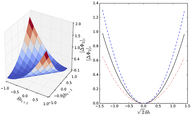
Figure 1. Left: 3d plot of [ΔΦ]_i for the EW case, with ν = 1. Right: projection on the plane δh_i+1 = −δh_i−1. Solid black line: EW case, with ν = 1. Remaining lines: KPZ case (λ = 1) illustrating the breakdown of the “vertical” symmetry δh_i ↔ − δh_i (red dash-dotted line: δh_i = 1; blue dashed line: δh_i = −1).

FIGURE 2

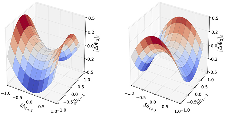
Figure 2. 3d plots of [ΔΦ₃]_i—the third term of the local potential variation for particle i—in the KPZ case, adopting ν = λ = 1. Left: [∇h₀]_i = 1; Right: [∇h₀]_i = −1. Both cases exhibit breakdown of the “horizontal” symmetry δh_i+1 ↔ δh_i−1, but with different signs.

Rather than the quantitative information these figures may provide, some essential aspects—as the local symmetries involved in each case and the dynamical consequences of their breakdown—are worth discussing. We focus on three facts from (7):

1. Since the coefficient of the first-order term is symmetric (similarly to what occurs in the EW case, where this coefficient is proportional to the curvature), the fluctuating local linear field it produces has no consequence whatsoever on the global effect of the potential. A breakdown of this symmetry produces a final global effect in the potential that, if it is uniform, gives rise to a linear potential.

2. When the symmetry under “vertical” flip (namely, changing the sign of δh_i) is broken—as it occurs in the second term of (7), one would expect some asymmetry in the probability density of δh_i.

3. When the symmetry under “horizontal” flip (namely, changing δh_i+1 ↔ δh_i−1) holds, diffusive propagation of fluctuations (and thus z = 2) is expected, as occurs in the EW case. If it is broken by including local ballistic effects—as in the third term of (7)—superdiffusive propagation of fluctuations becomes possible, offering an explanation to the origin of the value z = 3/2 observed in KPZ dynamics.

Note that in the EW case these symmetries hold, while in the KPZ all of them are broken. These facts lend themselves to insightful interpretations that we study in what follows.

Before delving however into the thorough analysis of Φ[h] to which this article is devoted, we find it convenient to introduce a genuine Lyapunov functional for KPZ, to see its pros and cons. The functional

$\begin{array}{ll}{F}\left[h\right]=\frac{\nu }{2}{\displaystyle \int }exp\left[\frac{\lambda }{\nu }h(x,t)\right]{\left[\nabla h(x,t)\right]}^{2}dx,& (8)\end{array}$

of Wio [32], allows the KPZ equation to be written as

$\begin{array}{ll}\frac{\partial }{\partial t}h(x,t)=-\Gamma \left[h\right]\frac{\delta {F}\left[h\right]}{\delta h(x,t)}+\xi (x,t),& (9)\end{array}$

with Γ[h] given by

$\begin{array}{l}\Gamma \left[h\right]=exp\left[-\frac{\lambda }{\nu }h(x,t)\right].\end{array}$

It is straightforward to verify that (i) the Lyapunov property $\dot{{F}}\left[h\right]\le 0$ holds, (ii) the EW free-energy functional is recovered for λ = 0, and (iii) ${\langle {F}\left[h\right]\rangle }_t$ behaves asymptotically as $f(t)exp\left[\frac{\lambda }{\nu }{v}_{\infty }t\right]$, with f(t) far milder than an exponential [2, 3]. Moreover, numerical simulations show that v_∞ ∝ λ, so the asymptotic behavior results ~exp[λ²t].

Since (9) is not of gradient form, ${F}\left[h\right]$ does not provide an intuitive landscape for the stochastic dynamics of h(x, t). So hereafter, we focus on the analysis of Φ[h]. As stated before, its form provokes several thoughts:

2.1. On Normalization

The first-order contribution to the potential in (7) is composed of two terms: one is proportional to the curvature of the initial shape ${\left[{\nabla }^2{h}_0\right]}_i$ and the other (which appears only in the KPZ case) is always positive and given by ${\left[{(\nabla h_0)}^2\right]}_i$. This term breaks the symmetry observed in the EW case and induces a potential which is linear in δh_i. The dynamics is then analog to that of a particle in a constant gravitational field [36]. In this case, the mean position of the particle moves with constant velocity and its fluctuations obey a diffusive behavior. The probability density of the particle keeps evolving (becoming flatter around its mean position) and a stationary solution (and even normalization of this probability) is only possible if there exists an external boundary.

The equilibrium particle distribution in a constant gravitational field would in principle be the stationary limit of the (exact) solution of the Fokker–Planck equation (FPE) associated to the Langevin problem

$\begin{array}{l}\dot{x}=F+\xi (t),\langle \xi (t)\rangle =0,\langle \xi (t)\xi (t\prime )\rangle =D\delta (t-t\prime ),\end{array}$

with the initial condition P(x, t → t₀|x₀, t₀) = δ(x − x₀), if this stationary distribution could be normalized! As known, the physics of this simple problem dictates that there is always a boundary. In fact, the correct interval has a finite limit in the sense of the decreasing potential, thus allowing for normalization [37, 38].

The FPE associated to (1) is [1, 2]

$\begin{array}{l}{\partial }_{t}P[h]={\displaystyle \int \text{d}}x\frac{\delta }{\delta h}\left[-\left(\nu {\nabla }^{2}h+\frac{\lambda }{2}{\left(\nabla h\right)}^2\right)P+D\frac{\delta P}{\delta h}\right]\hfill \\ ={\displaystyle \int \text{d}}x\frac{\delta }{\delta h}\left[\left(\frac{\delta \Phi }{\delta h}\right)P+D\frac{\delta P}{\delta h}\right].\hfill & (10)\end{array}$

In this case, it is not a stationary but an asymptotic solution to (10) what we look for. Forcing the condition ∂_tP[h] = 0 leads to P_as[h] ∝ exp(−Φ[h]/D).

As in the simple analogy before, the pdf in the potential indicated by (7) cannot be normalized except by considering an interval (−∞, h_m].

2.2. On the Statistics

The symmetry under “vertical” flip is broken by the second term of (7) in the KPZ case. When δh_i is positive (see Figure 1), the curvature $2(\nu -\frac{\lambda }{3}\delta h_i)$ of the parabolic potential decreases with respect to the EW value, which means that larger fluctuations are possible of the distance between neighbors. Conversely, when δh_i is negative, the opposite effect occurs. The final global effect will be some asymmetry in the probability distribution of h_i around its mean value, which is in agreement with recent exact results in 1d, where it has been shown that the pdf is not a Gaussian but a Tracy–Widom distribution [16–19]. Recall that since δh_i > ν/λ would produce a negative parabolic potential—meaning local instabilities—the expansion is valid only for short times, such that the potential remains positive.

It is thus worthwhile stressing that the well-known pdf [2, 3]

$\begin{array}{ll}{P}_{stat}\left[h\right]\propto exp\left\{-\frac{\nu }{2D}{\displaystyle {\int }_0^L}{({\partial }_{x}h)}^{2}dx\right\},& (11)\end{array}$

makes sense only for a finite 1d system with periodic boundary conditions and for times larger than t ~ L^z, the saturation one.

2.3. Potential Landscape's Long Memory

The second term in (5), namely

$\begin{array}{ll}-\frac{\lambda }{2}{\displaystyle \int \text{d}}x{\displaystyle {\int }_{h_0(x,0)}^{h(x,t)}\text{d}\psi {\left(\nabla \psi \right)}^2,}& (12)\end{array}$

is not a functional integral of the form ∫∏_x dψ(x) [39], but a kind of “grand mean” of (∇h)². For a suitably small time τ, the integral over ψ at fixed x can be evaluated by resort to the Mean Value Theorem, yielding

$\begin{array}{ll}{\displaystyle {\int }_{h_0(x,0)}^{h(x,\tau )}\text{d}}\psi {\left(\nabla \psi \right)}^2\approx \left[h\left(x,\tau \right)-h\left(x,0\right)\right]{\left[\nabla \tilde{h}(x)\right]}^2,& (13\text{a})\end{array}$

where $\tilde{h}(\text{x})$ is some intermediate value between h(x, τ) and h(x, 0). For finite time t, a discretization with step τ and index μ yields

$\begin{array}{l}{\displaystyle {\int }_{h_0(x,0)}^{h(x,t)}\text{d}}\psi {\left(\nabla \psi \right)}^2\approx {\displaystyle \sum _{\mu =0}^{M-1}\tau }\frac{h_{\mu +1}(x)-h_{\mu }(x)}{\tau }{\left[\nabla {\tilde{h}}_{\mu }(x)\right]}^2\\ \approx {\displaystyle {\int }_0^t\text{d}}s\dot{h}(x,s){\left[\nabla h(x,s)\right]}^2,& (13\text{b})\end{array}$

with ${\tilde{h}}_{\mu }(\text{x})$ intermediate between h_μ(x) and h_μ+1(x), and $\dot{h}$(x, s): = lim_τ→0[h_μ+1(x) − h_μ(x)]/τ. This allows us to write the potential in the form

$\begin{array}{ll}\Phi [h]={\displaystyle \int \text{d}}x\left\{\frac{\nu }{2}{\left(\nabla h\right)}^2-\frac{\lambda }{2}{\displaystyle {\int }_0^t\text{d}}s\dot{h}(x,s){\left[\nabla h(x,s)\right]}^2\right\},& (14)\end{array}$

which highlights the fact that even though the field h(x, t) obeys a Fokker–Planck equation (thus it is Markovian, albeit without stationary regime), it evolves at every time in an adaptive potential landscape, which itself evolves according to the whole history of h(x, t) and has thus a very long (“infinite”) memory. The already mentioned dependence of the asymptotic statistics on the dynamics of the substrate might probably be traced back to this fact [16–20].

3. Numerical Results for Φ[h]

Spectral methods pay back the overhead of Fourier transforming h(x) forth and back every time t, with a discrete approximation of ∇h of the order of the system's size. They have proved to be more stable and reliable than pure real-space finite-differences schemes in the integration of some non-linear growth equations [40–42]. Using a spectral method to integrate (1), we have analyzed the time behavior of 〈Φ[h]〉_t (the average of Φ over noise realizations, at time t) as given by (14).

Figure 3 displays the time dependence of the NEP's average over 100 samples, for systems in 1d (size 1,024), 2d (size 128²), and 3d (size 64³), and several values of λ. For any λ > 0 there is a maximum, where the non-linear (KPZ) term overcomes the linear (EW) one. Only for λ = 0 (corresponding to EW) is there true saturation. The λ = 0.01 case shown here (visually resembling a saturation behavior) attains its maximum outside the plotted range.

FIGURE 3

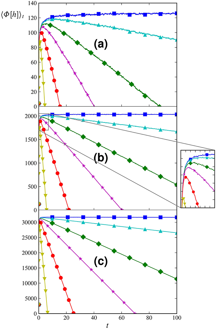
Figure 3. Time behavior of Φ[h], averaged over 100 samples, in (A) 1d (size 1024), (B) 2d (size 128²), and (C) 3d (size 64³). The symbols (denoting a subset of the simulation points) indicate the values adopted for λ in each curve. ■ : λ = 0.01, ▴ : λ = 0.10, ◇ : λ = 0.20, ⋆ : λ = 0.30, • : λ = 0.50, ▾ : λ = 1.00. Inset: Detail showing the existence of maxima in 2d for any λ > 0 (the same occurs in 1d and 3d).

Figure 4—as well as (16) and (17) below—shows that past this maximum, 〈Φ[h(t)]〉_t ~ A − Bt with B ~ λ². This result shows that—due to the correlations and in an effective way—the NEP behaves as having only a linear dependence on h (just as in the toy model discussed before [37, 38]).

FIGURE 4

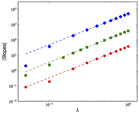
Figure 4. Mean λ-dependence over 100 samples of the NEP's asymptotic slope. Here, the symbols denote the substrate's dimensionality: ◇ 1d (size 1024), ■ 2d (size 128²), and • 3d (size 64³). The dashed lines (besides guiding the eye) are best fits with a λ^b (b = 2.01 in d = 1 and 2, and b = 2.03 in 3d).

Figure 5 shows the dependence on λ of the time t_xovr at which the maximum occurs, i.e., at which the non-linear (KPZ) contribution overcomes the linear (EW) one, making it a proxy of the EW-to-KPZ crossover time [43–45]. Although roughly compatible with a $t_{xovr}~{\lambda }^{-\alpha }$ law (α = 3 in Guo et al. [43] and α = 4 in Forrest and Toral, [44] for d = 1) and in agreement with the results of previous studies exploiting the time behavior of the stochastic action [46, 47], this dependence becomes milder as d increases.

FIGURE 5

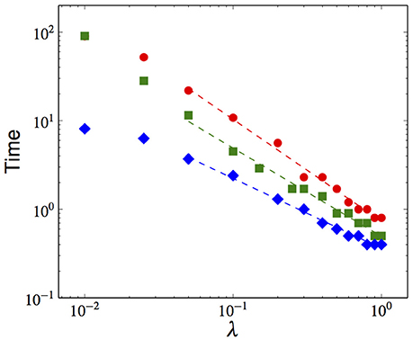
Figure 5. Mean λ-dependence over 100 samples of the time of occurrence of the NEP's maximum, in •: 1d (size 1024), ■: 2d (size 128²), and ◇: 3d (size 64³). Dashed lines: best fits with a λ^−b yield b = 1.14 in 1d, b = 0.98 in 2d, and b = 0.79 in 3d.

3.1. External Field

By including an external driving force F, it is possible to capture some new aspects of the dynamics. Equation (5) now reads

$\Phi [h]={\displaystyle \int \text{d}}x\left[\frac{\nu }{2}{(\nabla h)}^2-\frac{\lambda }{2}{\displaystyle {\int }_{h_0(x,0)}^{h(x,t)}\text{d}}\psi {(\nabla \psi )}^2-Fh(x,t)\right].$

Figure 6 shows (on a much longer timescale than in Figure 3, so that the already discussed initial rise due to the EW term cannot be appreciated) the NEP's time behavior for both positive and negative values of F. The F > 0 case brings no novelty; but when negative enough forces are applied, a reversion is observed of the NEP's time behavior, corresponding to a reversion of the front motion 〈h〉 and supporting the analogy to an activation-like behavior (which could be guessed from the cubic-like form of the NEP). As already stated however, this behavior is not of the exponential (Kramers-like) form. Moreover the abovementioned diffusive instability, now written as

$\begin{array}{ll}\Phi [h]={\displaystyle \int \text{d}}x\left[\left(\frac{\nu }{2}-\frac{\lambda \delta h}{6}\right){\left(\nabla \delta h\right)}^2-F\delta h\right],& (15)\end{array}$

limits its validity to a range of F. If F < 0, the evolution toward negative values of δh(x, t) proceeds mainly along the almost zero-measure subset of directions where ∇δh(x, t) = 0. However, as soon as—due to the presence of noise—δh(x, t) slightly depart from those directions, the effect of the NEP is such that it will drive the system in the opposite direction! At any rate, this will only happen for F larger than some threshold value. Thus, for F = 0, the time behaviors of 〈Φ[h]〉 and 〈h〉 are correlated, even though the dispersion of the NEP [48] and that of the front differ (the former continuously increases with time, while the latter saturates for t ≥ L^z). These aspects will be fully clarified in the next section. For the time being let us remind that in the EW case and without external force, 〈h〉 = 0. If a force F is applied, the EW NEP acquires the form

${\Phi }_{\text{EW}}[h(x,t)]=\frac{\nu }{2}{\displaystyle \int \text{d}}x\left\{{\left[\nabla h\left(x,t\right)\right]}^2-Fh(x,t)\right\}.$

FIGURE 6

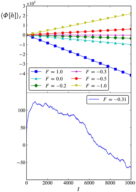
Figure 6. NEP's long-time behavior in 1d (λ = 1), from 100 samples of size 256. Upper frame: For F < −0.3, 〈Φ[h]〉 increases with time in the observation interval. Lower frame: detail showing that for F just slightly lower than −0.3, 〈Φ[h]〉 first increases with time (on a much longer timescale than the initial rise due to the EW term) and then begins to decrease, supporting the hypothesis of an activation-like behavior.

When the linear term largely exceeds the quadratic one, the EW equation becomes $\dot{h}$ = νF, so 〈h〉 → νFt. This effect seems to indicate that including an external force reinforces the statistical weight of those directions such that ∇δh(x, t) = 0, which for F = 0 have (almost) zero measure. As a matter of fact, neither the inclusion of the external force F nor the effects shown in Figure 6 change the scaling behavior.

4. Some Asymptotic Results

As known in the EW case [2–4] and shown in Figure 3, the average 〈 ∫ dx(∇h)²〉 over noise realizations saturates to a constant C₀ at long times. Using in (15) the discrete expression for Φ[h]—namely (12), with the approximation in (13b)—we can write

$\begin{array}{l}\langle \Phi [h]\rangle =\nu C_0-\frac{\lambda }{2}\langle {\displaystyle \int \text{d}}x{\displaystyle \int \text{d}}\psi {\left(\nabla \psi \right)}^2\rangle -F\langle h\rangle \hfill \\ \approx \nu C_0-\frac{\lambda }{2}\langle {\displaystyle \sum _{\text{space}}{\displaystyle \sum _{\text{time}}\delta }}h{\left(\nabla h\right)}^2\rangle -F\langle h\rangle .\hfill & (16)\end{array}$

In the discrete representation, (3) implies δh ~ v_∞τ at long times, where τ corresponds to δt and v_∞ is the asymptotic front velocity. Inserting this expression into the previous one and replacing 〈 ∫ dx(∇h)²〉 by its bound C₀, we get

$\begin{array}{ll}\langle \Phi \left[h\right]\rangle =\frac{\nu }{2}{C}_0-(\frac{\lambda }{2}{C}_0+F)v_{\infty }t.& (17)\end{array}$

This result, valid in any dimensionality, completely agrees with the numerical ones presented above. In particular, 〈Φ[h]〉 will decrease at long times only if λC₀ + F ≥ 0. If λC₀ + F < 0, 〈Φ[h]〉 will increase asymptotically, as shown in Figure 6. In addition, it is well-known that v_∞ ∝ λ [3]. Hence (particularly in the F = 0 case) we find the λ² dependence for the slope of 〈Φ[h]〉 vs. t, as obtained in simulations.

We close this section by looking at the asymptotic behavior from another point of view. Here we restrict to d = 1, the continuum representation, and the F = 0 case. As already indicated, the statistics of the stochastic variable χ in (3), is of paramount importance [16, 17]. In addition to the forms of Φ[h] given by (5) and (14), we can also obtain an expression for $\dot{\Phi }\left[h\right]$ as

$\begin{array}{ll}\dot{\Phi }\left[h\right]=-{\displaystyle \int }dx\left[\nu {\partial }_x^{2}h+\frac{\lambda }{2}{({\partial }_{x}h)}^2\right]\dot{h}.& (18)\end{array}$

We have the following relations

$\begin{array}{l}{\partial }_{x}h={\left(\Gamma t\right)}^{1/3}{\partial }_{x^{\prime }}\chi \left(\frac{\text{d}{x}^{\prime }}{\text{d}x}\right)~\frac{A}{2}{\left(\Gamma t\right)}^{1/3}{\left(\Gamma t\right)}^{-2/3}{\chi }^{\prime }\\ ~\frac{A}{2}{\left(\Gamma t\right)}^{-1/3}{\chi }^{\prime },& (19)\end{array}$

with ${\chi }^{\prime }:={\partial }_x\chi$. The time derivative of (3) is

$\begin{array}{ll}\dot{h}~v_{\infty }+\frac{\Gamma }{3}{\left(\Gamma t\right)}^{-2/3}\chi -\frac{\Gamma }{3}Ax{\left(\Gamma t\right)}^{-4/3}{\chi }^{\prime }~v_{\infty },& (20)\end{array}$

as the 2nd and 3rd terms decay very fast. On the other hand,

${\left({\partial }_{x}h\right)}^2~\frac{A^2}{4}{\left(\Gamma t\right)}^{-2/3}{\left({\chi }^{\prime }\right)}^2,{\partial }_x^{2}h~\frac{A^2}{4}{\left(\Gamma t\right)}^{-1}{\chi }^{″}.$

Exploiting these relations we obtain

$\begin{array}{ll}\dot{\Phi }\left[h\right]~-{\displaystyle \int }d{x}^{\prime }\frac{A}{2}\left[\nu {\chi }^{″}+\frac{\lambda }{2}{({\chi }^{\prime })}^2\right]v_{\infty }.& (21)\end{array}$

If we look at long times, where the non-linear contribution dominates, we have

$\begin{array}{ll}\dot{\Phi }\left[h\right]~-{\displaystyle \int }d{x}^{\prime }\frac{A\lambda }{4}{({\chi }^{\prime })}^2{v}_{\infty }.& (22)\end{array}$

Since v_∞ ∝ λ, we get right away the expected result: the constant goes as λ².

We now show why 〈Φ[h]〉 and 〈h〉 are correlated. At long times, when $\langle \int \text{d}\text{x}{(\nabla \delta h)}^2\rangle \to C_0$ and 〈h〉 → v_∞t, (13b)—now in terms of δh—“factorizes” out and thus ${\delta }^3\Phi \left[h(\text{x},t)\right]\to -\lambda C_0\langle h\rangle$. Hence the second term in (5)—which already dominates over the first one—behaves in the same way as the term in EW corresponding to an external force:

$\begin{array}{l}-\frac{\lambda }{2}{\displaystyle \int \text{d}}x{\displaystyle {\int }_{h_0(x,0)}^{h(x,t)}\text{d}}\psi {\left(\nabla \psi \right)}^2\to -\frac{\lambda }{2}{\displaystyle \int \text{d}}x\delta h(x,t){\left[\nabla \delta h(x,t)\right]}^2\\ \approx -\frac{\lambda }{2}{C}_0\langle h\rangle .\end{array}$

5. Conclusions

For any substrate dimensionality d, the KPZ equation can be expressed as a gradient flow by means of the functional Φ[h(x, t)] in (5). This is a state functional, i.e., it depends explicitly only on h(x, t). However, evaluating Φ[h] for a given field configuration h(x, t) requires integrating over its whole story, with initial condition h₀(x). So Φ[h] carries information on the whole growth story. If (5) is discretized according to ${(\nabla h)}^2\to \frac{1}{2}\left[{(h_{i+1}-h_i)}^2+{(h_{i-1}-h_i)}^2\right]$ [11, 12], a cubic polynomial in the {h_i}—containing $h_i^3$ terms—is obtained.

Expansion (6) provides an “instantaneous landscape” of Φ[h(x, t)]. Even using ${(\nabla h)}^2\to {(h_{i+1}-h_{i-1})}^2$, its discretization also yields a cubic polynomial (in the {δh_i}) but now the absence of $\delta h_i^3$ terms enables a clearer understanding of “horizontal” and “vertical” symmetry breakdowns when λ ≠ 0—which may in turn be related to the asymmetry of the Tracy–Widom distribution—and brings an explanation to the shift in the dynamical exponent z (a change from diffusive to superdiffusive behavior).

Even though Φ[h] fulfills the Lyapunov property, its functional form is for short times that of a cubic polynomial, and is thus unbounded below. The KPZ equation turns out to be a high-dimensional (non Kramers) escape-like problem, and its asymptotic pdf cannot be normalized on the whole h–space (except for fixed and normalized forms of h₀). We have moreover provided a bridge between the observed asymptotic Tracy–Widom statistics, and the behavior of Φ (which as argued, provides an instantaneous landscape for the stochastic dynamics).

Given an ensemble of stories h(x, t), one can attempt to calculate the time dependence of the lower moments of Φ[h]. Our focus in this work is on 〈Φ[h]〉_t, the average of Φ[h] over noise realizations at time t. We have shown both numerically (Figures 3, 4) and analytically in (17) that in the absence of external forcing (F = 0), 〈Φ[h]〉_t → A − Bt as t → ∞ (in fact, surprisingly soon!), with B ~ λ². We have moreover traced back the origin of this asymptotic linear dependence on t to two known effects: (a) 〈h〉 → v_∞t, (b) $\langle \int \text{d}\text{x}{(\nabla h)}^2\rangle \to C_0$, which lead to factorization of the “KPZ term” in 〈Φ[h]〉_t.

The time t_max at which 〈Φ[h]〉_t goes through a maximum, can be regarded as an estimation of the crossover time t_xovr from the EW regime to the KPZ one. We have found that $t_{max}~{\lambda }^{-1}$, in agreement with previous results obtained by exploiting the time behavior of the stochastic action [46, 47].

Other issues worth remarking are that—because of the abovementioned linear dependence of 〈Φ[h]〉_t on t—the behaviors of 〈Φ[h]〉_t and 〈h〉 are correlated, and that (both with and without external forcing) the NEP's time behavior indicates a (non Kramers) activation-like phenomenon. In a forthcoming work [48] we undertake a thorough analysis of the time behavior of the first few higher moments of Φ[h], namely the NEP's dispersion σ(t), skewness γ₁(t) and kurtosis K(t). An interesting point (left to further work) would be to “interpret” the aging phenomenon [49, 50] from the NEP perspective.

We have discussed some strengths of a novel tool for describing the KPZ dynamics, the NEP approach. This innovative framework is expected to contribute answering questions that remain open by today, and handling the KPZ problem from still another perspective [13, 36].

Author Contributions

All authors listed, have made substantial, direct and intellectual contribution to the work, and approved it for publication.

Conflict of Interest Statement

The authors declare that the research was conducted in the absence of any commercial or financial relationships that could be construed as a potential conflict of interest.

Acknowledgments

Support by MINECO (Spain), under project No. FIS2014-59462-P, is acknowledged by HW, MR, and RG; support by CONICET, UNMdP and UNC (Argentina), by RD and JR. The authors thank J.M. López, R. Toral, C. Escudero, P. Colet and E. Hernández-García for fruitful discussions.

Footnotes

1. ^We deliberately leave aside KIR models exhibiting diverse kinds of anomalous scaling [6, 7].

2. ^Both discretizations of the KPZ equation and microscopic KIR models generically break GI. But even in the few cases explicitly built to preserve GI, the periodic boundary conditions (PBC) customarily adopted in numerical simulations explicitly break down tilting invariance (note in passing that spectral methods rely more than any other on PBC). A recent result supporting this is that cellular automata models for etching have been shown to obey (1) up to d = 6 [13].

3. ^The Gaussian orthogonal ensemble (GOE) if the substrate is static, the Gaussian unitary (GUE) one if it evolves [21, 22].

References

1. Kardar M, Parisi G, Zhang YC. Dynamic scaling of growing interfaces. Phys Rev Lett. (1986) 56:889–92. doi: 10.1103/PhysRevLett.56.889

PubMed Abstract | CrossRef Full Text | Google Scholar

2. Halpin-Healy T, Zhang YC. Kinetic roughening phenomena, stochastic growth, directed polymers and all that: aspects of multidisciplinary statistical mechanics. Phys Rep. (1995) 254:215–414. doi: 10.1016/0370-1573(94)00087-J

CrossRef Full Text | Google Scholar

3. Barabási AL, Stanley HE. Fractal Concepts in Surface Growth. Cambridge, UK: Cambridge University Press (1995).

4. Krug J. Origins of scale invariance in growth processes. Adv Phys. (1997) 46:139–282. doi: 10.1080/00018739700101498

CrossRef Full Text | Google Scholar

5. Lesne A, Laguës M. Scale Invariance: From Phase Transitions to Turbulence. Berlin: Springer (2012).

Google Scholar

6. Ramasco JJ, López JM, Rodríguez MA. Generic dynamic scaling in kinetic roughening. Phys Rev Lett. (2000) 84:2199–202. doi: 10.1103/PhysRevLett.84.2199

PubMed Abstract | CrossRef Full Text | Google Scholar

7. Wio HS, Deza RR, López JM. An Introduction to Stochastic Processes and Nonequilibrium Statistical Physics. Singapore: World Scientific (2012).

Google Scholar

8. Holden H, Lindstrøm T, Øksendal B, Ubøe J, Zhang TS. The Burgers equation with noisy force and the stochastic heat equation. Comm Partial Diff Eq. (1994) 19:119–41. doi: 10.1080/03605309408821011

CrossRef Full Text | Google Scholar

9. Fogedby H. Morphology and scaling in the noisy Burgers equation: soliton approach to the strong coupling fixed point. Phys Rev Lett. (1998) 80:1126–9. doi: 10.1103/PhysRevLett.80.1126

CrossRef Full Text | Google Scholar

10. Fogedby H. Canonical phase-space approach to the noisy Burgers equation. Phys Rev E (1999) 60:4950–3. doi: 10.1103/PhysRevE.60.4950

PubMed Abstract | CrossRef Full Text | Google Scholar

11. Wio HS, Revelli JA, Deza RR, Escudero C, de La Lama MS. KPZ equation: galilean-invariance violation, consistency, and fluctuation–dissipation issues in real-space discretization. Europhys Lett. (2010) 89:40008. doi: 10.1209/0295-5075/89/40008

PubMed Abstract | CrossRef Full Text | Google Scholar

12. Wio HS, Revelli JA, Deza RR, Escudero C, de La Lama MS. Discretization-related issues in the Kardar–Parisi–Zhang equation: consistency, Galilean-invariance violation, and fluctuation–dissipation relation. Phys Rev E. (2010) 81:066706. doi: 10.1103/PhysRevE.81.066706

PubMed Abstract | CrossRef Full Text | Google Scholar

13. Rodrigues EA, Mello BA, Oliveira FA. Growth exponents of the etching model in high dimensions. J Phys A. (2015) 48:035001. doi: 10.1088/1751-8113/48/3/035001

CrossRef Full Text | Google Scholar

14. Kapral R, Livi R, Oppo GL, Politi A. Dynamics of complex interfaces. Phys Rev E. (1994) 49:2009–22. doi: 10.1103/PhysRevE.49.2009

PubMed Abstract | CrossRef Full Text | Google Scholar

15. Xu Z, Han H, Wu X. Numerical method for the deterministic Kardar–Parisi–Zhang equation in unbounded domains. Comm Comput Phys. (2006) 1:479–93.

Google Scholar

16. Prähofer M, Spohn H. Statistical self-similarity of one-dimensional growth processes. Physica A. (2000) 279:342–52. doi: 10.1016/S0378-4371(99)00517-8

CrossRef Full Text

17. Prähofer M, Spohn H. Universal distributions for growth processes in 1+1 dimensions and random matrices. Phys Rev Lett. (2000) 84:4882–5. doi: 10.1103/PhysRevLett.84.4882

PubMed Abstract | CrossRef Full Text

18. Sasamoto T, Spohn H. One-dimensional Kardar–Parisi–Zhang equation: an exact solution and its universality. Phys Rev Lett. (2010) 104:230602. doi: 10.1103/PhysRevLett.104.230602

PubMed Abstract | CrossRef Full Text | Google Scholar

19. Calabrese P, Le Doussal P. Exact solution for the Kardar–Parisi–Zhang equation with flat initial conditions. Phys Rev Lett. (2011) 106:250603. doi: 10.1103/PhysRevLett.106.250603

PubMed Abstract | CrossRef Full Text | Google Scholar

20. Takeuchi KA. Crossover from growing to stationary interfaces in the Kardar–Parisi–Zhang class. Phys Rev Lett. (2013) 110:210604. doi: 10.1103/PhysRevLett.110.210604

PubMed Abstract | CrossRef Full Text | Google Scholar

21. Halpin-Healy T, Takeuchi KA. A KPZ cocktail—shaken, not stirred…Toasting 30 years of kinetically roughened surfaces. J Stat Phys. (2015) 160:794–814. doi: 10.1007/s10955-015-1282-1

PubMed Abstract | CrossRef Full Text

22. Carrasco ISS, Takeuchi KA, Ferreira SC, Oliveira TJ. Interface fluctuations for deposition on enlarging flat substrates. New J Phys. (2014) 16:123057. doi: 10.1088/1367-2630/16/12/123057

CrossRef Full Text | Google Scholar

23. Baik J, Rains EM. Limiting distributions for a polynuclear growth model with external sources. J Stat Phys. (2000) 100:523–41. doi: 10.1023/A:1018615306992

CrossRef Full Text | Google Scholar

24. Corwin I. The Kardar–Parisi–Zhang equation and universality class. Rand Matrices Theory Appl. (2012) 1:1130001. doi: 10.1142/S2010326311300014

PubMed Abstract | CrossRef Full Text | Google Scholar

25. Imamura T, Sasamoto T. Exact solution for the stationary Kardar–Parisi–Zhang equation. Phys Rev Lett. (2012) 108:190603. doi: 10.1103/PhysRevLett.108.190603

PubMed Abstract | CrossRef Full Text | Google Scholar

26. Hairer M. Solving the KPZ equation. Ann Math. (2013) 178:559–664. doi: 10.4007/annals.2013.178.2.4

CrossRef Full Text | Google Scholar

27. Takeuchi KA, Sano M. Universal fluctuations of growing interfaces: evidence in turbulent liquid crystals. Phys Rev Lett. (2010) 104:230601. doi: 10.1103/PhysRevLett.104.230601

PubMed Abstract | CrossRef Full Text | Google Scholar

28. Takeuchi KA, Sano M, Sasamoto T, Spohn T. Growing interfaces uncover universal fluctuations behind scale invariance. Sci Rep (Nature). (2011) 1:34. doi: 10.1038/srep00034

PubMed Abstract | CrossRef Full Text | Google Scholar

29. Takeuchi KA, Sano M. Evidence for geometry-dependent universal fluctuations of the Kardar–Parisi–Zhang interfaces in liquid-crystal turbulence. J Stat Phys. (2012) 147:853–90. doi: 10.1007/s10955-012-0503-0

CrossRef Full Text | Google Scholar

30. Halpin-Healy T. (2+1)-dimensional directed polymer in a random medium: scaling phenomena and universal distributions. Phys Rev Lett. (2012) 109:170602. doi: 10.1103/PhysRevLett.109.170602

PubMed Abstract | CrossRef Full Text | Google Scholar

31. Halpin-Healy T. Extremal paths, the stochastic heat equation, and the three-dimensional Kardar–Parisi–Zhang universality class. Phys Rev E (2013) 88:042118. doi: 10.1103/PhysRevE.88.042118

PubMed Abstract | CrossRef Full Text | Google Scholar

32. Wio HS. Variational formulation for the KPZ and related kinetic equations. Int J Bif Chaos. (2009) 19:2813–21. doi: 10.1142/S0218127409024505

CrossRef Full Text | Google Scholar

33. Wio HS, Escudero C, Revelli JA, Deza RR, de La Lama MS. Recent developments on the Kardar–Parisi–Zhang surface-growth equation. Phil Trans R Soc A. (2011) 369:396–411. doi: 10.1098/rsta.2010.0259

PubMed Abstract | CrossRef Full Text | Google Scholar

34. Wio HS, Deza RR, Escudero C, Revelli JA. Invited review: KPZ. Recent developments via a variational formulation. Papers Phys. (2013) 5:050010. doi: 10.1098/rsta.2010.0259

CrossRef Full Text | Google Scholar

35. Graham R. “Weak noise limit and nonequilibrium potentials of dissipative dynamical systems,” In: Tirapegui E, Villarroel D, editors. Instabilities and Nonequilibrium Structures. Dordrecht: D. Reidel (1987). p. 271–90.

36. Saka H, Bengtson RD, Reichl LE. Relaxation of Brownian particles in a gravitational field. Am J Phys. (2009) 77:240–3. doi: 10.1119/1.3039029

PubMed Abstract | CrossRef Full Text | Google Scholar

37. van Kampen NG. Stochastic Processes in Physics and Chemistry. Amsterdam: North-Holland (1990).

Google Scholar

38. Gardiner CW. Handbook of Stochastic Methods for Physics, Chemistry and the Natural Sciences. Berlin: Springer (2004).

Google Scholar

39. Langouche F, Roekaerts D, Tirapegui E. Functional Integration and Semiclassical Expansions. Dordrecht: Reidel (1982).

Google Scholar

40. Gallego R, Castro M, López JM. Pseudospectral versus finite-difference schemes in the numerical integration of stochastic models of surface growth. Phys Rev E (2007) 76:051121. doi: 10.1103/PhysRevE.76.051121

PubMed Abstract | CrossRef Full Text | Google Scholar

41. Giada L, Giacometti A, Rossi M. Pseudospectral method for the Kardar–Parisi–Zhang equation. Phys Rev E. (2002) 65:036134. doi: 10.1103/PhysRevE.65.036134

PubMed Abstract | CrossRef Full Text | Google Scholar

42. Gallego R. Predictor–corrector pseudospectral methods for stochastic partial differential equations with additive white noise. Appl Math Comp. (2011) 218:3905–17. doi: 10.1016/j.amc.2011.09.038

CrossRef Full Text | Google Scholar

43. Guo H, Grossmann B, Grant M. Crossover scaling in the dynamics of driven systems. Phys Rev A. (1990) 41:7082–5. doi: 10.1103/PhysRevA.41.7082

PubMed Abstract | CrossRef Full Text | Google Scholar

44. Forrest BM, Toral R. Crossover and finite-size effects in the (1+1)-dimensional Kardar–Parisi–Zhang equation. J Stat Phys. (1993) 70:703–20. doi: 10.1007/BF01053591

CrossRef Full Text | Google Scholar

45. Oliveira TJ, Dechoum K, Redinz JA, Aarão Reis FDA. Universal and nonuniversal features in the crossover from linear to nonlinear interface growth.Phys Rev E. (2006) 74:011604. doi: 10.1103/PhysRevE.74.011604

PubMed Abstract | CrossRef Full Text | Google Scholar

46. Wio HS, Deza RR, Revelli JA, Escudero C. A novel approach to the KPZ dynamics. Acta Phys Polon B. (2013) 44:889–98. doi: 10.5506/APhysPolB.44.889

PubMed Abstract | CrossRef Full Text | Google Scholar

47. Wio HS, Revelli JA, Gallego R, Rodríguez MA, Deza RR. Estimation of the crossover time in arbitrary dimensions for the KPZ equation, through the analysis of its stochastic action. (2016).

48. Wio HS, Gallego R, Rodríguez MA, Alés A, Deza RR, Revelli JA. Generating functional for the KPZ equation in arbitrary dimensions: time evolution of its higher cumulants. (2016).

49. Bustingorry S. Aging dynamics of non-linear elastic interfaces: the Kardar–Parisi–Zhang equation. J Stat Mech Theory Exp. (2007) 10:P10002. doi: 10.1088/1742-5468/2007/10/P10002

CrossRef Full Text | Google Scholar

50. Henkel M, Noh JD, Pleimling M. Phenomenology of aging in the Kardar–Parisi–Zhang equation. Phys Rev E. (2012) 85:030102(R). doi: 10.1103/PhysRevE.85.030102

PubMed Abstract | CrossRef Full Text