Augmentation of 3D Holographic Image Graticule With Conventional Microscopy

In this paper, we report an implementation of a computer-generated holographic projection technique to display a holographic scene like a measuring graticule around the magnified sample image in a reflected bright-field microscopy. The implemented system acts as a gauging tool for lateral and longitudinal measurements of a sample that is being observed under a microscope through the assistance of a holographic measuring graticule. Numerical and experimental verifications have been performed, demonstrating the successful augmentation of a holographic projection system as a measuring tool with a conventional bright-field microscopic system.

Introduction

Conventional optical microscopes have been around for many years and are extensively used in biological and medical science applications as well as in the electronics industry. An optical microscope has a simple optical geometry comprising an infinite-corrected objective lens and a tube lens to form a real, inverted, and magnified image of the sample at the back focal plane. This image is further magnified by an ocular lens or eyepiece responsible for presenting an upright magnified virtual image to the user’s eye. Bright-field microscopy is one of the simplest optical microscopy in which a sample is illuminated, and the contrast is generated from the reflected light (McArthur, 1945; McArthur, 1958). For the measurement purpose of the sample on the microscopic stage, the optical microscopes are usually equipped with a reticle or graticule. A graticule is a two-dimensional (2D) disk that is present in an ocular lens to measure the lateral distances of samples on the microscope stage at the focal plane. Due to its 2D structure, it is not suitable for the depth estimation of a magnified sample on a longitudinal axis. Moreover, the 2D graticule needs to be calibrated whenever there is a need to change an objective lens. Usually, calibration can be done by adjusting the 2D graticule to lie side by side with a microscopic scale on the sample stage. From that, a conversion factor is calculated and used in the measurement of lateral distances of a magnified sample. In this paper, we propose implementing an augmentation of a three-dimensional (3D) holographic projection display with a conventional bright-field microscopic system for the lateral and longitudinal measurement of a magnified sample. With a conventional 2D graticule, only latitude measurements in a 2D plane are possible. Also, calibration has to be done with the micrometer scale on the stage sample. This needs to be done every time an objective lens has changed. A 2D graticule needs to be replaced with the appropriate one for different measurement purposes. With the proposed configuration, only complex field information needs to be synthesized without an actual replacement of a physical disk-shaped graticule. Also, longitudinal measurements are possible with the proposed method, which helps in the depth estimation or thickness measurement of an object sample. The proposed augmentation of the 3D holographic projection graticule can be applied to other types of microscopy, e.g., reflected/transmitted brightfield or darkfield microscopic techniques.

For the generation of holographic contents in 3D displays and holographic projectors, computer generated hologram (CGH) plays a vital role. The 3D data of objects in CGH generation can be represented in various forms, such as point cloud (Lucente, 1933), light rays (Wakunami and Yamaguchi, 2011), depth layers (Zhao et al., 2015), and triangular meshes (Kim et al., 2008; Ji et al., 2016). The synthesized complex field is then encoded to either amplitude-only or phase-only CGH before being uploaded to the spatial light modulator (SLM) in the reconstruction process. A peculiar advantage of the CGH over 2D images is the conservation of depth information. Among various CGH techniques, the lensless holographic projection technique is attractive for its robustness and compact geometry, eliminating lens aberration and producing high contrast images (Buckley et al., 2011; Makowski et al., 2016a).

In this paper, we augment a 3D holographic graticule for the microscopic measurement of a magnified sample image around the intermediate image plane, i.e., the back focal plane of the tube lens. For the calculation of the complex field at the SLM plane, we consider a lensless holographic projection geometry that is capable of generating zoomable images with the use of the scaled and shifted Fresnel diffraction (Muffoletto et al., 2007; Shimobaba et al., 2012; Shimobaba et al., 2013; Zhang et al., 2019) algorithm. The scaled and shifted Fresnel diffraction is a fast Fourier transform (FFT) based diffraction calculation considering different sampling rates in the SLM and target image plane. We calculate a 2D holographic image graticule with a large depth of focus (DOF) for the lateral measurement by applying a slowly varying spherical phase distribution to the target image plane (Makowski et al., 2016b). We compute a 3D holographic layer-based graticule around an intermediate image plane for the longitudinal measurement, with each layer having a shallow DOF. Taking advantage of the capacity of superposition of the hologram, we can combine the two complex amplitude distributions before final encoding to a phase-only CGH at the reconstruction step. In the following sections, the principle and configuration of the proposed system is explained. The numerical simulation and optical experiment results are also presented for verification.

Brief Introduction to Reflected Bright-Field Microscopy

Reflected bright-field microscopy is frequently used in industrial applications, especially in the semiconductor area with a metallic sample, integrated circuits, or surface of ceramics. Bright-field or dark-field illumination technique represents dark and bright images against bright and dark backgrounds, respectively (McArthur, 1945; McArthur, 1958). Each illumination technique has its merits and demerits depending on the observed sample. Our experiment considered the bright-field reflected-light microscopy with Kohler’s illumination to eliminate incoherent light-emitting-diode (LED) source image in the intermediate image plane. Figure 1 shows the schematic of a bright-field reflected-light microscope with light ray representation. Orange rays show the focus plane of the light source image, and green rays show the focus plane of the magnified sample image. The magnified sample image is focused in the intermediate image plane or user’s retina, and the source image is highly defocused for better visual acuity. The sample object is placed in the front focal plane of an infinity-corrected objective lens to sharply focus the magnified image in the intermediate image plane with a designed tube lens. The objective lens has two functions: it acts as a condenser lens to focus light on the object sample and to form an image by collecting the reflected light. The parallel green rays from the objective lens to the tube lens constitute a variable distance and can be used to add optical components to the system, such as optical filters and beam splitters. The aperture diaphragm changes the illumination cone to project into the objective lens, which controls the contrast of the sample image. The field diaphragm controls the width of the bundle of light rays reaching the condenser or the objective lens in this reflected microscope case. The overall magnification of the system is calculated by multiplying the objective magnification with the ocular or eyepiece magnification. If a CCD sensor is used to capture the real magnified, inverted sample image in the intermediate image plane, the only magnification to be considered is that of the objective lens. The objective lens has different lateral and longitudinal magnifications like other optical imaging systems. Lateral magnification is defined as the ratio of image height to the object height and is given by the lens manufacturer as “×5”, “×10” means the lens magnifies the object to look five or ten times larger than the actual size. The longitudinal magnification is defined as the square of lateral magnification along an optical axis. So, with a ×10 objective lens, the longitudinal magnification for an object sample would be ×100.

FIGURE 1

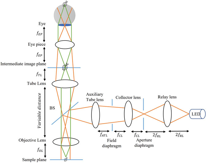
FIGURE 1. Schematic of a reflected bright-field microscope.

Calculation of a Complex Hologram

For the generation of complex amplitude distribution at the SLM plane, we consider the lensless holographic projection technique, as shown in Figure 2. It has a compact geometry with a single SLM and a projection screen at a propagation distance $\mathit{z}$. Note that the intermediate image plane in Figure 1 and the image plane in Figure 2 are overlapping image planes for a magnified sample image and a holographic image, respectively. They are given different names to avoid misunderstanding while discussing their optical geometries individually. At the reconstruction image plane, $\mathit{I}(\mathit{u},\mathit{v}),$ the optical field is given by the 2D Fresnel diffraction (Goodman, 2005) formula as

$\mathit{I}\left(\mathit{u},\mathit{v}\right)=\frac{\mathit{exp}\left(\mathit{jkz}\right)}{\mathit{j\lambda z}}\underset{-\infty }{\overset{\infty }{{\displaystyle \mathrm{\iint }}}}\mathit{H}\left(\mathit{x},\mathit{y}\right)\mathit{exp}\left[\mathit{j}\frac{\mathit{k}}{\mathit{\lambda z}}\left\{{\left(\mathit{u}-\mathit{x}\right)}^2+{\left(\mathit{v}-\mathit{y}\right)}^2\right\}\right]\mathit{dxdy}(1)$

which can be expressed in terms of 2D Fourier transform upon simplification as

$\mathit{I}\left(\mathit{u},\mathit{v}\right)=\frac{\mathit{exp}\left(\mathit{jkz}\right)}{\mathit{j\lambda z}}\mathit{exp}\left[\mathit{j}\frac{\mathit{k}}{2\mathit{z}}\left({\mathit{u}}^2+{\mathit{v}}^2\right)\right]\underset{-\infty }{\overset{\infty }{{\displaystyle \mathrm{\iint }}}}\mathit{H}\left(\mathit{x},\mathit{y}\right)\mathit{exp}\left[\mathit{j}\frac{\mathit{k}}{\mathit{\lambda z}}\left({\mathit{x}}^2+{\mathit{y}}^2\right)\right]\mathit{ exp}\left[-\mathit{j}\frac{\mathit{k}}{\mathit{z}}\left(\mathit{ux}+\mathit{vy}\right)\right]\mathit{dxdy}(2)$

$\mathit{I}\left(\mathit{u},\mathit{v}\right)=\mathit{ }\frac{\mathit{exp}\left(\mathit{jkz}\right)}{\mathit{j\lambda z}}\mathit{exp}\left[\mathit{j}\frac{\mathit{k}}{2\mathit{z}}\left({\mathit{u}}^2+{\mathit{v}}^2\right)\right]\mathit{F}\left\{\mathit{H}\left(\mathit{x},\mathit{y}\right)\mathit{exp}\left[\mathit{j}\frac{\mathit{k}}{\mathit{\lambda z}}\left({\mathit{x}}^2+{\mathit{y}}^2\right)\right]\right\}(3)$

where $\mathit{H}\left(\mathit{x},\mathit{y}\right)$ represents the hologram at the SLM plane. $\lambda$ is the wavelength, $k$ is the wave number, $\mathit{k}=2\mathit{\pi }/\mathit{\lambda }$. $\mathit{F}$ denotes the Fourier transform with spatial frequencies given as ${\mathit{f}}_{\mathit{x}}=\mathit{u}/\mathit{\lambda z}$ and ${\mathit{f}}_{\mathit{y}}=\mathit{v}/\mathit{\lambda z}$. According to the sampling rule of discrete Fourier transform, there is a relation between sampling intervals of source and reconstruction plane given as

$\mathit{ }{\mathit{\Delta }}_{\mathit{u}}=\frac{\mathit{\lambda z}}{{\mathit{N}}_{\mathit{x}}{\mathit{\Delta }}_{\mathit{x}}}\mathit{ },\mathit{ }{\mathit{\Delta }}_{\mathit{v}}=\frac{\mathit{\lambda z}}{{\mathit{N}}_{\mathit{y}}{\mathit{\Delta }}_{\mathit{y}}}\mathit{ }(4)$

where we can see that the sampling intervals ${\mathit{\Delta }}_{\mathit{u}}$ and ${\mathit{\Delta }}_{\mathit{v}}$ at an image plane is inversely proportional to the sampling intervals ${\mathit{\Delta }}_{\mathit{x}}$ and ${\mathit{\Delta }}_{\mathit{y}}$ at the SLM plane. ${\mathit{N}}_{\mathit{x}}$ and ${\mathit{N}}_{\mathit{y}}$ are the sampling numbers in the source plane. For ${\mathit{\Delta }}_{\mathit{x}}={\mathit{\Delta }}_{\mathit{y}}={\mathit{\Delta }}_{\mathit{SLM}}$, ${\mathit{\Delta }}_{\mathit{u}}=\mathit{ }{\mathit{\Delta }}_{\mathit{v}}={\mathit{\Delta }}_{\mathit{I}}$, and ${\mathit{N}}_{\mathit{h}}$ and ${\mathit{N}}_{\mathit{I}}$ as total number of pixels in a hologram and the reconstructed image plane, the size of a hologram, ${\mathit{L}}_{\mathit{h}}$ and the reconstructed image, ${\mathit{L}}_{\mathit{I}}$ can be expressed as ${\mathit{L}}_{\mathit{h}}={\mathit{N}}_{\mathit{h}}\mathit{\times }{\mathbf{\Delta }}_{\mathit{SLM}}$ and ${\mathit{L}}_{\mathit{I}}={\mathit{N}}_{\mathit{I}}\mathit{\times }{\mathbf{\Delta }}_{\mathit{I}}$ respectively.

FIGURE 2

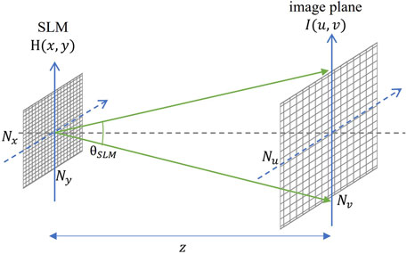
FIGURE 2. Lensless holographic projection geometry.

We focus on complex field information that produces graticule images at the image plane of different shapes and sizes for different measurement requirements like sample alignment, size or shape comparison, or area counting of a specimen. However, the sampling intervals here are constrained by Nyquist theory. To counter this limitation, we have two most common approaches. The first method increases the number of pixels while keeping the sampling pitch as defined in Eq. 4. However, the computation cost will increase in terms of time and memory. Nevertheless, we can use Eq. 1 for sampling limitation, but again it is not computationally efficient as it does not use FFT. Second, we can consider variable sampling intervals at the SLM and the reconstructed image plane by keeping the number of pixels, $N$ same in both planes. For this purpose, we use the scaled and shifted Fresnel diffraction algorithm, which computes the scaled Fourier transform by imposing a convolution theorem to the discrete 2D Fresnel diffraction algorithm as well as the off-axis image reproduction scheme by offsetting the target image plane from the optical axis to separate it from the DC term. The complex field is expressed as

$\mathit{I}\left(\mathit{u}\prime ,\mathit{v}\prime \right)={\mathit{C}}_{\mathit{z}}\mathit{ }.\mathit{\ast }{\mathit{F}}^{-1}\left\{\mathit{F}\left[\mathit{a}\left(\mathit{x}\prime ,\mathit{y}\prime \right)\right]\mathit{F}\left[\mathit{b}\left(\mathit{x}\prime ,\mathit{y}\prime \right)\right]\right\}(5)$

where the details for ${\mathit{C}}_{\mathit{z}}$, $\mathit{a},$ and $\mathit{b}$ are given in (Zhang et al., 2019). Here, $\mathit{x}\prime ={\mathit{x}}_0+\mathit{x}{\mathit{\Delta }}_{\mathit{SLM}}$, $\mathit{y}\prime ={\mathit{y}}_0+\mathit{y}{\mathit{\Delta }}_{\mathit{SLM}}$, $\mathit{u}\prime ={\mathit{u}}_0+\mathit{u}{\mathit{\Delta }}_{\mathit{I}}$, and $\mathit{v}\prime ={\mathit{v}}_0+\mathit{v}{\mathit{\Delta }}_{\mathit{I}}$ to represent the offset parameters ${\mathit{x}}_0$, ${\mathit{y}}_0$, ${\mathit{u}}_0$, and ${\mathit{v}}_0$ in offsetting the holographic image from the optical axis to separate the DC and conjugate terms from the target image. The algorithm is fast, keeping the same number of pixels, and involves three FFTs. Unfortunately, aliasing error may occur when propagating to a short distance. This is due to the diffraction angle, ${\theta }_{SLM}$ limited by the pixel pitch of the SLM expressed as

${\mathit{\theta }}_{\mathit{SLM}}={\mathit{s}\mathit{i}\mathit{n}}^{-\mathbf{1}}\left(\frac{\mathit{\lambda }}{{\mathit{\Delta }}_{\mathit{SLM}}}\right)\approx \frac{\mathit{\lambda }}{{\mathit{\Delta }}_{\mathit{SLM}}}(6)$

The projected image size is limited by

${\mathit{L}}_{\mathit{I}\_\mathit{max}}={\mathit{N}}_{\mathit{I}}{\mathit{\Delta }}_{\mathit{I}}\le \frac{\mathit{\lambda z}}{{\mathit{\Delta }}_{\mathit{SLM}}}(7)$

where the relation shows the image size is proportional to propagation distance and inversely proportional to the pixel pitch of SLM. To avoid an aliasing error by keeping the projected image size unchanged, the shorter propagation distance requires a much smaller sampling pitch, which is usually constrained by the pixel pitch of the physical SLM used in the experiment.

3D Layer-Based Hologram With Varying DOF

We need to reconstruct a holographic graticule to measure the sample on the microscope stage in a lateral and longitudinal direction. Lateral measurement is done in any planar dimension for the sample at the microscopic stage. It requires an enlarged DOF due to the sweeping of focal planes across the magnified sample image. On the other hand, longitudinal measurement requires a shallow DOF to axially evaluate the thickness and depth estimation of the magnified sample image.

The minimum angular spectrum range can be used to have enlarged or extended DOF. This can be done by multiplying the target image with a slowly varying spherical converging phase as in the random-phase-free method (Makowski et al., 2016a). In this way, the low-frequency information of a larger image can be spread to the hologram of a smaller size. The DOF is extended as each point in the image is formed by the limited circular effective aperture of the calculated hologram. The holographic image remains in focus in all focal planes, as illustrated in Figure 3.

FIGURE 3

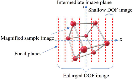
FIGURE 3. Illustration of enlarged and shallow DOF around intermediate image plane.

To have a shallow DOF, we can generate a hologram at a maximum angular spectrum range limited by the pixel pitch of the SLM. This can be done by multiplying a target image with the random phase distribution. We calculate the 3D hologram in a layer-based manner with 2D images reconstructed at different focal planes across the intermediate image plane with shallow DOF. The distance between layers is fixed to evaluate sample thickness while sweeping through different focal planes. Each layer has its sampling intervals defined based on the distance from the hologram plane in the scaled and shifted Fresnel diffraction algorithm. Finally, we follow the algorithm discussed in the previous section to obtain corresponding holograms for the extended and shallow DOF. The obtained two holograms are added together to form the final hologram which is then encoded to the phase hologram before being uploaded to the SLM. Other methods such as Gerchberg-Saxton (GS) algorithm (Chang et al., 2015) or error diffusion method (Jiao et al., 2020) can be applied to the accumulated complex field for the optimization of phase-only hologram.

Aliasing Condition

To avoid aliasing error in the lensless optical configuration under consideration, the convergent angle of the spherical phase in calculating an enlarged DOF should not exceed the diffraction angle limit of the SLM. The focal length, $\mathit{ f}$ of the spherical phase can be set for the propagation distance, $\mathit{z}$ considering the hologram size and image size as

$\mathit{f}=\frac{\mathit{z}}{1-\frac{{\mathit{L}}_{\mathit{h}}}{{\mathit{L}}_{\mathit{I}}}\mathit{ }}(8)$

where $\mathit{f}$ is proportional to the propagation distance, $z,$ and inversely proportional to the hologram size at the SLM plane.

In Figure 4, the blue line shows the maximum diffraction angle limited by the given SLM, and the red line shows the angle of a convergent spherical phase. Figure 4A shows the geometry model where the hologram fits perfectly inside the converging spherical phase with $\varphi ={\mathit{\theta }}_{\mathit{SLM}}$. Figure 4B shows the geometry model in which $\varphi <{\mathit{\theta }}_{\mathit{SLM}}$. Although some part of the SLM area is used, the image can be reconstructed without aliasing. Figure 4C shows the case for aliasing where $\varphi >{\mathit{\theta }}_{\mathit{SLM}}$, the information from the image reaching the SLM exceeds its total area. However, the image will still be reconstructed with aliasing noise due to the feature of the Fresnel diffraction algorithm. The bottom row of Figure 4 shows the numerically reconstructed result to demonstrate the aliasing effect.

FIGURE 4

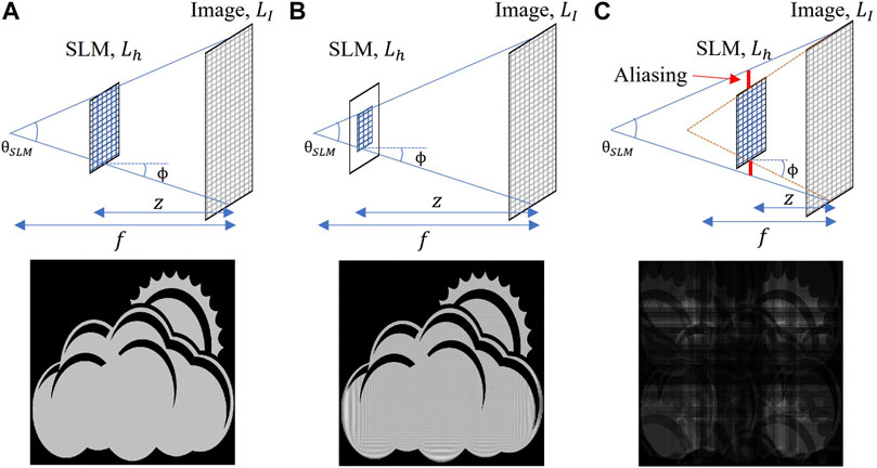
FIGURE 4. Aliasing condition for implemented holographic projection geometry. (A) Geometric projection model when $\varphi ={\theta }_{SLM}$ (no aliasing). (B) Geometric projection model when $\varphi <{\theta }_{SLM}$ (no aliasing). (C) Geometric projection model when $\varphi >{\theta }_{SLM}$ (aliasing occurs).

Numerical Simulation

In the numerical simulation, a holographic content is generated and centered around an intermediate image plane at the desired propagation distance, $\mathit{z}$. Two holograms are calculated for the extended and shallow DOF, respectively. The hologram with the extended DOF remains in focus over a large depth range with a slowly varying spherical phase distribution. On the other hand, the hologram with the shallow DOF is calculated in a layer-based fashion with layers having a random phase distribution and are separated by a particular distance. These two holograms are then accumulated in a single hologram for the numerical simulation results in Figure 5.

FIGURE 5

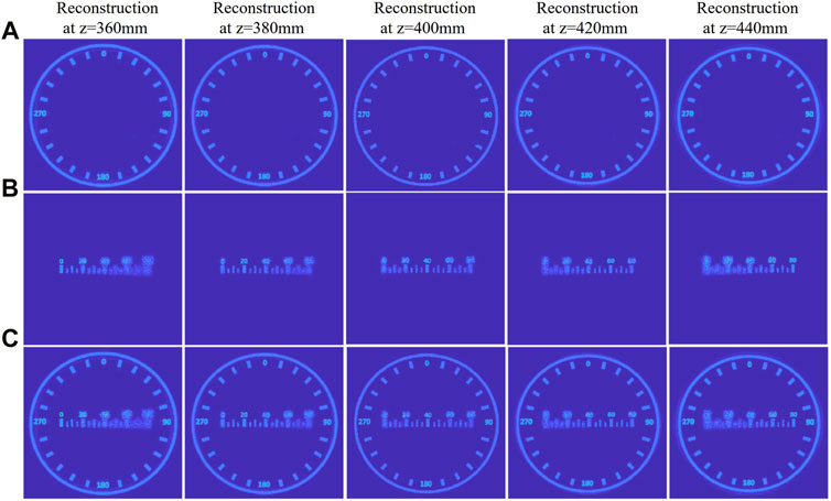
FIGURE 5. Numerical simulated results. (A) Reconstruction results at different planes show enlarged DOF. (B) Reconstruction results at different planes show shallow DOF. (C) The reconstruction results of the combined hologram at different planes simultaneously showed enlarged and shallow DOF.

The pixel resolution of the computation window used in the simulation is identical for the hologram and the target image plane, which is $\mathit{N}\times \mathit{N }= 2160\times 2160$ pixels. The sampling rate on the hologram plane is 3.6 um (which gives the size of the hologram, ${\mathit{L}}_{\mathit{h}}$ to be about 7.7 mm $\times$ 7.7 mm). The propagation distance, $\mathit{z}$ is 400 mm. The sampling rate of the reconstructed image at an intermediate image plane is about 32um. The wavelength of light is 633 nm.

Figure 5A shows the reconstructed results for a hologram synthesized with enlarged DOF at different focal planes. The image can be seen as a sample alignment graticule, each division with an angular separation of 15 degrees. We can see that the image is reconstructed with enlarged DOF. Figure 5B shows the results for a layer-based hologram synthesized for having a shallow DOF. Here, we have five 2D layers with numbers showing 0, 20, 40, 60, and 80 centered around an intermediate image plane spanning 80 mm longitudinal depth with the separation of 20 mm between each layer. Depending on the maximum angular range defined by the SLM, the separation between each layer can be increased or decreased, making the final reconstructed image show reasonable blur among different layers. The reconstructed scene here can be used for the depth estimation of a magnified sample image at the microscopic stage. As the reconstruction depth increases from left to right, different numbers in layers come into focus at a particular distance. Figure 5C shows the reconstructed results for an accumulated hologram at different reconstruction planes.

For the quantitative evaluation of the reconstructed holographic images at different planes for the enlarged DOF, we used two metrics: peak-signal-to-noise ratio (PSNR) and structural similarity index (SSIM). Table 1 shows the results. ${\mathit{T}}_1$, ${\mathit{T}}_2$, ${\mathit{T}}_3$, ${\mathit{T}}_4$ and ${\mathit{T}}_5$ represents the reconstructed image results in Figure 5A (top row) respectively. It can be seen from Table 1 that the highest quality is at the intermediate image plane ($\mathit{z}$ = 400 mm), and the quality degrades slowly while sweeping across the intermediate image plane.

TABLE 1

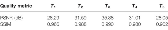
TABLE 1. Image quality measurement using PSNR and SSIM.

Experimental Results

Figure 6 shows the experimental optical setup for the lensless holographic and reflected bright-field microscopic configurations. In Figure 6A, the hologram is loaded to a spatial light modulator (SLM) after the phase encoding. We shifted the target image to separate it from the DC and conjugate term at the reconstruction plane. The reconstructions are captured around the intermediate image plane or CCD at a distance of 400 mm from the SLM plane. The wavelength of the laser light source used in the experiment is 633 nm. The reflection-type phase modulating SLM (model name: IRIS-U62) from MAY DISPLAY is used in the experiment that has the specifications of 3.6 um pixel pitch and 3840 $\times$ 2160 resolution. A hologram with enlarged DOF is synthesized with a slowly varying converging spherical phase, and a layer-based hologram with a shallow DOF is synthesized with a random phase distribution in each layer. Holograms are synthesized for the same pixel resolution of 2160 $\times$ 2160 as used in the numerical simulation. Finally, the two holograms are accumulated. In the encoding process, for the phase modulating SLM, the phase part of the final hologram was extracted and loaded to the SLM.

FIGURE 6

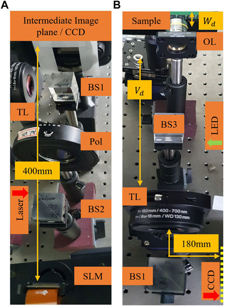
FIGURE 6. Optical experimental setup. (A) Lensless holographic configuration. (B) Reflected bright-field optical microscopic configuration.

In Figure 6B, we used an infinity-corrected plan achromatic objective lens (OL) of design magnification of ×10 at the working distance, ${\mathit{W}}_{\mathit{d}}$ of 1.2 mm from a sample stage. A tube lens (TL) of the effective focal length of 180 mm is used, designed for the infinity-corrected objective lens used in the experiment. The tube lens focuses the magnified sample image on the intermediate image plane. With such an arrangement of using an infinity-corrected objective lens and the tube lens, we obtain the variable distance, ${\mathit{V}}_{\mathit{d}}$ that is useful in positioning additional optical components. We used a M530L3 LED from Thorlabs as an incoherent light source with a wavelength centered around 530 nm. We used Kohler’s illumination technique to eliminate the source image at the CCD plane.

Figure 7 shows the optical experimental results. The phase part of the accumulated hologram, $\mathit{H}(\mathit{x},\mathit{ y}),$ used in the reconstruction process is shown in the top-left image. Figures 7A–E shows the reconstructed image results at various distances, i.e., 360–440 mm, with 20 mm separation from the SLM plane.

FIGURE 7

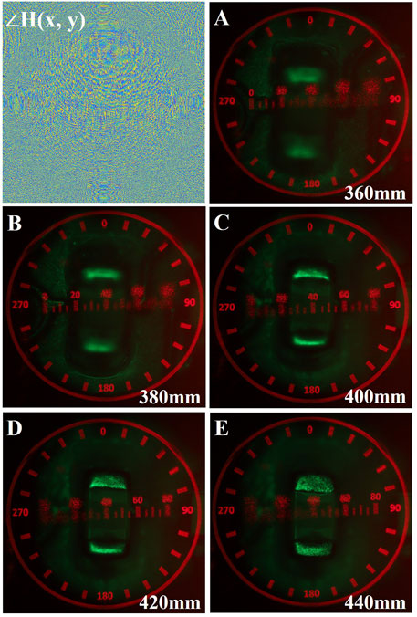
FIGURE 7. Optical experimental results. Top-left image shows the phase part of the accumulated hologram synthesized using the proposed method. (A–E) Different parts of the magnified sample image focus on the holographic image content at 360 mm, 380 mm, 400 mm, 420 mm, and 440 mm, respectively.

In Figure 7A, no part of the magnified sample image comes in focus with the holographic image number “0” (at 360 mm). At the distance of 380 mm in Figure 7B, the bottom part of the magnified sample focuses on the holographic image number “20”. By moving the CCD plane on the longitudinal axis further away from the SLM plane, different parts of the magnified sample image come into focus with the contents of holographic images. At the distance of 440 mm in Figure 7E, the top part of the sample focuses on the holographic image showing the number “80”. From this, we can analyze that the approximate thickness of the magnified sample is around 60 mm, from when the bottom part comes in focus at 380 mm up to the top part at 440 mm. As the longitudinal magnification of the magnified sample image is square of the lateral’s magnification, which is ×10 in our case, the magnified sample image has a longitudinal magnification of 100 times. From this, the total thickness of the sample approximates about 60 mm/100 (0.60 mm). The object sample we used is the multilayer ceramic capacitor from Samsung Electro-Mechanics (SEMCO) with the product code (CL05) having a thickness of 0.60 $\pm$ 0.10 mm, which is in good agreement with the experimental result. The error in the longitudinal measurement from the holographic graticule comes from the total number of 2D layers used in the hologram synthesis. As the layers are separated by 20 mm each, the maximum error in the longitudinal measurement of the object sample could be around $\pm$ 20 mm. By increasing the number of layers used in the layer-based hologram synthesis, we can minimize the error but at the cost of higher computation. The outer circular part of the holographic image shows the 360-degree alignment graticule with a 15-degree angular separation between each bar. We can see that it remains in focus at all reconstruction depths showing enlarged DOF.

Concluding Remarks

We proposed an augmentation of a 3D holographic content with the microscopic image to have an application of measurement graticule for a microscopic sample in lateral and longitudinal directions. This is done by combining two holograms synthesized for having an enlarged and shallow DOF. The optical geometry we used is the lensless holographic projection for its compactness and production of high contrast images. It is also easy to augment such a system with the conventional optical microscope as it requires no additional lenses between SLM and the projection screen to avoid lens aberrations. We have discussed aliasing conditions for considered projection geometry to avoid discrepancies with high-order diffracted results. Finally, we combined the two holograms and presented the numerical and experimental results to verify the proposed augmentation of the two systems.

Data Availability Statement

The raw data supporting the conclusions of this article will be made available by the authors, without undue reservation.

Author Contributions

MA conceived the idea, conducted the experiments, and wrote the manuscript. J-HP reviewed the experimental results and supervised this project. The manuscript has been revised and corrected by all authors.

Funding

This research was supported by the National Research Foundation of Korea (NRF) grant funded by the Korea Government (MSIT) (2022R1A2C2013455).

Conflict of Interest

The authors declare that the research was conducted in the absence of any commercial or financial relationships that could be construed as a potential conflict of interest.

Publisher’s Note

All claims expressed in this article are solely those of the authors and do not necessarily represent those of their affiliated organizations, or those of the publisher, the editors and the reviewers. Any product that may be evaluated in this article, or claim that may be made by its manufacturer, is not guaranteed or endorsed by the publisher.

References

Buckley, E. (2011). Holographic Laser Projection. J. Disp. Technol. 7 (3), 135–140. doi:10.1109/jdt.2010.2048302

CrossRef Full Text | Google Scholar

Chang, C., Xia, J., Yang, L., Lei, W., Yang, Z., and Chen, J. (2015). Speckle-Suppressed Phase-Only Holographic Three-Dimensional Display Based on Double-Constraint Gerchberg-Saxton Algorithm. Appl. Opt. 54 (23), 6994–7001. doi:10.1364/ao.54.006994

PubMed Abstract | CrossRef Full Text | Google Scholar

Goodman, J. W. (2005). Introduction to Fourier Optics. Englewood, Colorado: Roberts and Co. Publishers.

Google Scholar

Ji, Y.-M., Yeom, H., and Park, J.-H. (2016). Efficient Texture Mapping by Adaptive Mesh Division in Mesh-Based Computer Generated Hologram. Opt. Express 24 (24), 28154–28169. doi:10.1364/oe.24.028154

PubMed Abstract | CrossRef Full Text | Google Scholar

Jiao, S., Zhang, D., Zhang, C., Gao, Y., Lei, T., and Yuan, X. (2020). Complex-amplitude Holographic Projection with a Digital Micromirror Device (DMD) and Error Diffusion Algorithm. IEEE J. Sel. Top. Quantum Electron. 26 (5), 2800108. doi:10.1109/jstqe.2020.2996657

CrossRef Full Text | Google Scholar

Kim, H., Hahn, J., and Lee, B. (2008). Mathematical Modeling of Triangle-Mesh-Modeled Three-Dimensional Surface Objects for Digital Holography. Appl. Opt. 47 (19), D117–D127. doi:10.1364/ao.47.00d117

PubMed Abstract | CrossRef Full Text | Google Scholar

Lucente, M. E. (1993). Interactive Computation of Holograms Using a Look-Up Table. J. Electron. Imaging 2 (1), 28–34. doi:10.1117/12.133376

CrossRef Full Text | Google Scholar

Makowski, M., Ducin, I., Kakarenko, K., Suszek, J., and Kowalczyk, A. (2016a). Performance of the 4k Phase-Only Spatial Light Modulator in Image Projection by Computer-Generated Holography. Photonics Lett. Pol. 8 (1), 26–28. doi:10.4302/plp.2016.1.10

CrossRef Full Text | Google Scholar

Makowski, M., Shimobaba, T, and Tomoyoshi, I. (2016b). Increased Depth of Focus in Random-phase-free Holographic Projection. Chinese Optics Letters 14 (12), 120901–120905. doi:10.3788/col201614.120901

CrossRef Full Text | Google Scholar

McArthur, J. (1945). Advances in the Design of the Inverted Prismatic Microscope. J. R. Microsc. Soc. 65 (1‐4), 8–16. doi:10.1111/j.1365-2818.1945.tb00927.x

CrossRef Full Text | Google Scholar

McArthur, J. (1958). A New Concept in Microscope Design for Tropical Medicine. Am. J. Trop. Med. Hyg. 7 (4), 382–385. doi:10.4269/ajtmh.1958.7.382

PubMed Abstract | CrossRef Full Text | Google Scholar

Muffoletto, R. P., Tyler, J. M., and Tohline, J. E. (2007). Shifted Fresnel Diffraction for Computational Holography. Opt. Express 15 (9), 5631–5640. doi:10.1364/oe.15.005631

PubMed Abstract | CrossRef Full Text | Google Scholar

Shimobaba, T., Kakue, T., Masuda, N., and Ito, T. (2012). Numerical Investigation of Zoomable Holographic Projection without a Zoom Lens. Jnl Soc. Info Disp. 20 (9), 533–538. doi:10.1002/jsid.116

CrossRef Full Text | Google Scholar

Shimobaba, T., Makowski, M., Kakue, T., Oikawa, M., Okada, N., Endo, Y., et al. (2013). Lensless Zoomable Holographic Projection Using Scaled Fresnel Diffraction. Opt. Express 21 (21), 25285–25290. doi:10.1364/oe.21.025285

PubMed Abstract | CrossRef Full Text | Google Scholar

Wakunami, K., and Yamaguchi, M. (2011). Calculation for Computer Generated Hologram Using Ray-Sampling Plane. Opt. Express 19 (10), 9086–9101. doi:10.1364/oe.19.009086

PubMed Abstract | CrossRef Full Text | Google Scholar

Zhang, H., Cao, L., and Jin, G. (2019). Scaling of Three-Dimensional Computer-Generated Holograms with Layer-Based Shifted Fresnel Diffraction. Appl. Sci. 9 (10), 2118. doi:10.3390/app9102118

CrossRef Full Text | Google Scholar

Zhao, Y., Cao, L., Zhang, H., Kong, D., and Jin, G. (2015). Accurate Calculation of Computer-Generated Holograms Using Angular-Spectrum Layer-Oriented Method. Opt. Express 23 (20), 25440–25449. doi:10.1364/oe.23.025440

PubMed Abstract | CrossRef Full Text | Google Scholar