Multi-View Acoustic Field Imaging With Digital Color Holography

This paper proposes an approach for acoustic field imaging using simultaneous multi-view digital holography based on three-color digital off-axis holography. Considering spatio-chromatic multiplexing and the recording with a monochrome sensor, the numerical processing of time-sequences of holograms yields both the amplitude and phase of the acoustic field along three different directions of observation. Distortion analysis is presented and the acousto-optic interaction along the optical beam is discussed using a theoretical modelling. Experimental results with an emitter at 40 kHz establish the proof-of-concept of the proposed multi-view imaging for acoustic fields.

1 Introduction

The characterization and control of waves in acoustics, and more generally in wave physics, is of great interest because resulting technological innovations may impact several domains: environmental and energy transition (frugal engineering, lightening of structures, energy recovery, bio-sourced materials), health sector (medical imaging, remote consultation, diagnostic assistance), and industrial sector in the broadest sense (transportation, audio, musical instrument making, agriculture, electronics, and telecommunications). The characterization requires to develop new approaches to provide qualitative and quantitative insight of the acoustic fields of interest. Generally, imaging acoustic fields is performed by using microphone arrays (Flanagan et al., 1985; Hafizovic et al., 2012; Groschup and Grosse, 2015). Unfortunately, these methods intrinsically have several problems. Especially, microphone arrays have a low spatial resolution because the pitch of the microphones of the array is several millimeters (or more), and the presence of microphones may affect the acoustic field to be investigated.

In order to overcomes these limitations, optical techniques for measuring the acoustic field have been reported, for example, imaging with schlieren (Hargather et al., 2010), laser Doppler velocimetry (LDV) (Frank and Schell, 2005; Malkin et al., 2014), acousto-optic tomography (AOT) (Torras-Rosell et al., 2012), or laser feedback interferometry (LFI) (Bertling et al., 2014; Ortiz et al., 2018). Although schlieren simultaneously yields a collection of data points, its sensitivity to the air fluctuation due to acoustic wave is overall reduced because the approach is not directly sensitive to the refraction index of the medium. LDV, AOT and LFI are intrinsically sensitive to the refractive index of the medium in which the acoustic waves do propagate, but they require scanning to get a collection of data points. That makes these approaches less attractive than alternatives able to directly provide full-field data. Indeed, data acquisition and processing may be a critical issue for high-speed applications. Digital holography is a potential approach that can quantitatively measure the three-dimensional distribution of the refractive index of any transparent specimen or medium. This method takes a particular place because it records and retrieves the phase of the optical waves interacting with the medium (Schnars and Jüptner, 1994; Picart, 2015). Since the optical phase is closely related to the optical path difference, it includes the variation in the refractive index experienced by the light beam having crossed the acoustic field. Recent works reported the use of phase shifting digital holography (Yamaguchi and Zhang, 1997; Yamaguchi et al., 2002) to investigate acoustic waves (Matoba et al., 2014; Ishikawa et al., 2016; Ishikawa et al., 2018; Rajput et al., 2018; Ruiz et al., 2019; Takase et al., 2021; Hashimoto et al., 2022). Using off-axis digital holography (Picart, 2015), other authors reported the quantitative investigation of the acoustic field in acoustic wave guides (Penelet et al., 2016; Gong et al., 2018). However, acoustic wave guides are a particular case and the case of free space acoustic fields has to be investigated.

In this paper, we aim at demonstrating the proof-of-concept of simultaneous full-field and multi-view imaging of acoustic field in the free space using digital color holography and a single monochromatic high-speed sensor. The simultaneous acquisition of the necessary set of data is thus realized “single shot” and then numerical process yields images of both the amplitude and phase of the acoustic field along three different directions of observation. This has for advantage of permitting consistent and rapid data acquisition. The paper is organized as follows. Section 2 presents the theoretical basics of digital holography and spatio-chromatic multiplexing of holograms, Section 3 presents the amplitude and phase retrieval of the acoustic field along each view and discusses on the distortion in the measurement and Section 5 discusses on the experimental results obtained with the proposed method. Finally, Section 6 draws conclusions about the study.

2 Theoretical Basics

2.1 Off-Axis Hologram Recording and Reconstruction

In this paper, one considers off-axis digital holograms. This approach is the most adapted to dynamic events, especially to the investigation of acoustic fields which are time-varying. Recording a single hologram per time instant is powerful for carrying out high-speed data acquisition. At the sensor plane, the reference wave $\mathcal{R}$ is mixed with the wave $\mathcal{O}$ from the probed area to produce the digital hologram, expressed as,

$\mathcal{H}=|\mathcal{R}{|}^2+|\mathcal{O}{|}^2+{\mathcal{R}}^{\ast }\mathcal{O}+\mathcal{R}{\mathcal{O}}^{\ast }.(1)$

Note that term ${\mathcal{R}}^{\ast }\mathcal{O}$ refers to the +1 order of the hologram, and is considered in this paper. In the off-axis arrangement, the reference wave impacts the image sensor with an angle. Thus, the reference wave can be written as follows (a_λ is considered as constant and (u_λ, v_λ) denotes spatial frequencies, at wavelength λ):

$\mathcal{R}\left(x,y\right)=a_{\lambda }\exp \left(2i\pi \left(u_{\lambda }x+v_{\lambda }y\right)\right).(2)$

The recovery of the complex-valued amplitude of the image of the object is obtained by filtering the +1 order in the Fourier spectrum of the hologram. Filtering can be written as follows to yield the recovered complex image (FT means Fourier transform):

$A_r=a_r\exp \left(i{\phi }_r\right)={\mathcal{R}}^{\ast }\mathcal{O}\simeq {\text{FT}}^{-1}\left[\text{FT}\left[\mathcal{H}\right]\times G\right].(3)$

Equation 3 is a convolution formula, and the transfer function G is given by the bandwidth-limited angular-spectrum transfer function in the Fresnel approximation:

$G\left(u,v\right)=\left\{\begin{array}{cc}\hfill & \exp \left(-i\pi d_r\lambda \left({\left(u-u_{\lambda }\right)}^2+{\left(v-v_{\lambda }\right)}^2\right)\right)\hfill \\ \hfill & \text{if}|u-u_{\lambda }|\le \mathrm{\Delta }{u}_{\lambda }/2\text{and}|v-v_{\lambda }|\le \mathrm{\Delta }{v}_{\lambda }/2\hfill \\ \hfill & 0\text{if\hspace{0.17em}not.}\hfill \end{array}\right.(4)$

In Equation 4, (Δu_λ, Δv_λ) are the cut-off spatial frequencies for wavelength λ, and d_r is the refocus distance between the sensor and the area of interest. The spatial bandwidth of the filtering must be adapted to the extension of the +1 order to be filtered, and not too large in order to avoid over-sensitivity to noise. In (Gong et al., 2021), the noise standard deviation of the phase φ_r was demonstrated to be depending on the spatial bandwidths according to Eq. 5 (with the hypothesis of white noise),

${\sigma }_{\phi }=\frac{2\sqrt{p_x{p}_y\mathrm{\Delta }{u}_{\lambda }\mathrm{\Delta }{v}_{\lambda }}}{m\alpha N_{\mathit{sat}}}\sqrt{\alpha N_{\mathit{sat}}+{\sigma }_{ro}^2+\frac{N_{\mathit{sat}}^2}{12{\left(2^{nb}-1\right)}^2}},(5)$

where (p_x, p_y) are the pixel pitches of the sensor, m the modulation of the hologram, α the saturation rate of the hologram, N_sat is the maximum number of photo-electrons in the pixels, σ_ro is the read out noise and nb is the number of bits of the sensor. So, in order to minimize the noise in phase data, one has to increase m, α and to minimize (Δu_λ, Δv_λ). It follows that (Δu_λ, Δv_λ) have to be carefully chosen.

2.2 Multiplexed Three-Wavelength Digital Holography

Multi-view digital holography was discussed in literature and several architectures were proposed and demonstrated to be quite efficient for information encoding (Seo et al., 2007; Shaked et al., 2009; Shimobaba et al., 2010; Takaki, 2015; Ren et al., 2019). In this paper, we aim at considering multi-color digital holography. The use of three-wavelength digital holography has advantages compared to single-wavelength holography because it makes it possible to multiplex data from different sight views of the volume under interest. Having three laser beams at three different wavelengths generating three probe beams and three reference beams enable simultaneously recording the complex-valued data from three different sight-views in a single three-color hologram. The basic principle is depicted in Figure 1A with three laser beams propagating in the measurement volume along three different directions, and the probe beams being then combined with the three reference beams at the sensor plane. The reference waves have different incident angles in order to provide different spatial frequencies (u_λ, v_λ). Figure 1B illustrates the power spectrum density of the spatially-multiplexed three color hologram. Note that the simultaneous recording of three holograms at three different wavelengths has for consequence to increase the sensitivity to noise. Indeed, the total number of photo-electrons available for one single hologram is now divided by three, to be equal to N_sat/3. Considering Eq. 5, σ_φ is thus increased.

FIGURE 1

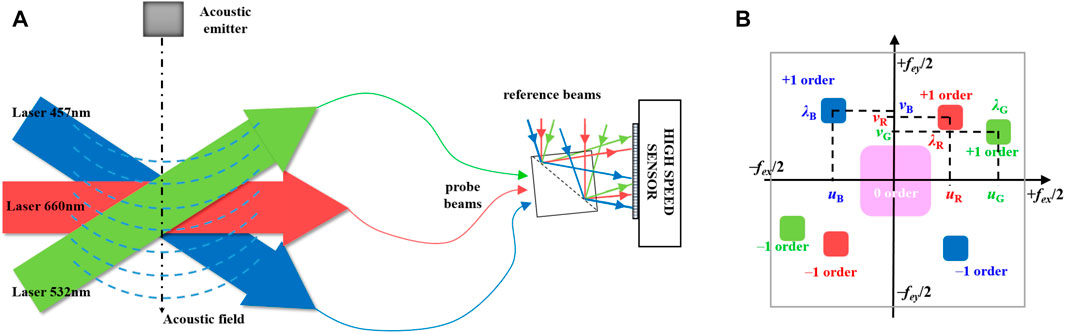
FIGURE 1. (A) Basic scheme for probing the acoustic field along three different directions with off-axis three color holography, (B) spectral distribution of the multiplexed off-axis digital holograms in the Fourier domain with three wavelengths (f_ex and f_ey refer to the spatial sampling frequencies of the sensor, i.e., f_ex = 1/p_x and f_ey = 1/p_y).

2.3 From Optical Phase to Acoustic Pressure

The laser beam crossing the acoustic field generated by any emitter (refer to Figure 1B) is perturbed by the acoustic pressure at any point in the propagation medium. The phase φ_r is related to the refractive index n_O (s, t) along the light path s according to the integral relationship Eq. 6.

${\phi }_r=\frac{2\pi }{\lambda }{\int }_L\left(n_O\left(s,t\right)-n_R\right)ds,(6)$

with n_R the reference refractive index along the reference optical path. So, the holographic measurement provides an average value of the refractive index along the interaction distance L. With help of the Gladstone-Dale relationship, the phase is related to the fluid density (Merzkirch, 2012). The density of the fluid at the pixels (x, y) of the image of the probed area is given by Equation 7 according to:

$\langle \rho \rangle \left(x,y,t\right)=\frac{2}{3\widehat{r}}\left(\langle n_O\rangle \left(x,y,t\right)-n_R\right).(7)$

In Equation 7, $\widehat{r}=0.1505\times 10^{-3}{\text{kg}}^{-1}.{\text{m}}^3$ is the specific refractivity of air measured at temperature 288 K and wavelength 660 nm (Merzkirch, 2012), which does not exhibits significant variation over the visible range of wavelengths. When air is submitted to the acoustic field, the air pressure fluctuates so that, holography measures, through the phase φ_r, the mean density ⟨ρ⟩ and the fluctuating component due to the propagation of the sound wave, ⟨ρ′⟩, included in the fluctuating part of phase, ${\phi }_r^{\prime }$. With the assumption of adiabatic process, the fluctuating part of the density is related to the pressure fluctuation, p′, according to (c₀ is the sound velocity in air) (Pierce and Beyer, 1990):

$p^{\prime }=⟨{\rho }^{\prime }⟩c_0^2=\frac{2}{3\widehat{r}}\frac{\lambda c_0^2}{2\pi L}{\phi }_r^{\prime }.(8)$

Note that in Equations 6, 8, L is the length of the line of sight. So, the value of L must be known in order to convert holographic phase data to acoustic pressure. In addition, in case where the acoustic field is not organized as plane waves, the effect of the interaction length with the laser beam is not straightforward to evaluate and requires minimum knowledge about the acoustic field.

3 Acoustic Amplitude and Phase Retrieval

3.1 Digital Synchronous Estimation

The optical phase extracted from the reconstructed object field, at any instant t, is given by,

$\psi \left(t\right)={\phi }_r+{\phi }_r^{\prime }\left(t\right)={\phi }_r+{\phi }_{ac}\sin \left({\omega }_{ac}t+{\varphi }_{ac}\right),(9)$

where φ_ac is the phase due to the acoustic fluctuation, and according to Eq. 8, is equal to:

${\phi }_{ac}=\frac{3\widehat{r}}{2}\frac{2\pi L}{\lambda }\frac{p_{ac}}{c_0^2},(10)$

with p_ac is the maximum acoustic pressure at pulsation ω_ac (period is T_ac = 1/f_ac, and f_ac the acoustic frequency) and ϕ_ac is the acoustic phase. Considering a time-sequence at sampling rate f_s = 1/T_s, including n_h digital holograms, the phase difference between two consecutive instants t_n+1 = (n + 1)T_s and t_n = nT_s is thus,

$\mathrm{\Delta }{\psi }_n=\psi \left(t_{n+1}\right)-\psi \left(t_n\right)=2{\phi }_{ac}\sin \left(\beta \pi \right)\cos \left({\varphi }_{ac}\right)\cos \left(\left(2n+1\right)\beta \pi \right)-2{\phi }_{ac}\sin \left(\beta \pi \right)\sin \left({\varphi }_{ac}\right)\sin \left(\left(2n+1\right)\beta \pi \right).(11)$

In Equation 11, β = T_s/T_ac. From Equation 11, both φ_ac and ϕ_ac can be retrieved by L2 norm minimization. Equation 11 can be approached with matrices. So, matrix X corresponds to known theoretical coefficients, vector Δψ includes the measured phase differences and vector y includes the two unknown (φ_ac, ϕ_ac) to be retrieved. We have $\mathit{y}={\left[\begin{array}{cc}\hfill y_1\hfill & \hfill y_2\hfill \end{array}\right]}^T$ (upper script T meaning transpose matrix), with $y_1=2{\phi }_{ac}\sin (\beta \pi )\cos \left({\varphi }_{ac}\right)$ and $y_2=2{\phi }_{\text{ac\hspace{0.17em}}}\sin (\beta \pi )\sin \left({\varphi }_{ac}\right)$. From Equation 11, matrix X is explicated according to:

$\mathit{X}=\left(\begin{array}{cc}\hfill \cos \left(\beta \pi \right)\hfill & \hfill -\sin \left(\beta \pi \right)\hfill \\ \hfill \cos \left(3\beta \pi \right)\hfill & \hfill -\sin \left(3\beta \pi \right)\hfill \\ \hfill \cos \left(5\beta \pi \right)\hfill & \hfill -\sin \left(5\beta \pi \right)\hfill \\ \hfill \cdots \hfill & \hfill \cdots \hfill \\ \hfill \cdots \hfill & \hfill \cdots \hfill \\ \hfill \cdots \hfill & \hfill \cdots \hfill \\ \hfill \cos \left(\left(2n_h+1\right)\beta \pi \right)\hfill & \hfill -\sin \left(\left(2n_h+1\right)\beta \pi \right)\hfill \end{array}\right).(12)$

The minimization of the L2 norm leads to the estimation of y using the cost function J = (Δψ −Xy)^TI (Δψ − Xy). Minimizing according to the calculation of ∂J/∂y yields the optimal solution ${\mathit{y}}_{\mathit{opt}}={({\mathit{X}}^T\mathit{I}\mathit{X})}^{-1}{\mathit{X}}^T\mathit{I}\mathbf{\Delta }\mathbf{\psi }$, with I being the identity matrix. Finally, one gets ${\varphi }_{ac}={\tan }^{-1}\left(y_2/y_1\right)$ and ${\phi }_{ac}=\sqrt{\left(y_1^2+y_2^2\right)}/2\sin (\beta \pi )$. So, from the optical phase extracted from the hologram sequence can be retrieved the amplitude-phase (φ_ac) due to the acoustic fluctuation and its oscillating phase (ϕ_ac). In the next sections, the method for acoustic amplitude and phase retrieval refers to SoundRetrieval.

3.2 Distortion in the Measurement

When recording the hologram sequence, the exposure time of the sensor has a major role in the accuracy of the retrieved amplitude and phase of the acoustic field. Indeed, the instantaneous hologram is time-integrated by the image sensor. Consider ΔT the exposure time, then the effectively recorded hologram is given by:

${\mathcal{H}}_{\mathit{eff}}=|\mathcal{R}{|}^2+{\int }_{t_1}^{t_1+\mathrm{\Delta }T}\left(|\mathcal{O}\left(t\right){|}^2+{\mathcal{R}}^{\ast }\mathcal{O}\left(t\right)+\mathcal{R}{\mathcal{O}}^{\ast }\left(t\right)\right)dt.(13)$

The temporal integration in Equation 13 can be derived considering the acoustic fluctuation in Equation 9, so that we have:

$\begin{array}{ll}\hfill & {\int }_{t_1}^{t_1+\mathrm{\Delta }T}\exp \left(i{\phi }_{ac}\sin \left({\omega }_{ac}t+{\varphi }_{ac}\right)\right)dt\hfill \\ \hfill & =\mathrm{\Delta }T\sum _k{J}_k\left({\phi }_{ac}\right)\text{sinc}\left(k{\omega }_{ac}\frac{\mathrm{\Delta }T}{2}\right)\exp \left(ik\left({\omega }_{ac}{t}_1+{\varphi }_{ac}+\frac{{\omega }_{ac}\mathrm{\Delta }T}{2}\right)\right).\hfill \end{array}(14)$

Since the sinc function can be expanded as:

$\text{sinc}\left(k\pi \frac{\mathrm{\Delta }T}{T_{ac}}\right)=1+P\left(k\pi \frac{\mathrm{\Delta }T}{T_{ac}}\right)\text{with}P\left(x\right)=\sum _{n=1}^{n=\infty }{\left(-1\right)}^n\frac{x^{2n}}{\left(2n+1\right)!},(15)$

it follows that the time-averaging of the acoustic amplitude can be rewritten,

$\begin{array}{ll}\hfill & {\int }_{t_1}^{t_1+\mathrm{\Delta }T}\exp \left(i{\phi }_{ac}\sin \left({\omega }_{ac}t+{\varphi }_{ac}\right)\right)dt\hfill \\ \hfill & =\mathrm{\Delta }T\exp \left(i{\phi }_{ac}\sin \left({\omega }_{ac}{t}_1+{\varphi }_{ac}+\frac{{\omega }_{ac}\mathrm{\Delta }T}{2}\right)\right)+\mathrm{\Delta }Tq\exp \left(i\gamma \right),\hfill \end{array}(16)$

where q and γ both depend on the expansion of the sinc function according to:

$\gamma =\arg \sum _k{J}_k\left({\phi }_{ac}\right)P\left(k\pi \frac{\mathrm{\Delta }T}{T_{ac}}\right)\exp \left(ik\left({\omega }_{ac}{t}_1+{\varphi }_{ac}+\frac{{\omega }_{ac}\mathrm{\Delta }T}{2}\right)\right),(17)$

and

$q=\left|\sum _k{J}_k\left({\phi }_{ac}\right)P\left(k\pi \frac{\mathrm{\Delta }T}{T_{ac}}\right)\exp \left(ik\left({\omega }_{ac}{t}_1+{\varphi }_{ac}+\frac{{\omega }_{ac}\mathrm{\Delta }T}{2}\right)\right)\right|.(18)$

From Equations 3, 17, 18, the phase extracted from the hologram and due to the time average of the acoustic pressure from the temporal integration of the sensor is given by:

$\psi =\arg \left(A_r\right)={\phi }_r+{\psi }_{ac}-{\text{tan}}^{-1}\left(\frac{q\sin \left({\psi }_{ac}-\gamma \right)}{1+q\cos \left({\psi }_{ac}-\gamma \right)}\right),(19)$

with

${\psi }_{ac}={\phi }_{ac}\sin \left({\omega }_{ac}t+{\varphi }_{ac}+\frac{{\omega }_{ac}\mathrm{\Delta }T}{2}\right).(20)$

Equation 20 shows that the phase from the hologram includes the expected phase fluctuation from acoustics and a phase error which depends on both the acoustic phase fluctuation and the ratio between ΔT and T_ac. The phase error is given by:

${\psi }_{\mathit{err}}={\text{tan}}^{-1}\left(\frac{q\sin \left({\psi }_{ac}-\gamma \right)}{1+q\cos \left({\psi }_{ac}-\gamma \right)}\right).(21)$

The phase error can be high and may strongly distort the measured phase fluctuation. In order to illustrate the error generated by the temporal integration due to the exposure time, one considers those physical parameters: f_ac = 40 kHz, p_ac = 20 Pa, ϕ_ac = π/4, ΔT = 10 µs, λ = 660 nm, L = 50 mm, and c₀ = 340 m/s. Then, the optical phase fluctuation amplitude due to acoustics is φ_ac = 0.0185 rad ≃ 2π/340. The error is calculated using Eq. 21 and the distortion ratio of the amplitude φ_ac is estimated at τ_err = 100 × ψ_err/φ_ac = 24.3%.

Figure 2A shows the temporal acoustic oscillation with comparison with the exposure time and the acoustic period for the chosen parameters. In Figure 2B is displayed the comparisons between the acoustic oscillations in the ideal case (red curve, no distortion), the ideal case with phase shift ω_acΔT/2 (black curve, no distortion), and the acoustic oscillation distorted by the time-average of the exposure time (blue curve). The comparison between the simulated phase error by considering numerical integration of the ideal signal in Figure 2A and the theoretical expression (Eq. 21) is provided in Figure 2C. It can be observed that the theoretical expression very well fits the numerical estimation, thus validating the proposed theoretical approach. When considering the variation of the acoustic pressure from 5 to 150 Pa and exposure time varying from 1 to 10 µs, the distortion rate plotted versus the time-average ratio α = ΔT/T_ac is given in Figure 2D. It can be seen that the distortion rate mainly depends on the acoustic amplitude and that it may be larger than 30% for ratio ΔT/T_ac ≃ 0.6 and P_ac = 150 Pa. Note also that the measured acoustic oscillation includes a phase shift ω_acΔT/2 = απ compared to the emitted signal. This phase shift is irrelevant if α tends to 0, that is ΔT ≪ T_ac.

FIGURE 2

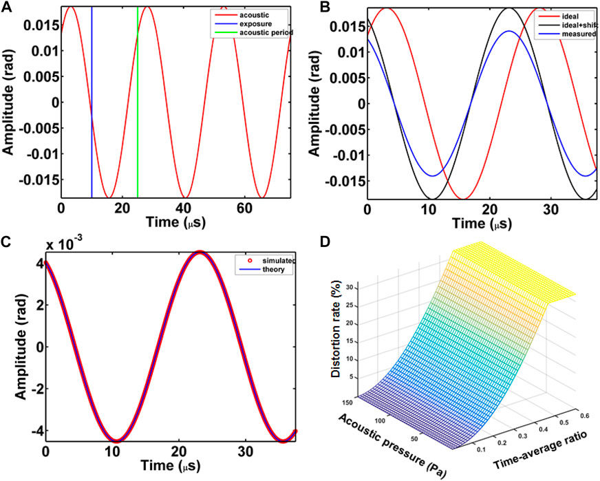
FIGURE 2. (A) Temporal acoustic oscillation with comparison with the exposure time and the acoustic period for f_ac = 40 kHz, ϕ_ac = π/4, and ΔT = 10 µs, (B) comparisons of acoustic oscillations, red: ideal as in (A), black: ideal with phase shift of ω_acΔT/2, blue: distorted by the time-average of the exposure time, (C) comparison between the simulated phase error and the theoretical expression from Eq. 20, (D) evolution of the distortion rate (%) versus the acoustic pressure from 5 to 150 Pa and the time-average ratio ΔT/T_ac for exposure time varying from 1 to 10 µs.

4 Experimental Set-Up

4.1 Three Color Digital Holographic Set-Up

The optical set-up is described in (Figure 3) Three continuous lasers at λ_R = 660 nm (300 mW), λ_B = 457 nm (150 mW) and λ_G = 532 nm (300 mW) are split into three reference beams and three illumination beams. Half wave plates for the three laser beams are used, namely, λ_R/2 the half wave plate for the red laser, λ_G/2 the half wave plate for the green laser, and λ_B/2 that for the blue laser. These are used to adjust, on one hand, the amount of power in the reference and probe beams, and on the other hand, to turn the polarisation in the R-G-B reference beam so that interference may occur. The three reference beams are then combined into a single R-G-B beam using dichroic plates. The object volume is illuminated simultaneously along the different propagation directions by the red beam along the direct direction, “direct view”, along the orthogonal direction by the green beam, “orthogonal view”, and in one direction inclined from almost 21° for the blue beam, “tilted view”. Thus, three simultaneous illumination angles (0°, 21.31°, 90°) are produced. The measurement volume corresponds to the zone of space in which the three color laser probes are mixed. The volume is almost a sphere 20 mm in diameter localized at d_r ≃ − 1,310 mm from the sensor area. Each measurement and reference beam is spatially filtered and expanded to produce plane and smooth waves. Using beam splitter cubes, the six beams are recombined onto a high-speed camera (Photron SA-X2; nb = 12 bits) with a spatial resolution of 1,024 × 1,024 pixels at 12,500 fps. The pixel pitches of the sensor are p_x = p_y = 20 μm and the exposure time is set at ΔT = 1 µs, in order to avoid distortion from the time-averaging. The off-axis recording is adjusted by tilting cubes in order to produce the three different carrier frequencies along each viewing direction. This has for consequence that the monochrome recorded hologram includes three spatially multiplexed color holograms at each wavelength. It follows that the three color holograms can be separated in the Fourier spectrum of the digital hologram. The localized filtering with adapted spatial bandwidth (Δu, Δv) for each wavelength, permits to extract the complex images A_r along each view. Then, the temporal phase differences are calculated for each color and processed with the SoundRetrieval algorithm to get the amplitude and phase of the acoustic oscillation for each sight view. It follows that the set-up permits to simultaneously measure the amplitude and phase of the acoustic field along three different lines of views.

FIGURE 3

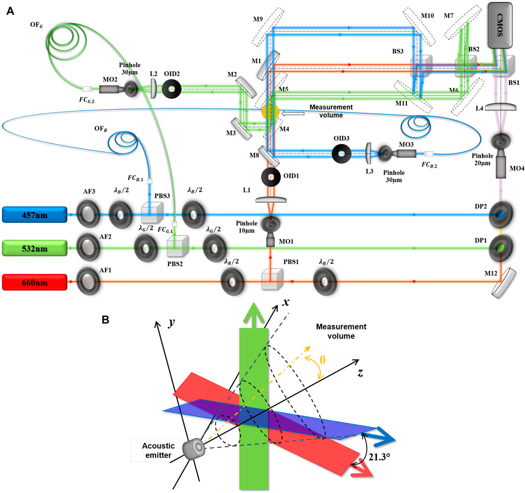
FIGURE 3. (A) Experimental set-up (AF: Attenuators, PBS: polarizing beam splitters, M: mirrors, DP: dichroic plates, MO: microscope objectives, FC: Fiber-optic collimators, OF: Optical fibers, BS: 50% beam splitter cube, OID: iris diaphragm, λ_R/2: half wave plate for the red laser, λ_G/2: half wave plate for the green laser, λ_B/2: half wave plate for the blue laser), (B) scheme of the measurement volume, the transducer emits acoustic waves and the three laser beams crosses the acoustic field at a certain distance from the emitter.

4.2 Acoustic Emitter Characterization

The acoustic field is generated using an acoustic emitter as an ultrasonic piezoelectric transducer (MA40S4S; diameter 9.9 mm). The transducer is localized at a few centimeter from the measurement volume and emits acoustic waves at frequency f_ac = 40 kHz and is driven by sinusoidal voltage (typ. 10V peak-to-valley). The acoustic wavelength is then λ_ac = c₀/f_ac = 8.5 mm. From the provider, the sound pressure may reach 120 dB in the far field (so almost 120 Pa). The characterization of the acoustic emitter is carried out using a microphone (GRAS 40BP 1/4” Ext. Polarized Pressure Microphone) which has a sensitivity of 1.6 mV/Pa over a frequency range 4–70 kHz and a dynamic range of 34–169 dB. The microphone is powered by a NEXUS conditioning amplifier type 2692-C linked to an oscilloscope to measure the amplitude of the sound pressure oscillations. In order to measure the sound pressure, or the sensitivity S delivered by the ultrasonic transducer, as a function of the angle θ of emission, the transducer is mounted on one rotating header. The microphone is also mounted on a static support in front of the center of the acoustic emitter. The transducer header is adjusted so that angle θ = 0 coincides with the maximum emission (acoustic signal is maximum). The sensitivity of the receiver is set at 1.651 mV/Pa. This value is considered as a reference acoustic pressure S_o. Table 1 gives the sensitivities calculated at different distances between the transmitter and the receiver in the sagital and parallel planes. The sensitivity is estimated by calculating $S(dB)=20\log \frac{S_v}{S_o}$, with S_v the measured microphone voltage at each emission angle. The sensitivities in Table 1 reach almost the 1,050 dB, which is measured at a reference sound pressure equal to 10 V/Pa. Note that for measuring such high sound pressure close to the emitter, the excitation signal was lowered so as to avoid saturation from the microphone and then the pressure was estimated by assuming linear behavior of the microphone. The experimental radiation patterns of the acoustic wave from the transducer are shown in Figures 4A,B, both at 40 kHz. The measurements of the voltages are carried out in the sagital and parallel planes. As expected, the piezoelectric emitter produces an almost Lambertian radiation, with a strong directivity in the central axis for both distances d = 90 mm and d = 100 mm. By comparing the measurements presented in the technical sheet carried out in an anechoic chamber and those presented in Figures 4A,B, we observe a relative error of 13.3% for the sensitivity measured at a distance d = 90 mm at both sagital and parallel planes. That is almost acceptable considering that our measurements were not realized in a perfectly controlled acoustic environment.

TABLE 1

TABLE 1. Sensitivities of the acoustic emitter MA40S4S at different distances.

FIGURE 4

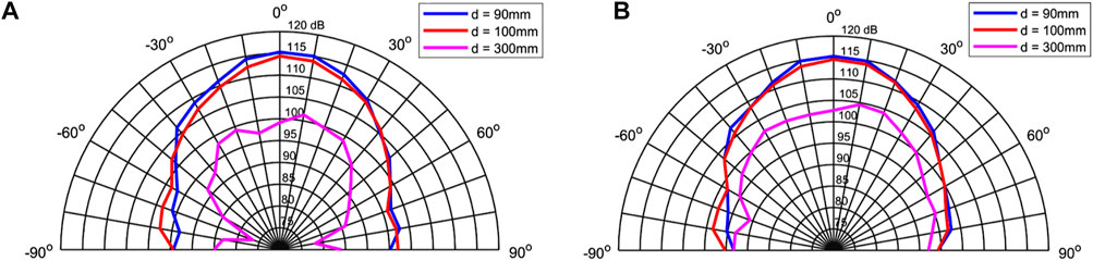
FIGURE 4. Directivity of the acoustic radiation of the ultrasonic transmitter (MA40S4S), (A) sagittal plane, (B) vertical plane.

5 Experimental Results

5.1 Spatio-Chromatic Multiplexed Hologram and Related Power Spectrum Densities

Figure 5A shows the recorded three-color digital hologram with exposure time set at 1 µs. In Figure 5B, a zoom of the digital hologram exhibits the fine structure of the hologram where the micro fringes related to each of the individual R, G and B colors are mixed to produce a kind of mosaic. The color bar in Figure 5A relates to gray levels of the digital hologram. The sensor has nb = 12 bits quantization, so the maximum value of the gray levels is 4095. In Figure 5A, the maximum value of the color bar is around 1000. It follows that digital holograms occupy almost 1/4 of the full sensor dynamics. In Figure 5C, the spatial frequency power spectrum density is displayed. The different orders along each color can be observed and they are marker with squares and related R-G-B letter. As can be seen, the +1 orders can be easily filtered since they are well separated in the power spectrum. The spatial frequencies of the centers of each order are (u_R, v_R) = (−17.76, −12.55) mm⁻¹ for the red laser, (u_G, v_G) = (+20.74, −18.66) mm⁻¹ for the green one and (u_B, v_B) = (+5.32, −15.52) mm⁻¹ for the blue laser. The filtering bandwidth according to Eq. 4 depends on the laser beam it follows that for the set-up, they were chosen to be Δu_R = Δv_R = 1.11 mm⁻¹, Δu_G = Δv_G = 2.17 mm⁻¹ and Δu_B = Δv_B = 0.83 mm⁻¹ respectively for the R-G-B beams. From the average amplitude of the +1 and 0 orders extracted from the numerical processing, along each color, the average modulation and saturation rate of the holograms can be estimated. For the red beam, (m, α) = (66, 7.6)%, for the green beam, (m, α) = (4.1, 6.1)% and for the blue one, (m, α) = (21, 3)%. As can be seen, the G hologram has the weakest modulation and this increases its sensitivity to noise, whereas the two others have reasonable modulation although the optimal modulation would be close to 1. The reason for average modulations is not clear in the set-up, although the beam polarisation and optical path difference are well managed. The B beam is saturated at only 3% and this is due to lack of laser power. Overall, the saturation rate of the three beams does not exceed 10%. Ideally, that would be better to be close to α ≃ 1/6, that is almost 16%. But considering the exposure time at 1 μs and the available average power per channel ($<$ 300 mW), such ratio is not reachable. Using the values of (m, α) and Eq. 5, the estimation of the standard deviation of noise can be given and correlated with the experimental estimation. This point is discussed in the next section.

FIGURE 5

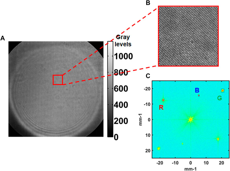
FIGURE 5. (A) Recorded three color hologram, (B) zoom of the hologram exhibiting the fine structure due to the spatio-chromatic multiplexing of the three R, G and B holograms, (C) power spectrum density of the three color hologram with the diffraction orders and the spatial bandwidth of the filtering; the useful +1 orders are framed by squares which correspond to the spatial filtering bandwidth.

5.2 Phase Noise Characterisation

The phase noise is characterized by recording a time sequence of digital color holograms without any acoustic wave in the measurement volume. Separately, in order to check the noise amount for each wavelength, a sequence of monochromatic holograms with duration 160 ms was recorded at frame rate 12,500 Hz (exposure time at 1 µs) to yield almost 2000 digital holograms. Then, for each R-G-B sequence, the phase differences ψ(t) are calculated and the standard deviations of noise are estimated. A region of 15 × 15 pixels at the center of the fields of view was selected to yield 225 temporal signals. The probability density function of the 225 signals is estimated. The power spectrum density [S_λ(ν)] of each signal was calculated using fast Fourier transforms (Oppenheim, 1999), and then averaged to yield $({\widehat{S}}_{\lambda }(\nu ))$. The standard deviation of noise over a spectral bandwidth was calculated according to:

${\sigma }_n={\int }_{f_1}^{f_2}{\widehat{S}}_{\lambda }\left(\nu \right)d\nu .(22)$

Figure 6 summarizes the results obtained for the three beams. In Figures 6A–C, the plots of the 225 temporal signals respectively along the R, G and B wavelength are displayed. The plots clearly shows that the phase fluctuation is the smallest in the R beam, whereas it is larger for the G, and more than π rad for the B beam. The R and B signals show that the noise fluctuations include deterministic parts whereas the G beam seems to be more randomly distributed. This is confirmed when considering Figures 6D–F which exhibit the probability density functions estimated from 225 signals for the R-G-B beams respectively. The G probability density function exhibits Gaussian shape, and none of the two others. The strong parasitic oscillation observed in the B channel is unexplained. In Figures 6G–I are plotted the average power spectrum densities of the set of signals for R-G-B respectively. As intuited by the temporal signals, the G spectrum is more related to white noise than the two others. According to these observations, the amount of pure noise can be estimated from both Eq. 5 and the averaged power spectrum densities. For the estimated values of (m, α) and (Δu_λ, Δv_λ) for the R-G-B holograms, with N_sat = 16,000 electrons, σ_ro = 27 electrons, nb = 12 bits, the theoretical standard deviation of noise was calculated to σ_φ,R = 0.0027 rad, σ_φ,G = 0.088 rad and σ_φ,B = 0.011 rad. The experimental standard deviation of noise was estimated with Eq. 22 for the bandwidth almost corresponding to white noise, between f₁ = 4,500 Hz and f₂ = 6,000 Hz, leading to σ_{φ,R− exp} = 0.0024 rad, σ_{φ,G− exp} = 0.094 rad and σ_{φ,B− exp} = 0.24 rad. So, it follows that for the R and G beams, the theoretical estimations are almost close to the experimental values in the white noise hypothesis. However, for the B beam, the difference is high because the hypothesis is broken since the bandwidth in the range (4,500, 6,000) Hz is not as flat as expected.

FIGURE 6

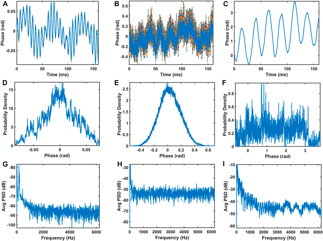
FIGURE 6. (A–C) Plots of a set of 225 temporal signals respectively along the red, green and blue beams, (D–F) probability density functions estimated from the set of signals for R-G-B respectively, (G–I) average power spectrum densities of the set of signals for R-G-B respectively.

5.3 Multi-Views of the Acoustic Field

The acoustic transducer was excited at 40 kHz and placed at different distances from the measurement volume, that are d = 0 mm, d = 90 mm, d = 100 mm and d = 200 mm. For distance d = 0 mm, that is the transducer is close to the measurement volume, the acoustic pressure was measured with the microphone at almost 1,050 Pa. Temporal sequences of digital color holograms were recorded with frame rate at 12.5 kHz and exposure time at 1 µs. At this frame rate, matrices of 1024 × 1024 pixels are recorded and α = 0.04. With f_ac = 40 kHz, the Shannon conditions for temporal sampling are not fulfilled, since the basic requirement would lead to sampling rate larger than 80 kHz. However, at 80 kHz, the spatial resolution would be drastically reduced. In order to keep a good spatial resolution at 1024 × 1024 pixels, the frame rate was voluntarily chosen less than the acoustic frequency. This requires to make adjustments of the parameters of the SoundRetrieval algorithm. Especially, since aliasing occurs, the acoustic frequency is observed at $f_{ac}^{\prime }=2500\text{Hz}$ in the power spectrum density. Considering Figure 6, the noise bandwidth becomes to be almost flat in this frequency band thus enabling the measurement of the acoustic frequency. Practically, one has to consider a virtual sampling period that depends on the ratio between the acoustic frequency and the actual sampling frequency, according to $T_s^{\prime }=T_s-k_s\times T_{ac}$, with k_s = floor (f_ac/f_s) (floor (…) meaning lower rounding). So, this yields the new virtual sampling frequency $f_s^{\prime }=1/T_s^{\prime }$ that is required for the SoundRetrieval. With the experimental parameters, we have k_s = 3, $T_s^{\prime }=5\times 10^{-6}\text{s}$, $f_s^{\prime }=200\text{kHz}$ to be injected in the sound retrieval method.

It follows from the previous section that the distortion rate is estimated 0.26% for α = 0.04 and phase amplitude ranging from 0.01 to 0.04 rad. So, it appears that for this range of α value and measured phase amplitude, there is no specific requirement for compensating for the distortion due to the time-average of the exposure time.

Figures 7A,C,E, 8A,C,E, 9A,C,E, 10A,C,E show the measured acoustic amplitude for respectively the red, green and blue channels for the excitation at f_ac = 40 kHz. The acoustic amplitude is expressed in radians rather than in pressure units. This point will be discussed in the next section. Figure 7B,D,F, 8B,D,F, 9B,D,F, 10B,D,F show the measured acoustic phase for respectively the red, green and blue channels. In Figures 7, 8, 9, 10, one clearly observes dark and bright fringes that demonstrate the existence of the acoustic wave in the free field. The acoustic wave is spherical when the transducer is close to the measurement volume (Figure 7). Then, it becomes to be plane wave far from the emitter as in Figure 8, 9, 10. Note that, the image quality along the G and B channels are lower than for the R channel and this in close correlation with Figure 6.

FIGURE 7

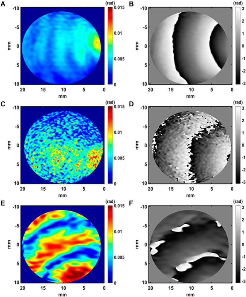
FIGURE 7. Amplitude and phase of the acoustic field at 0 mm, (A,B) along the R view, (C,D) along the G view, (E,F) along the B view.

FIGURE 8

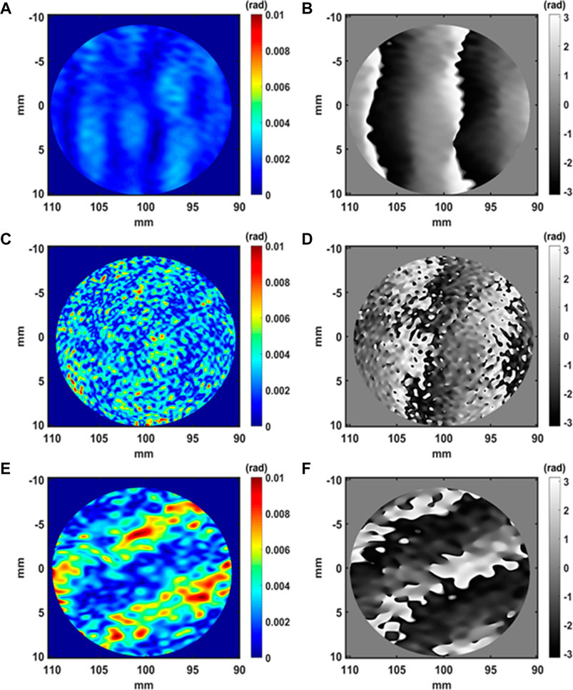
FIGURE 8. Amplitude and phase of the acoustic field at 90 mm, (A,B) along the R view, (C,D) along the G view, (E,F) along the B view.

FIGURE 9

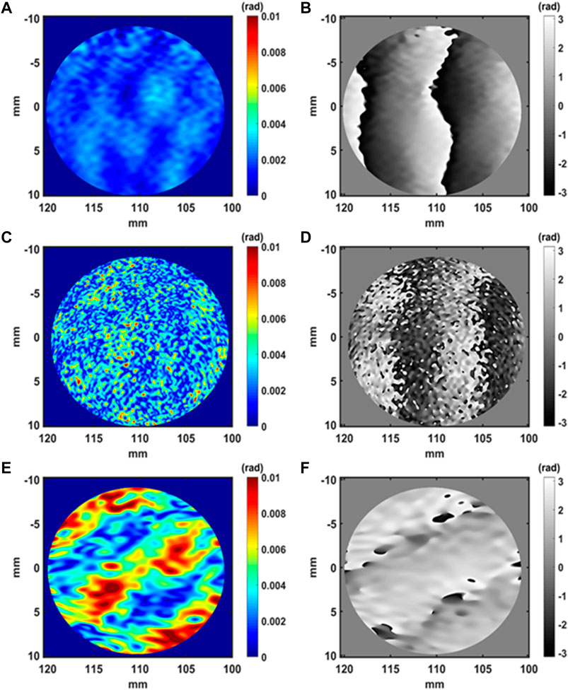
FIGURE 9. Amplitude and phase of the acoustic field at 100 mm, (A,B) along the R view, (C,D) along the G view, (E,F) along the B view.

FIGURE 10

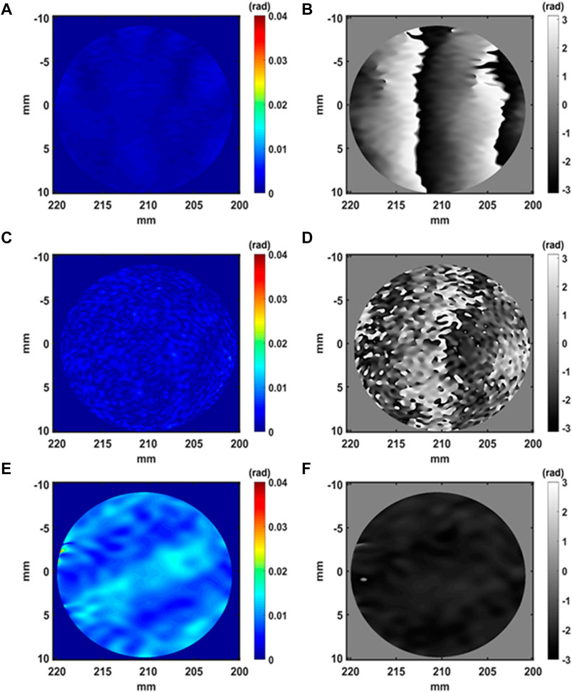
FIGURE 10. Amplitude and phase of the acoustic field at 200 mm, (A,B) along the R view, (C,D) along the G view, (E,F) along the B view.

If one considers Equation 10, then we can estimate the interaction length of the laser beam in the acoustic field as,

$L=\frac{2\lambda }{3\widehat{r}}\frac{c_0^2}{p_{ac}}\frac{{\phi }_{ac}}{2\pi }.(23)$

With the R channel at distance d = 0 mm, we can consider the measured value at φ_ac ≃ 0.010 rad (Figure 7A). With the physical parameters, the estimated value of the interaction length is L ≃ 0.5 mm. From Figure 7A we can estimate that the acoustic field seems to be extended on a width quite larger that L, at almost ≃ 4–5 mm. Thus, this result obtained by the holographic method seems to be not in agreement with the microphone measurement in the sound field. With Figure 9A, one can estimate that φ_ac ≃ 0.0040 rad. With the microphone at the center of the field at distance d = 100 mm, P_ac = 126 Pa, and one can then estimate L ≃ 1.07 mm. We see that the estimated interaction distance increases, which is expected since the transducer produces a divergent wave. However, considering the strong divergence of the acoustic beam, this value is probably not correct, as for distance d = 0 mm.

The maximum values of the acoustic amplitudes measured for the R, G and B at the different distances from the measurement volume (0, 90 mm, 100 mm, 200 mm) are presented in Table 2. This table requires a few comments. The amplitudes measured along the R-G-B channels follow a similar trend, except for channel B at distance 200 mm. Indeed, the measured amplitudes decrease with distance, which is expected for a spherical wave. For channel B at 200 mm, it is likely that the measurement is strongly influenced by noise because it should be lower than measurements at other distances, which is not the case. The measurements along G follow a consistent pattern although the maps of Figures 7 –10 appear to be the noisiest of all the measurements.

TABLE 2

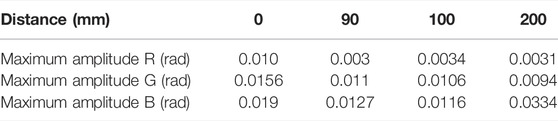
TABLE 2. The maximum values of the acoustic amplitudes measured for the R,G and B views at different distances from the measurement volume.

In order to investigate the noise contribution at f_ac = 40 kHz, the SoundRetrieval algorithm was applied to the noise sequence from the previous section. Figure 11 shows the amplitude and phase of the noise contribution at 40 kHz for the three R-G-B channels. The standard deviations along each noise amplitude map were estimated to σ_R = 8.23 × 10^–6 rad, σ_G = 4.63 × 10^–4 rad, and σ_B = 4.7 × 10^–5 rad. As mentioned before the red channel provides the lowest noise contribution to the acoustic measurement.

FIGURE 11

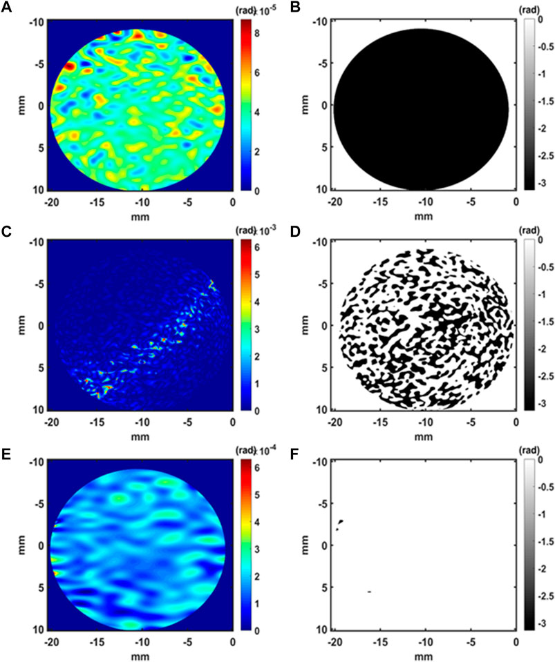
FIGURE 11. Amplitude and phase of the at f_ac = 40 kHz, (A,B) along the R view, (C,D) along the G view, (E,F) along the B view.

In Figures 7–10, phase jumps are observed in the phase map of the acoustic field. These indicate that each phase jump corresponds to change in the sign of the acoustic oscillation, in close relation with the acoustic wavelength as depicted in Figure 12A. Figure 12B plots the profile of the acoustic phase along the horizontal direction in the R measurement. From that, the acoustic wavelength is estimated to λ_ac−exp ≃ 8.86 mm and is close to the theoretical λ_ac = 8.5 mm. So the two wavelengths are in good agreement, confirming that the acoustic field is well measured by the holographic imaging system.

FIGURE 12

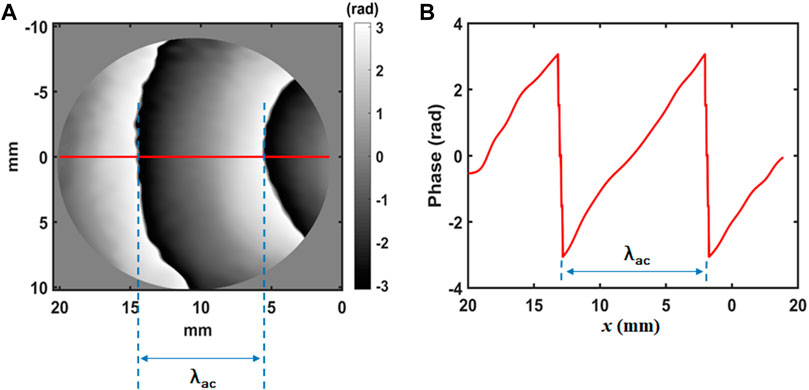
FIGURE 12. Acoustic wavelength measured along the R view, (A) scheme of the phase of the acoustic field at distance 0 mm, (B) Phase profile of the acoustic field along the x direction for an excitation frequency of 40 kHz.

6 Discussion

In this section, the acoustic field is recovered according to the theoretical basics described previously, that is integrated along the line of view of the laser beam. In order to qualitatively appraise the effect of the integration along the optical path and to evaluate the relevance of the results obtained in the previous section, simulations were carried out. The aim is to investigate the amplitude and the phase of the acoustic field when considering realistic simulations as close as possible to the experiments of the paper. The case of interest is that of non-plane acoustic wave. In the case of plane waves in an acoustic wave guide, the correspondence between the actual phase and the measured one is straightforward (Penelet et al., 2016; Gong et al., 2018; Gong et al., 2021). The simulation of the acoustic field was carried out for transducer as a rigid piston in a baffle with radius a = 4.95 mm, and executing harmonic oscillations at frequency f_ac = 40 kHz. The theoretical relation describing the acoustic field is given in Eq. 24 (Pierce and Beyer, 1990),

$p_{ac}\propto \frac{\exp \left(i{k}_{ac}r\right)}{r}\frac{J_1\left(k_{ac}a\sin \left(\theta \right)\right)}{k_{ac}a\sin \left(\theta \right)},(24)$

with k_ac = 2π/λ_ac the acoustic wave vector, $r=\sqrt{{(x-x_0)}^2+{(y-y_0)}^2+{(z-z_0)}^2}$, (x₀, y₀, z₀) the coordinates of the center of the acoustic emitter and θ the angle of the propagation direction (refer to Figures 13A,B). Here, the main propagation direction of the acoustic wave is oriented along z. The simulation considers the length of integration at L = 61.4 mm and the measurement volume localized at d = 90 mm from the emitter. The width of the laser beam is 12.7 mm. Figure 13 summarizes the simulation principle and results. In Figure 13A the scheme of the acoustic emitter and of the amplitude of the acoustic field is depicted. The laser beam represented as a red line crossing the acoustic field is also shown. The length of the optical path is considered to be the length of the picture, almost 61.4 mm. In Figure 13B is represented the same scheme with the acoustic phase displayed. Phase jumps can be observed and the distance separating the phase jumps corresponds to the acoustic wavelength (λ_ac = 8.5 mm). Figure 13C shows the profile of the amplitude along the z direction and Figure 13D that of the phase. In Figure 13E the profile of the amplitude of the integrated acoustic field along the laser beam is shown, whereas Figure 13F shows the profile of the measured phase with integration. Comparison with the phase profiles is provided (ideal: red line, integrated: blue line).

FIGURE 13

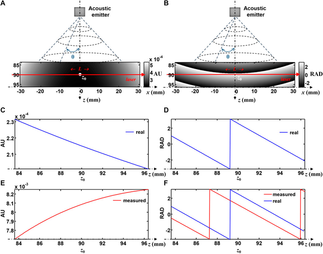
FIGURE 13. Schemes of the acoustic emitter, (A) scheme of the amplitude of the acoustic field, (B) scheme of the phase of the acoustic field, (C) amplitude profile along the z direction, (D) phase profile along the z direction, (E) amplitude profile of the integrated acoustic field along the laser beam, (F) phase profile of the integrated acoustic field along the laser beam (red line), comparison with the real phase profile (blue line).

So, Equations 10, 23 result from a “plane wave” consideration for the acoustic field. However, the transducer does not emit a plane wave because it is strongly divergent. The simulation shows that the further away from the acoustic source, the more the integrated amplitude deviates from the true amplitude. Thus, this probably explains the disagreement between interaction length estimation from holography and microphone measurements. It follows that the question of the conversion of the phase measurement into acoustic pressure remains open in the case of a non-plane acoustic field. The problem of quantitative measurement of the acoustic field by holography then remains to be investigated.

7 Conclusion

This paper presents the proof-of-concept for a simultaneous recording of multiple views for acoustic fields imaging. The principle is based on off-axis holography and spatial multiplexing of multi-wavelength holograms. Three wavelengths from three different laser lines are used to illuminate, at different incidence angles, the volume in which an acoustic wave propagates. The reference beams from the lasers are combined into a single three color beam and the spatial frequencies of the reference waves are adjusted so as to allow for the spatial multiplexing of digital holograms with the monochromatic sensor. After de-multiplexing and processing of the temporal sequence of digital color holograms, the amplitude and phase of the acoustic field along the views are obtained. The distortion of the acoustic amplitude is investigated with a theoretical modelling. Simulations permit to validate the modelling and the distortion rate can be estimated according to the experimental conditions. It follows that the distortion can be a posteriori compensated in order to get a correct amplitude measurement. The way to get quantitative acoustic pressure measurement is discussed according to realistic acoustic simulations and opens the way for future investigations. The first experimental results are presented for the case of the acoustic field emitted by an ultrasound transducer exited at the frequency of 40 kHz. Since the transducer does emit a spherical wave, the integrated amplitude along the laser beam deviates from the true amplitude. Thus, the question of the conversion of the holographic data into acoustic pressure is still open for free-field acoustic waves. This would open the way to quantitative holographic tomography of acoustic fields.

Data Availability Statement

Data underlying the results presented in this paper are not publicly available at this time but maybe obtained from Data underlying the results presented in this paper are not publicly available at this time but maybe obtained from the authors upon reasonable request.

Author Contributions

PP and KF directed the project. SH and PP prepared the theory and simulations. SH and PP performed the experiments. SH, KF, LB, and PP analyzed the experimental results. All authors contributed to the discussions and the preparation of the paper.

Conflict of Interest

The authors declare that the research was conducted in the absence of any commercial or financial relationships that could be construed as a potential conflict of interest.

Publisher’s Note

All claims expressed in this article are solely those of the authors and do not necessarily represent those of their affiliated organizations, or those of the publisher, the editors and the reviewers. Any product that may be evaluated in this article, or claim that may be made by its manufacturer, is not guaranteed or endorsed by the publisher.

Acknowledgments

The authors gratefully thank Guillaume Penelet from LAUM for very help-full discussions and recommendations. The authors thank the PROFAS B+ program for the scholarship provided to support the research program of Saoucene Hassad.

References

Bertling, K., Perchoux, J., Taimre, T., Malkin, R., Robert, D., Rakić, A. D., et al. (2014). Imaging of Acoustic Fields Using Optical Feedback Interferometry. Opt. Express 22, 30346–30356. doi:10.1364/oe.22.030346

PubMed Abstract | CrossRef Full Text | Google Scholar

Flanagan, J. L., Johnston, J. D., Zahn, R., and Elko, G. W. (1985). Computer‐steered Microphone Arrays for Sound Transduction in Large Rooms. J. Acoust. Soc. Am. 78, 1508–1518. doi:10.1121/1.392786

CrossRef Full Text | Google Scholar

Frank, S., and Schell, J. (2005). “Sound Field Simulation and Visualisation Based on Laser Doppler Vibrometer Measurements,” in Forum Acousticum. Budapest: EAA Events Proceedings, 91–97.

Google Scholar

Gong, L., Penelet, G., and Picart, P. (2018). Experimental and Theoretical Study of Density Fluctuations Near the Stack Ends of a Thermoacoustic Prime Mover. Int. J. Heat Mass Transf. 126, 580–590. doi:10.1016/j.ijheatmasstransfer.2018.05.027

CrossRef Full Text | Google Scholar

Gong, L., Penelet, G., and Picart, P. (2021). Noise and Bias in off-axis Digital Holography for Measurements in Acoustic Waveguides. Appl. Opt. 60, A93–A103. doi:10.1364/AO.404301

PubMed Abstract | CrossRef Full Text | Google Scholar

Groschup, R., and Grosse, C. (2015). Mems Microphone Array Sensor for Air-Coupled Impact-Echo. Sensors 15, 14932–14945. doi:10.3390/s150714932

PubMed Abstract | CrossRef Full Text | Google Scholar

Hafizovic, I., Nilsen, C.-I. C., Kjølerbakken, M., and Jahr, V. (2012). Design and Implementation of a Mems Microphone Array System for Real-Time Speech Acquisition. Appl. Acoust. 73, 132–143. doi:10.1016/j.apacoust.2011.07.009

CrossRef Full Text | Google Scholar

Hargather, M. J., Settles, G. S., and Madalis, M. J. (2010). Schlieren Imaging of Loud Sounds and Weak Shock Waves in Air Near the Limit of Visibility. Shock Waves 20, 9–17. doi:10.1007/s00193-009-0226-6

CrossRef Full Text | Google Scholar

Hashimoto, S., Takase, Y., Inoue, T., Nishio, K., Xia, P., Rajput, S. K., et al. (2022). Simultaneous Imaging of Sound Propagations and Spatial Distribution of Acoustic Frequencies. Appl. Opt. 61, B246–B254. doi:10.1364/ao.444760

PubMed Abstract | CrossRef Full Text | Google Scholar

Ishikawa, K., Tanigawa, R., Yatabe, K., Oikawa, Y., Onuma, T., and Niwa, H. (2018). Simultaneous Imaging of Flow and Sound Using High-Speed Parallel Phase-Shifting Interferometry. Opt. Lett. 43, 991–994. doi:10.1364/ol.43.000991

PubMed Abstract | CrossRef Full Text | Google Scholar

Ishikawa, K., Yatabe, K., Chitanont, N., Ikeda, Y., Oikawa, Y., Onuma, T., et al. (2016). High-speed Imaging of Sound Using Parallel Phase-Shifting Interferometry. Opt. Express 24, 12922–12932. doi:10.1364/oe.24.012922

PubMed Abstract | CrossRef Full Text | Google Scholar

Malkin, R., Todd, T., and Robert, D. (2014). A Simple Method for Quantitative Imaging of 2d Acoustic Fields Using Refracto-Vibrometry. J. Sound Vib. 333, 4473–4482. doi:10.1016/j.jsv.2014.04.049

CrossRef Full Text | Google Scholar

Matoba, O., Inokuchi, H., Nitta, K., and Awatsuji, Y. (2014). Optical Voice Recorder by off-axis Digital Holography. Opt. Lett. 39, 6549–6552. doi:10.1364/ol.39.006549

PubMed Abstract | CrossRef Full Text | Google Scholar

Merzkirch, W. (2012). Flow Visualization. New York: Academic Press.

Google Scholar

Oppenheim, A. V. (1999). Discrete-time Signal Processing. Pearson Education India.

Google Scholar

Ortiz, P. F. U., Perchoux, J., Arriaga, A. L., Jayat, F., and Bosch, T. (2018). Visualization of an Acoustic Stationary Wave by Optical Feedback Interferometry. Opt. Eng. 57, 051502. doi:10.1117/1.oe.57.5.051502

CrossRef Full Text | Google Scholar

Penelet, G., Leclercq, M., Wassereau, T., and Picart, P. (2016). Measurement of Density Fluctuations Using Digital Holographic Interferometry in a Standing Wave Thermoacoustic Oscillator. Exp. Therm. Fluid Sci. 70, 176–184. doi:10.1016/j.expthermflusci.2015.09.012

CrossRef Full Text | Google Scholar

P. Picart (Editor) (2015). New Techniques in Digital Holography (London : Hoboken, NJ: ISTE Ltd ; John Wiley & Sons, Inc). Instrumentation and measurement series.

Google Scholar

[Dataset] Pierce, A. D., and Beyer, R. T. (1990). Acoustics: An Introduction to its Physical Principles and Applications. 1989 edition. Acoustical Society of America.

Google Scholar

Rajput, S. K., Matoba, O., and Awatsuji, Y. (2018). Characteristics of Vibration Frequency Measurement Based on Sound Field Imaging by Digital Holography. OSA Contin. 1, 200–212. doi:10.1364/osac.1.000200

CrossRef Full Text | Google Scholar

Ramos Ruiz, A. E., Gürtler, J., Kuschmierz, R., and Czarske, J. W. (2019). Measurement of the Local Sound Pressure on a Bias-Flow Liner Using High-Speed Holography and Tomographic Reconstruction. IEEE Access 7, 153466–153474. doi:10.1109/access.2019.2948084

CrossRef Full Text | Google Scholar

Ren, F., Wang, Z., Qian, J., Liang, Y., Dang, S., Cai, Y., et al. (2019). Multi-view Object Topography Measurement with Optical Sectioning Structured Illumination Microscopy. Appl. Opt. 58, 6288–6294. doi:10.1364/ao.58.006288

PubMed Abstract | CrossRef Full Text | Google Scholar

Schnars, U., and Jüptner, W. (1994). Direct Recording of Holograms by a CCD Target and Numerical Reconstruction. Appl. Opt. 33, 179–181. doi:10.1364/AO.33.000179

PubMed Abstract | CrossRef Full Text | Google Scholar

Seo, Y.-H., Choi, H.-J., Bae, J.-W., Kang, H.-J., Lee, S.-H., Yoo, J.-S., et al. (2007). A New Coding Technique for Digital Holographic Video Using Multi-View Prediction. IEICE Trans. Inf. Syst. E90-D, 118–125. doi:10.1093/ietisy/e90-1.1.118

CrossRef Full Text | Google Scholar

Shaked, N. T., Rinehart, M. T., and Wax, A. (2009). Dual-interference-channel Quantitative-phase Microscopy of Live Cell Dynamics. Opt. Lett. 34, 767–769. doi:10.1364/OL.34.000767

PubMed Abstract | CrossRef Full Text | Google Scholar

Shimobaba, T., Masuda, N., Ichihashi, Y., and Ito, T. (2010). Real-time Digital Holographic Microscopy Observable in Multi-View and Multi-Resolution. J. Opt. 12, 065402. doi:10.1088/2040-8978/12/6/065402

CrossRef Full Text | Google Scholar

Takaki, Y. (2015). Super Multi-View and Holographic Displays Using Mems Devices. Displays 37, 19–24. doi:10.1016/j.displa.2014.09.002

CrossRef Full Text | Google Scholar

Takase, Y., Shimizu, K., Mochida, S., Inoue, T., Nishio, K., Rajput, S. K., et al. (2021). High-speed Imaging of the Sound Field by Parallel Phase-Shifting Digital Holography. Appl. Opt. 60, A179–A187. doi:10.1364/ao.404140

PubMed Abstract | CrossRef Full Text | Google Scholar

Torras-Rosell, A., Barrera-Figueroa, S., and Jacobsen, F. (2012). Sound Field Reconstruction Using Acousto-Optic Tomography. J. Acoust. Soc. Am. 131, 3786–3793. doi:10.1121/1.3695394

PubMed Abstract | CrossRef Full Text | Google Scholar

Yamaguchi, I., Matsumura, T., and Kato, J.-i. (2002). Phase-shifting Color Digital Holography. Opt. Lett. 27, 1108–1110. doi:10.1364/OL.27.001108

PubMed Abstract | CrossRef Full Text | Google Scholar

Yamaguchi, I., and Zhang, T. (1997). Phase-shifting Digital Holography. Opt. Lett. 22, 1268. doi:10.1364/OL.22.001268

PubMed Abstract | CrossRef Full Text | Google Scholar