- 1Department of Ophthalmology, Hallym University, Dongtan Sacred Heart Hospital, Hwaseong-si, South Korea
- 2Department of Environmental Engineering, Inha University, Incheon, South Korea
- 3Department of Industrial and Management Engineering, Myongji University, Yongin-si, South Korea
- 4Department of Ophthalmology and Visual Science, Catholic University of Korea, Seoul St. Mary's Hospital, Seoul, South Korea
Ozone (O3) is a commonly known air pollutant that causes adverse health effects. This study developed a multi-level prediction model for conjunctivitis in outpatients due to exposure to O3 by using 3 years of ambient O3 data, meteorological data, and hospital data in Seoul, South Korea. We confirmed that the rate of conjunctivitis in outpatients (conjunctivitis outpatient rate) was highly correlated with O3 (R2 = 0.49), temperature (R2 = 0.72), and relative humidity (R2 = 0.29). A multi-level regression model for the conjunctivitis outpatient rate was well-developed, on the basis of sex and age, by adding statistical factors. This model will contribute to the prediction of conjunctivitis outpatient rate for each sex and age, using O3 and meteorological data.
Introduction
Air pollution is a significant global issue that has substantial effects on air quality, human health, earth hydrological cycle, and climate change (Correia et al., 2013; Lelieveld et al., 2015; Sicard et al., 2016; Duan et al., 2017). The Clean Air Act recommends that the U.S. Environmental Protection Agency (EPA) build National Ambient Air Quality Standards for “six criteria air pollutants,” which include particulate matter (PM), carbon monoxide (CO), sulfur dioxide (SO2), nitrogen dioxide (NO2), lead, and ozone (O3) (U. S. Environmental Protection Agency, 2010). The six criteria air pollutants are known to cause a wide range of health effects, including respiratory (Guan et al., 2016), cardiovascular (Franklin et al., 2015), eye (Szyszkowicz et al., 2018), and skin diseases (Eastham et al., 2018). Among the six criteria air pollutants, O3 is commonly known as the most toxic component produced by photochemical reactions in the atmosphere (Seinfeld and Pandis, 2006). Bell et al. (2004) revealed the relationship between O3 and short-term mortality in 95 communities in the United States.
Previous epidemiological studies have associated significant adverse human health effects by exposure to O3 (Fann et al., 2012). While much attention is focused on the effect of O3 on respiratory diseases (Sousa et al., 2013; Karakatsani et al., 2017; Stergiopoulou et al., 2018), less effort has been attached to discerning its role in eye disease. The effects of O3 on eye disease have been investigated in epidemiological studies (Hong et al., 2016; Hwang et al., 2016). Hong et al. (2016) studied the relationships of air pollutants (SO2, NO2, O3, PM10, PM2.5) and meteorological data with allergic conjunctivitis outpatients by using a retrospective registry study. However, that study had limitations in its analysis of the multi-level effect of air pollutants and meteorological data on conjunctivitis outpatient rate because it used the relationships between outpatients and individual factors. Hwang et al. found that dry eye disease outpatient rate was associated with high ozone concentration and low relative humidity, by using multivariable regression analysis.
The goal of this study was to develop a multi-level prediction model for conjunctivitis outpatient rate according to O3 and meteorological factors in Seoul, South Korea. Three years of O3 data, meteorological factors, and conjunctivitis outpatient rates in Seoul are reported. The subsequent discussion focuses on development and validation of a conjunctivitis outpatient prediction model with those data.
Materials and Methods
Hospitalization Data
Conjunctivitis outpatient statistic data between January 1, 2011 and December 31, 2013 in Seoul were obtained from the Korea Health Insurance Review and Assessment Service (KHIRAS) for research purpose. The KHIRAS provided number of ophthalmology outpatient based on diagnostic codes excluding patient personal information. In total, 97.2% of Korean residents receive Korea National Health Insurance Service (KNHIS) health insurance (Korean National Health Insurance Services, 2016). All hospitals in Korea are required to submit claim documents for medical services. We obtained data for 48,344 conjunctivitis patients, except waterborne and chronic conjunctivitis patients, based on disease code. The conjunctivitis outpatient rates of each age range and gender were calculated as the number of outpatients divided by the population, in order to normalize the data.
Air Pollutants and Meteorological Data
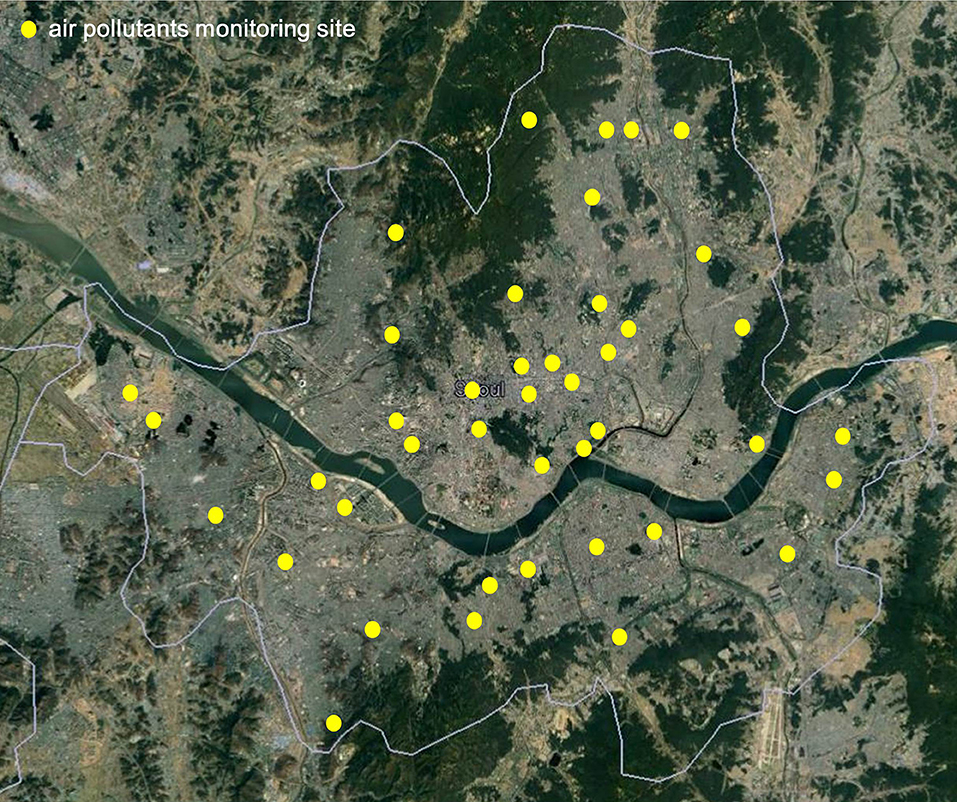
Hourly measurements of O3 were obtained for the years between January 1, 2011 and December 31, 2013 from 40 ground-based air pollutant monitoring sites operated by the city of Seoul, South Korea (Figure 1). To determine how meteorological factors are related to conjunctivitis outpatient rate, hourly temperature and relative humidity data were obtained at the collocated sites. We used weekly average data of patient visits and meteorological factors to avoid statistical errors due to no patient visits on weekends.
Model Development
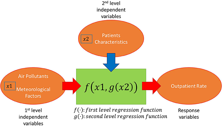
A multi-level regression model (two-level regression model) was developed for the prediction of conjunctivitis outpatient rate. The structure of the model is shown in Figure 2. The level 1 regression model describes the relationship between level 1 independent variables and the conjunctivitis outpatient rate. Four air pollutants (PM10, NO2, SO2, and O3) and two meteorological factors (temperature and humidity) were considered as candidate level 1 model independent variables. Correlations between these factors and the conjunctivitis outpatient rate were calculated. PM10, NO2, and SO2 were removed from the level 1 regression model due to their negative correlations. The level 1 regression model was developed for each age range and gender. The shapes of the level 1 regression model were changed based on age range and gender. The coefficients of level 1 regression model can be explained by level 2 independent variables. An ANOVA was tested for the level 1 regression models and multi-level regression models. The detailed analysis and results are shown in the next section.
Results and Discussion
Figure 3 shows the weekly trends of meteorological factors, O3, and conjunctivitis outpatient rates between 2011 and 2013. The highest and lowest seasonal averages of O3 concentrations from the sampling sites were 0.27 (April–June) and 0.12 ppm (October–December), respectively. The July–September data contained the highest values for temperature (24.7°C), humidity (70.7%), and number of conjunctivitis outpatients (359.5), while between January and March data had lowest values for temperature (−0.8°C), humidity (51.2%), and number of conjunctivitis outpatients (267.0). The number of conjunctivitis outpatients was positively correlated with the temperature (R2 = 0.72) and humidity (R2 = 0.29). The correlation coefficient between the number of conjunctivitis outpatients and O3 is 0.49. We developed a regression model based on the relationships between the number of conjunctivitis outpatients and other factors.
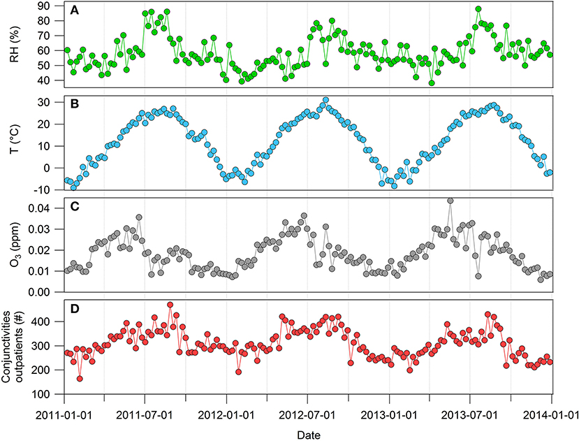
Figure 3. Weekly trends of (A) relative humidity (RH), (B) temperature (T), (C) O3, and (D) number of conjunctivitis outpatients.
In previous research (Hong et al., 2016), the effect of each factor on conjunctivitis was examined individually. In contrast, in this study, regression models were developed with five independent factors, including temperature, humidity, O3, sex, and age, in order to consider these factors concurrently. First, the regression models for temperature, humidity, and O3 were developed, then sex and age factors were added by multi-level regression modeling. All regression models were developed by R 3.2.3 with the MASS library. The response variable and independent variables for the developed regression models were as follows:
y: outpatient rate per week (the number of outpatients per week/the population),
X1: average temperature per week + 20 (°C),
X2: average humidity per week (%),
X3: average O3 per week(ppm).
y is the response variable of the developed regression models; X1, X2, and X3 are the independent variables. In order to prevent negative values, the average temperature per week + 20 was used for X1, instead of the average temperature. Three simple regression models were developed, including the linear, linear + log, and linear + exponential models, with these response variable and independent variables (Kutner et al., 2004). The models are shown below:
Model 1: y = β0 + β11X1 + β21X2 + β31X3 + ε,
Model 2: y = β0 + β11X1 + β12ln(X1) + β21X2 + β22ln(X2) + β31X3 + β32ln(X3) + ε,
Model 3: y = β0 + β11X1 + β12exp(X1) + β21X2 + β22exp(X2) + β31X3 + β32exp(X3) + ε.
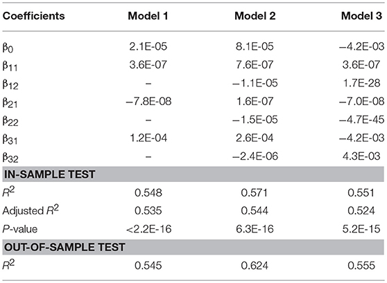
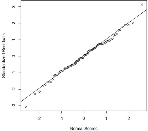
The estimated coefficients of each model and the test results are shown in Table 1. One week for every 3 weeks over 156 weeks was randomly selected for only model validation (out-of-sample test). The other 2 weeks for every 3 weeks were used for model development and validation (in-sample test). All three models were significant based on their small p values. However, model 2 was the best model due to better R2 and Adjusted R2 for in-sample and out-of-sample tests. Figure 4 shows the normal probability plot for model 2. Most residuals in the graph are located near the diagonal line, which shows normality of residuals.
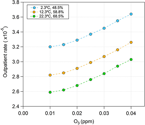
The model 2 can predict the outpatient rate with temperature, humidity, and O3. The out of sample test shows the prediction accuracy of the regression model since the sample for out of sample test does not use for model development. The Figure 5 shows an example of the outpatient rate prediction with the model 2. Figure 5 shows the estimated outpatient rate by model 2 for three different temperature and humidity combinations (Temperature, Humidity) over O3. In South Korea, temperature and humidity increase during the summer and decrease during the winter. The three temperature and humidity combinations, high, average, and low, were determined based on the average temperature and humidity over the test time periods; these were 12.34°C and 58.5%, respectively. The outpatient rate increased with increased temperature and humidity. In contrast, the dry eye disease outpatient rate increased with reduced relative humidity (Hwang et al., 2016). This is presumably due to multiple factors rather than the simple effect of relative humidity. The regression models including sex and age, were developed based on model 2. The additional independent variables for the regression model were defined as follows:
Sex: 0 for male and 1 for female,
Age: 1 (0–9 years old), 2 (10–19 years old), 3 (20–29 years old), …, 9 (> 80 years old).
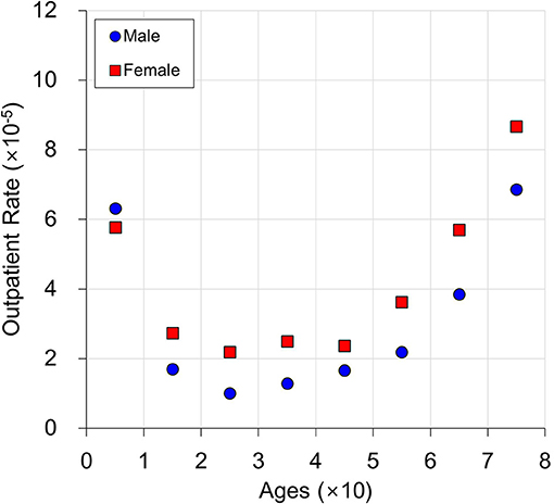
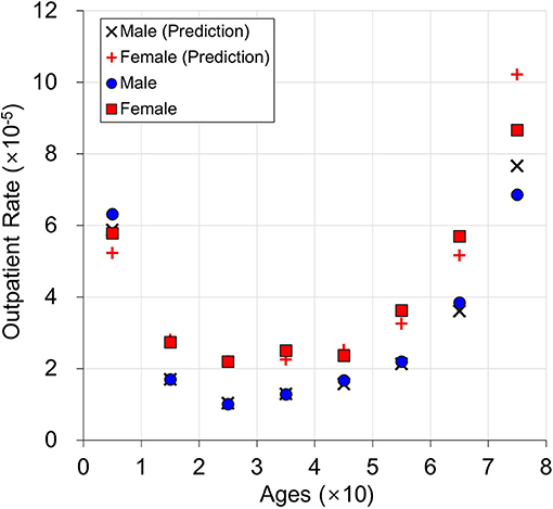
Figure 6 shows the average outpatient rate over 156 weeks for each sex and age. The outpatient rates decrease until the 20–29 years old group, then typically increase for the younger ages for both males and females. The female outpatient rates are higher than those for males, for all age ranges except 0–9 years old.
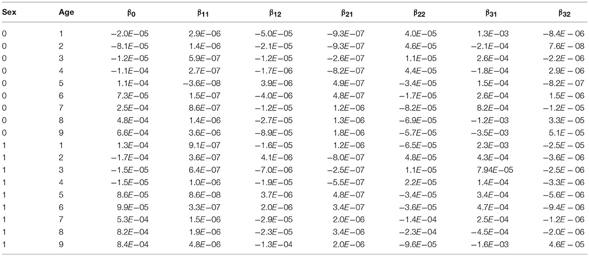
Regression models were developed for each sex and age combination, as shown in Table 2. However, sex and age can be independent variables by assuming each coefficient of model 2 is a function of sex and age.
Assuming β0 and βij in Table 2 are functions of sex and age, then let the function be g0(sex, age) and gij(sex, age); the regression model can be represented as follows:
This is a multi-level regression model; thus, model 2 is a first-level regression model and g0(sex, age) and gij (sex, age) are second-level regression models (Gelman and Hill, 2007). This model is applicable when there is a hierarchical structure among independent variables. In this study, sex and age were considered higher-level independent variables. Because the effect of age is nonlinear, as shown in Figure 6, the regression model for g0(sex, age) was developed by the following relationship: sex + age + sex · age + ln (age) + sex· ln (age) + exp(age) + sex · exp(age). In order to develop a simple model, the model selected for gij (sex, age) was one of the following relationships:
1) sex + age + sex · age,
2) sex + ln(age) + sex · ln(age),
3) sex + exp(age) + sex · exp(age).
The model that provided the highest R2 value in Table 2, when βij was the response variable and sex and age were the independent variables, was selected. Two regression models were separately developed by age, because the effect of age dramatically changed between 20 and 30 years old, as shown in Figure 6. The first regression model for ages 1 and 2 is as follows (this model does not have any ln(age) and exp(age) because age has only two levels):
The second regression model for ages 3, 4, 5, 6, and 7 is as follows (Age 8 and 9 data were removed for model development because their data patterns differ from the others, likely due to the effects of old age):
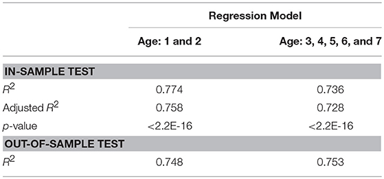
Table 3 shows the test results for the two developed regression models. The p values for both regression models were less than 2.2e-16; both models were statistically significant. In the in-sample tests, when ages were 1 and 2, R2 and adjusted R2 were 0.774 and 0.758, respectively. When ages were 3 through 7, R2 and adjusted R2 were 0.736 and 0.728, respectively. In the out-of-sample tests, when age was 1 and 2, R2 was 0.7; when age was 3 through 7, R2 was 0.753. This result shows that the model is valid. It is also possible to develop multi-level regression models with model 1 or model 3 in Table 1; these provide lower R2 than those by model 2. The regression models can predict conjunctivitis outpatient rate and perform sensitivity analysis for each independent variable. To predict the conjunctivitis outpatient rate by sex and age, model 1 can be used. Model 3 can be used to predict the conjunctivitis outpatient rate by temperature, humidity, and O3. Model 2, the multi-regression model, can be applied when all independent variables are combined to predict conjunctivitis outpatient rate.
An example of multi-level regression model prediction is shown in Figure 7. The average temperature, average humidity, and average O3 (0.018 ppm) over 156 weeks were used for this graph. This is compared with the average outpatient rate in Figure 6. The average outpatient rates are close to predictions by the multi-level regression model. When age is 1, the male outpatient rate is higher than the female outpatient rate. In contrast, in all other age ranges, male outpatient rates are lower than female outpatient rates. The multi-regression model predicts the number of conjunctivitis outpatients based on age and sex, by using the weekly average temperature, humidity, and O3.
Figure 8 shows the comparison between prediction and actual outpatient rate by using out-of-sample tests. Fifty-two-week data for each sex and age were used for all 3 years. The overall prediction followed the individual trends, except for a large variation within age 7; this is presumably related to increased mortality in the age 7 group. These results indicate that the developed multi-regression model can predict the incidence of conjunctivitis by using age, sex, temperature, humidity, and O3. The level 1 regression model can predict the overall incidence of conjunctivitis without consideration of sex and age (Model 2 in Table 2).
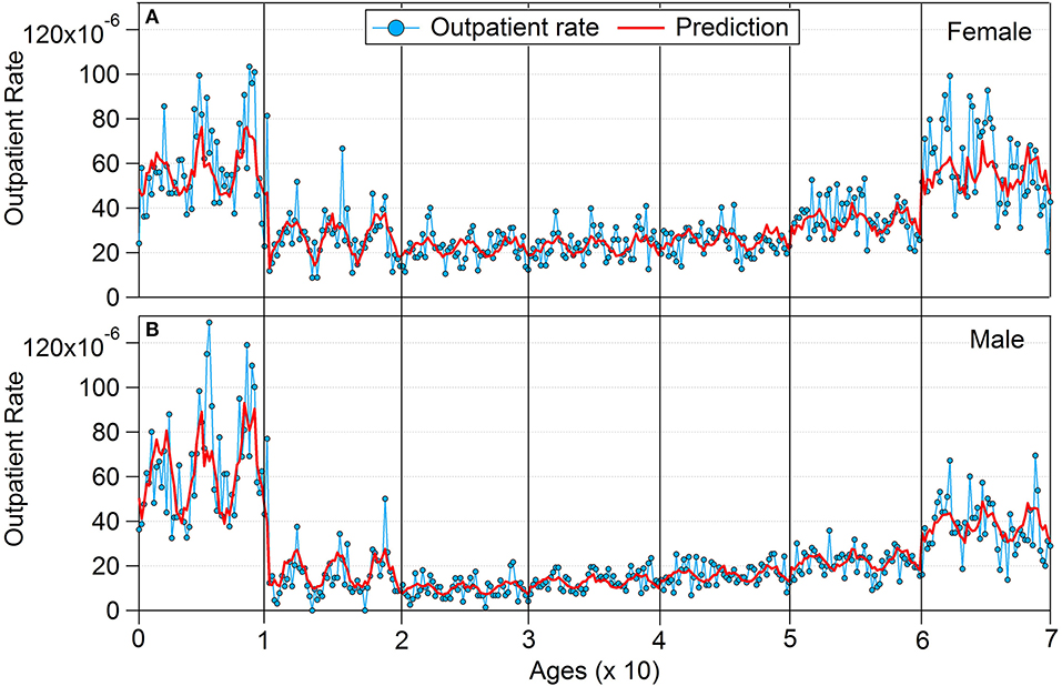
Figure 8. Prediction and actual outpatient rate using out-of-sample testing: (A) female and (B) male.
May insert up to 5 heading levels into your manuscript as can be seen in “Styles” tab of this template. These formatting styles are meant as a guide, as long as the heading levels are clear, Frontiers style will be applied during typesetting.
Conclusions
The weekly average O3 concentrations were highly correlated with meteorological factors and numbers of outpatients. This study provides models for prediction of conjunctivitis outpatient rates by using multiple concurrent independent variables, such as temperature, humidity, and O3. This model verifies the effect of O3 by the developed regression model. When O3 increases, the outpatient rate also increases. A method to develop a multi-level regression model for the conjunctivitis outpatient rate is provided. Sex and age factors are added to the developed regression model by using multi-level regression modeling. This enabled us to predict the conjunctivitis outpatient rate by using five independent factors concurrently. The developed models can be used to identify the characteristics of conjunctivitis outpatient rate on the basis of each independent variable. Test results for the developed models and their prediction examples are provided. Other pollutants can be included in future research. In future study, we will apply the multi-level regression model to other environmental diseases.
Author Contributions
SP and C-KJ supervised overall research. J-WS contributed to paper writing and model development. J-SY performed the air pollutant and meteorological data analysis.
Funding
This study was funded by the Korea Ministry of Environment (MOE), as the Environmental Health Action Program (2016001360005).
Conflict of Interest Statement
The authors declare that the research was conducted in the absence of any commercial or financial relationships that could be construed as a potential conflict of interest.
References
Bell, M. L., McDermott, A., Zeger, S. L., Samet, J. M., and Dominici, F. (2004). Ozone and short-term mortality in 95 US urban communities, 1987-2000. J. Am. Med. Assoc. 292, 2372–2378. doi: 10.1001/jama.292.19.2372
Correia, A. W., Pope, C. A., Dockery, D. W., Wang, Y., Ezzati, M., and Dominici, F. (2013). The effect of air pollution control on life expectancy in the United States: an analysis of 545 US counties for the period 2000 to 2007. Epidemiology 24, 23–31. doi: 10.1097/EDE.0b013e3182770237
Duan, K., Sun, G., Zhang, Y., Yahya, K., Wang, K., Madden, J. M., et al. (2017). Impact of air pollution induced climate change on water availability and ecosystem productivity in the conterminous United States. Clim. Change 140, 259–272. doi: 10.1007/s10584-016-1850-7
Eastham, S. D., Keith, D. W., and Barrett, S. R. H. (2018). Mortality tradeoff between air quality and skin cancer from changes in stratospheric ozone. Environ. Res. Lett. 13:34035. doi: 10.1088/1748-9326/aaad2e
Fann, N., Lamson, A. D., Anenberg, S. C., Wesson, K., Risley, D., and Hubbell, B. J. (2012). Estimating the national public health burden associated with exposure to ambient PM2.5 and ozone. Risk Anal. 32, 81–95. doi: 10.1111/j.1539-6924.2011.01630.x
Franklin, B. A., Brook, R., and Arden Pope, C. (2015). Air pollution and cardiovascular disease. Curr. Probl. Cardiol. 40, 207–238. doi: 10.1016/j.cpcardiol.2015.01.003
Gelman, A., and Hill, J. (2007). Data Analysis Using Regression and Multilevel/Hierarchical Models. Cambridge: Cambridge University press.
Guan, W.-J., Zheng, X.-Y., Chung, K. F., and Zhong, N.-S. (2016). Impact of air pollution on the burden of chronic respiratory diseases in China: time for urgent action. Lancet 388, 1939–1951. doi: 10.1016/S0140-6736(16)31597-5
Hong, J., Zhong, T., Li, H., Xu, J., Ye, X., Mu, Z., et al. (2016). Ambient air pollution, weather changes, and outpatient visits for allergic conjunctivitis: a retrospective registry study. Sci. Rep. 6:23858. doi: 10.1038/srep23858
Hwang, S. H., Choi, Y.-H., Paik, H. J., Wee, W. R., Kim, M. K., and Kim, D. H. (2016). Potential importance of ozone in the association between outdoor air pollution and dry eye disease in South Korea. JAMA Ophthalmol. 134:503. doi: 10.1001/jamaophthalmol.2016.0139
Karakatsani, A., Samoli, E., Rodopoulou, S., Dimakopoulou, K., Papakosta, D., Spyratos, D., et al. (2017). Weekly personal ozone exposure and respiratory health in a panel of Greek schoolchildren. Environ. Health Perspect. 125:077016. doi: 10.1289/EHP635
Korean National Health Insurance Services (2016). Key Statistics of National Health Insurance. Available online at: http://www.nhis.or.kr/menu/boardRetriveMenuSet.xx?menuId=F3322
Kutner, M. H., Nachtsheim, C. J. J., Neter, J., and Li, W. (2004). Applied Linear Statistical Models. New York, NY: McGraw-Hill/Irwin.
Lelieveld, J., Evans, J. S., Fnais, M., Giannadaki, D., and Pozzer, A. (2015). The contribution of outdoor air pollution sources to premature mortality on a global scale. Nature 525, 367–371. doi: 10.1038/nature15371
Seinfeld, J. H., and Pandis, S. N. (2006). Atmospheric Chemistry and Physics: From Air Pollution to Climate Change. Hoboken, NJ: John Wiley & Sons.
Sicard, P., Augustaitis, A., Belyazid, S., Calfapietra, C., de Marco, A., Fenn, M., et al. (2016). Global topics and novel approaches in the study of air pollution, climate change and forest ecosystems. Environ. Pollut. 213, 977–987. doi: 10.1016/j.envpol.2016.01.075
Sousa, S. I. V., Alvim-Ferraz, M. C. M., and Martins, F. G. (2013). Health effects of ozone focusing on childhood asthma: what is now known - a review from an epidemiological point of view. Chemosphere 90, 2051–2058. doi: 10.1016/j.chemosphere.2012.10.063
Stergiopoulou, A., Katavoutas, G., Samoli, E., Dimakopoulou, K., Papageorgiou, I., Karagianni, P., et al. (2018). Assessing the associations of daily respiratory symptoms and lung function in schoolchildren using an Air Quality Index for ozone: results from the RESPOZE panel study in Athens, Greece. Sci. Total Environ. 633, 492–499. doi: 10.1016/j.scitotenv.2018.03.159
Szyszkowicz, M., Kousha, T., Castner, J., and Dales, R. (2018). Air pollution and emergency department visits for respiratory diseases: a multi-city case crossover study. Environ. Res. 163, 263–269. doi: 10.1016/j.envres.2018.01.043
U. S. Environmental Protection Agency (2010). National Ambient Air Quality Standards (NAAQS). Available online at: http://www.epa.gov/air/criteria.html
Keywords: multi-level, conjunctivitis, ozone, prediction model, meteorology
Citation: Seo J-W, Youn J-S, Park S and Joo C-K (2018) Development of a Conjunctivitis Outpatient Rate Prediction Model Incorporating Ambient Ozone and Meteorological Factors in South Korea. Front. Pharmacol. 9:1135. doi: 10.3389/fphar.2018.01135
Received: 28 August 2018; Accepted: 18 September 2018;
Published: 09 October 2018.
Edited by:
Vivek K. Bajpai, Dongguk University Seoul, South KoreaReviewed by:
Tri Khoa Nguyen, University of Ulsan, South KoreaYoung-Min Kim, Hallym University, South Korea
Thach Duy Phan, École Polytechnique de Montréal, Canada
Copyright © 2018 Seo, Youn, Park and Joo. This is an open-access article distributed under the terms of the Creative Commons Attribution License (CC BY). The use, distribution or reproduction in other forums is permitted, provided the original author(s) and the copyright owner(s) are credited and that the original publication in this journal is cited, in accordance with accepted academic practice. No use, distribution or reproduction is permitted which does not comply with these terms.
*Correspondence: SeJoon Park, c29ubXVwc2pAbWp1LmFjLmty
Choun-Ki Joo, Y2tqb29AY2F0aG9saWMuYWMua3I=
 Jeong-Won Seo1
 Jong-Sang Youn
 SeJoon Park