Leveraging design of experiments to build chemometric models for the quantification of uranium (VI) and HNO3 by Raman spectroscopy

Partial least squares regression (PLSR) and support vector regression (SVR) models were optimized for the quantification of U(VI) (10–320 g L⁻¹) and HNO₃ (0.6–6 M) by Raman spectroscopy with optimized calibration sets chosen by optimal design of experiments. The designed approach effectively minimized the number of samples in the calibration set for PLSR and SVR by selecting sample concentrations with a quadratic process model, despite complex confounding and covarying spectral features in the spectra. The top PLS2 model resulted in percent root mean square errors of prediction for U(VI), HNO₃, and NO₃⁻ of 3.7%, 3.6%, and 2.9%, respectively. PLS1 models performed similarly despite modeling an analyte with a majority linear response (i.e., uranyl symmetric stretch) and another with more covarying vibrational modes (i.e., HNO₃). Partial least squares (PLS) model loadings and regression coefficients were evaluated to better understand the relationship between weaker Raman bands and covarying spectral features. Support vector machine models outperformed PLS1 models, resulting in percent root mean square error of prediction values for U(VI) and HNO₃ of 1.5% and 3.1%, respectively. The optimal nonlinear SVR model was trained using a similar number of samples (11) compared with the PLSR model, even though PLS is a linear modeling approach. The generic D-optimal design presented in this work provides a robust statistical framework for selecting training set samples in disparate two-factor systems. This approach reinforces Raman spectroscopy for the quantification of species relevant to the nuclear fuel cycle and provides a robust chemometric modeling approach to bolster online monitoring in challenging process environments.

1 Introduction

Online monitoring techniques have been investigated for process monitoring applications in the nuclear field for many decades via direct techniques (e.g., spectrophotometry) and physiochemical measurements (e.g., density) (Bryan et al., 2011; Kirsanov et al., 2017; Colle et al., 2020). These methods can characterize multiple species simultaneously and yield information within seconds to minutes (Kirsanov et al., 2017; Lascola et al., 2017; Lines et al., 2020; Sadergaski et al., 2020; Sadergaski et al., 2022a). Rapid, in-line quantification provides numerous operational benefits for processes commonly taking place in harsh, restrictive, and expensive working environments such as hot cells. Identifying deviations from normal operations in nuclear facilities is important for many reasons such as controlling processing streams for efficient radiochemical separations and monitoring diversions for proliferation and safeguards purposes.

Ultraviolet–visible–near-infrared spectrophotometry has been used since the 1970s for the quantification of actinide and HNO₃ concentrations and metal ion speciation (Burck, 1992). Raman spectroscopy is also useful for actinide measurements, particularly actinyl ions, including U(VI), Np(V), Np(VI), and Pu(VI), which have Raman-active vibrational modes (Guillaume et al., 1982; Felmy et al., 2023). For trace U(VI), time-resolved laser-induced fluorescence can be used to quantify concentration and determine speciation (Matusi et al., 1988; Moulin et al., 1994; Couston et al., 1995; Moulin et al., 1996; Sadergaski and Andrews, 2022; Sadergaski et al., 2024). With increasing HNO₃ concentration, UO₂²⁺ hydrate complexes are replaced by coordinating nitrate ions (NO₃⁻) to form U(NO₃)⁺, U(NO₃)₂, and even U(NO₃)₃⁻, which produce unique spectral features, particularly in electronic spectroscopy (Burck, 1992; Ikeda-Ohno et al., 2009).

Optical spectra collected in challenging process media over a wide range of conditions are often best modeled using multivariate analysis or chemometrics (Pelletier, 2003; Casella et al., 2013; Sadergaski et al., 2022b). Areas where chemometrics have been most successful include multivariate calibration, pattern recognition, classification, multivariate processing monitoring, and others (Wold and Sjostrom, 1998). A well-established supervised chemometric method is partial least squares regression (PLSR), which is a factor analysis method that models entire spectra to find the structure in X (i.e., spectral matrix) that is most predictive for Y matrix (i.e., concentration matrix) (Wold et al., 2001).

Although this supervised chemometric approach is very powerful, it normally depends on collecting a spectral dataset representative of the anticipated process conditions. It can be challenging to produce these training sets in the nuclear field because radioactive materials are in short supply or difficult to handle. Design of experiments (e.g., optimum designs) can be used to minimize the number of samples in a training set without sacrificing predictive capabilities to minimize time and waste compared with more traditional methods (Czitrom, 1999; Wold et al., 2003; Guo et al., 2021). The primary goal is generating a balanced sample distribution in each direction of the design space to ensure all points have reasonable influence on the solution (i.e., PLSR model). However, the relationship between the designed concentration matrix and PLSR prediction performance is somewhat empirical because optimal design only considers Y, while a PLSR model correlates both spectra (X matrix) and response variable(s) (i.e., Y matrix). Additionally, most examples of this method are not generalized and are often applied to relatively simple systems with little covariance or confounding spectral features (Bondi et al., 2012; Steinbach et al., 2017; Sadergaski et al., 2022b; Sadergaski et al., 2023).

This study minimized the number of calibration set samples using a two-factor D-optimal design for the quantification of U(VI) (10–320 g/L) and HNO₃ (0.6–6 M) while optimizing PLSR prediction performance to bolster the monitoring approach for nuclear fuel cycle applications (Burns and Moyer, 2016; Einkauf and Burns, 2020). The generic two-factor D-optimal design can be extended to numerous systems by simply scaling the endpoints to provide a more balanced estimate of model parameters. Additionally, the performance of the linear PLSR model was compared with nonlinear support vector regression (SVR), which is a type of support vector machine (SVM) useful for regression tasks (Deiss et al., 2020; Rodriguez-Perez and Bajorath, 2022). Very few studies have evaluated the effect of training set size and composition on SVM modeling (Rodriguez-Perez et al., 2017). The scientific advancements in this work are threefold; this study 1) established a generalized D-optimal design for optimizing training set sample compositions in linear PLSR and nonlinear SVR models, 2) demonstrated a consistent designed approach amenable to both simple and more complex systems with collinear and covarying spectral features, and 3) compared the prediction performance of more traditional PLSR and nonlinear SVR models. These findings further establish the optical spectroscopy and chemometric methods for online monitoring applications within and beyond the nuclear field.

2 Methods

All chemicals were commercially obtained (American Chemical Society grade) and used as received unless otherwise stated. Concentrated HNO₃ (70%) was purchased from Sigma-Aldrich. Certified 10,000 μg mL⁻¹ U (²³⁸U, depleted) was purchased from SPEX CertiPrep. Samples were prepared using deionized water with MilliporeSigma Milli-Q purity (18.2 MΩ∙cm at 25°C). Uranyl nitrate hexahydrate (UNH) crystals were purchased from International Bio-Analytical Industries and purified by crystallization.

2.1 Sample preparation

Calibration samples (16) contained U (VI) (10–320 g L⁻¹ U) and HNO₃ (0.6–6 M) to cover the anticipated solution conditions, and several validation samples (27) were within and slightly beyond this range (Supplementary Tables S1, S2). Samples were prepared with volumetric flasks and pipettes and gravimetrically measured using a Mettler Toledo model XS204 balance with an accuracy of ±0.0001 g. A U stock concentration at 533 g L⁻¹ U was prepared by dissolving UNH crystals in 0.01 M HNO₃. The concentration of the U(VI) stock solution was checked by diluting an aliquot for spectrophotometry (QEPro by Ocean Insight) using a molar extinction coefficient of 7.7 M⁻¹cm⁻¹ for the 415 nm absorption peak. The molar extinction coefficient was determined by analyzing a 10,000 ppm inductively coupled plasma optical emission spectroscopy stock solution in 5% HNO₃ with a 1 cm quartz cuvette.

2.2 Vibrational spectroscopy

An imaging iHR320 spectrometer (Horiba Scientific), a continuous-wave CNI 532 nm laser operating at 150 mW, and a general-purpose reflection probe (Spectra Solutions Inc.) were used to collect Stokes Raman spectra. Two multimode fibers—a 105 µm core diameter fiber and a 400 µm core diameter fiber—were used on the excitation and emission side, respectively. Triplicate spectra were recorded from 200 to 4,000 cm⁻¹ using a grating with 600 grooves per millimeter, a 100 µm slit size, a 0.5 s integration time, and four accumulations. Each spectrum was processed using LabSpec 6 software (Horiba Scientific). Static liquid samples were analyzed in 1.8 mL borosilicate glass vials with a threaded cap and using a sample/Raman probe holder made by Spectra Solutions Inc.

2.3 Design of experiments

Experimental designs were built using Design-Expert (v.22.0.5) by Stat-Ease Inc. D-optimal designs select sample concentrations by iteratively minimizing the determinant of the variance-covariance matrix. The U(VI) and HNO₃ are referred to as factors, and particular concentrations are levels. A run refers to a single sample, and the sample size is the total number of runs in the experiment. The design was generated for two continuous levels 1–10 using a quadratic process model and contained six required model points and an additional 10 lack-of-fit (LOF) points (Supplementary Table S3). Five LOF points were needed to achieve a fraction of design space near one (0.98) calculated by mean error type, δ = 2, σ = 1, and α = 0.05, which indicates good prediction capability over the factor range (Zahran et al., 2003). The variable δ describes the maximum acceptable half-width (i.e., margin of error), σ is an estimate of the standard deviation, and α is the significance level used in the statistical analysis. If additional LOF points were needed, it would suggest that a higher-order model should be used.

2.4 Multivariate analysis and preprocessing

The Vektor Direktor v2.0 software by the KAX Group was used to build PLSR/SVR models and for data preprocessing. Cross validation (CV) was used to determine the optimal number of latent variables (LVs) to include in the model as the LV with the last significant decrease in root mean square error (RMSE) of CV (RMSECV). PLSR models were built with one Y variable (PLS1) and multiple Y variables (PLS2) to compare performance. PLS2 models are typically better at accounting for covariance or multicollinearity in the spectral dataset. On the other hand, PLS1 models can be tailored to the spectral features of each species, which may require unique combinations of preprocessing and feature selection strategies. A full leave-one-out CV was used for PLSR and SVR models. This is performed by randomly leaving one sample out of the calibration set until every sample is left out once and recalibrating sub-models on the remaining data. Spectra were mean-centered prior to analysis unless otherwise stated.

Spectral data were preprocessed prior to modeling. Preprocessing strategies can account for artifacts (e.g., baseline shifts) that are expected in monitoring applications and optimize the regression. A simple baseline offset was used to subtract a slightly increased baseline at higher U(VI) concentrations. Standard normal variate (SNV) is one of the most common scatter correction algorithms and only uses data within each individual spectrum to center and scale the data (Supplementary Figure S1). Savitsky–Golay first derivatives were tested but did not improve the models. Spectra were trimmed to evaluate how different regions of the spectra affected model performance.

The SVM algorithm is a widely used machine learning method for classification, ranking, multiclass prediction, and regression modeling (Rodriguez-Perez and Bajorath, 2022). The SVM approach was introduced decades ago and was originally designed for binary object classification. SVMs find a hyperplane in a high dimensional space that maximizes the separation of different classes or output values. It has been adapted for predicting numerical values by projecting training data into a predefined feature space to derive a model fitting a regression function (SVR) (Rodriguez-Perez et al., 2017; Deiss et al., 2020). SVR attempts to minimize RMSE by using both linear and nonlinear kernels. A linear model could not explain the dataset. Therefore, the dimensionality was increased with a 2D polynomial line, 3D polynomial plane, and radial basis kernel. The radial basis kernel relates two objects in an infinite number of dimensions as opposed to the limit of three dimensions for a polynomial kernel. A 2D polynomial was sufficient for robust models for U(VI) and HNO₃ and was used to improve computation time. The software creates a heat map displaying the validation results for multiple combinations of required values for specific SVM configurations. Blue regions indicate strong performance, and red regions indicate poor calibration metrics. The parameters in the region with the lowest validation error were used to generate a model. SVR is less prone to overfitting than PLSR and handles outliers well; however, it requires careful parameter selection and often requires large datasets. An extreme-gradient boost algorithm (Chen and Guestrin, 2016) was also evaluated without success (data not shown here).

2.5 Statistical comparison

Model performance was evaluated using calibration, CV, and prediction metrics. The primary statistics used to evaluate model performance were the RMSEs of the calibration (RMSEC), CV, and prediction (RMSEP). RMSEs for the calibration, CV, and validation (RMSEP) were calculated using Eq. 1:

$\text{RMSE}=\sqrt{\frac{{\displaystyle \sum _{\mathrm{i}=1}^{\mathrm{n}}}{\left({\widehat{\mathrm{y}}}_{\mathrm{i}}-{\mathrm{y}}_{\mathrm{i}}\right)}^2}{\mathrm{n}}}(1)$

where ${\widehat{y}}_i$ is the predicted concentration, y_i is the measured concentration, and n is the number of samples. Percent RMSEP was calculated by dividing the RMSEP by the average model values using Eq. 2:

$RMSEP\%=\frac{RMSEP}{y_{\text{avg}}}\times 100\%(2)$

where y_avg represents the average of each analyte concentration range. RMSE values are units of analyte concentration, and lower RMSEP values indicate better model performance. RMSEP values were also separated into bias and standard error of prediction (SEP) to help evaluate the bias–variance trade-off (Faber, 1999).

3 Results and discussion

3.1 Raman spectra

Raman spectroscopy, among other optical techniques (e.g., electronic), can be used to quantify U concentration when paired with the appropriate regression model. In HNO₃ solutions, the primary UO₂²⁺ peak in the Raman spectrum corresponds to the ν₁ symmetric stretching mode with Raman shift near 870 cm⁻¹ with a full width at half maximum of 22 cm⁻¹ (Figure 1). The peak intensity and area of this band over the range of acid concentrations used in this study (0.6–6 M HNO₃) were generally insensitive to varying HNO₃ concentrations because NO₃⁻ is only weakly complexing (Felmy et al., 2023). Raman spectroscopy is not typically used to measure U speciation in nitric acid; however, low-intensity peaks are attributed to various interactions of U (VI) with NO₃⁻ (Figure 1). Changes in UO₂²⁺ speciation with increasing HNO₃ concentration can be tracked using ultraviolet–visible absorbance and photoluminescence spectroscopy to identify UO₂NO₃⁺ and UO₂ (NO₃)₂ complexes in the studied HNO₃ concentration range (Burck, 1992; Moulin et al., 1996).

Figure 1

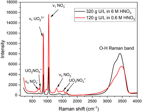
Figure 1. Raman spectrum of two U (VI) solutions in 0.6 or 6 M HNO₃, with several primary peaks labeled.

In addition to uranyl peaks, the primary nitrate bands occurred near 1,047 cm⁻¹ (ν₁ symmetric), 1,350 cm⁻¹ (ν₃ asymmetric), and 716 cm⁻¹ (ν₄ in-plane deformation). The Raman O–H band is composed of multiple peaks from approximately 3,100 to 3,700 cm⁻¹ corresponding to water molecules in unique local environments. Several species of U (VI), NO₃⁻, and HNO₃ affect the profile of the O–H band. The band can be used to quantify strong acid concentration and other ions at high-enough concentrations to perturb the water bonding network in solution (Casella et al., 2013).

Lower-intensity NO₃⁻, UO₂(NO₃)⁺, and HNO₃ peaks can become more intense or change shape upon increasing U(VI) and HNO₃ concentrations. For example, the NO₃⁻ ν₄ in-plane deformation peak splits into two bands when interacting with cations at higher concentrations. Additionally, the dissociation of HNO₃ to H⁺ and NO₃⁻ above 1 M HNO₃ is not complete; HNO₃ can be identified at higher acid concentrations above approximately 3 M by the peak near 968 cm⁻¹ (Ziouane and Leturcq, 2018). The most resolved UO₂(NO₃)⁺ peak occurred near 750 cm⁻¹, but additional peaks occurred near 1,542 and 1,620 cm⁻¹. The range of HNO₃ concentrations resulted in the formation of several species, most of which were spectrally active, including UO₂²⁺, UO₂(NO₃)⁺, UO₂(NO₃)₂, NO₃⁻, H⁺, and HNO₃, several of which have concentration-dependent features in solution. However, with exception to the uranyl symmetric stretching mode, most features observed in the Raman spectra are confounding and covarying and are therefore best modeled using multivariate analysis.

3.2 D-optimal design

Supervised chemometric regression models depend on the selection of a training set. Training set selection is often up to the user to decide, or a full factorial design can be used. User selection creates the potential for significant user bias and full factorial designs produce unnecessarily large sample sets (Czitrom, 1999). This work evaluates whether a D-optimal design–selected Y concentration matrix can result in robust PLSR and SVR models and determines the minimum number of samples and the type needed to build robust chemometric models. In other words, this study determines if the variance captured in Y by the D-optimal design captures the necessary X-variance in the spectral matrix. Developing a generalized D-optimal sample selection approach that applies to numerous spectroscopy systems will make the method practical for widespread use and more efficient for model development and implementation. Although various optical techniques with chemometric methods have been evaluated for monitoring U(VI) and HNO₃, none have attempted to generalize the training set while minimizing the sample size using this type of experiment design criterion (Felmy et al., 2023).

The D-optimal design approach allows a researcher to select sample concentrations within a consistent statistical framework and with minimal user bias. A D-optimal design was used to select U (VI) and HNO₃ concentrations (Supplementary Table S3). The concentration range of the design was chosen such that the scale went from 1 to 10 for each analyte. After generating the design, the concentration range was scaled to cover the entire range of concentrations [10–300 g L⁻¹U(VI)] or match the acid level range (0.6–6 M HNO₃). In the case of analyte concentration ranges that span more than one order of magnitude, the scaling approach creates a more balanced set of concentrations over an extended range and a model that can readily adapt to various analytes. The designed approach can readily scale to at least 10 continuous variables and additional discrete variables to account for numerous species and perturbations that would be encountered in some complex process conditions (Sadergaski et al., 2024).

The fraction of design space can be used to determine whether a design will capture the anticipated variation in a data set (Zahran et al., 2003). Based on previous work, a fraction of design space (FDS) near 0.98 was achieved using the six required model points, and an additional five LOF points, which suggests that 11 samples would be sufficient to train a robust PLSR model (Sadergaski et al., 2022b). This metric is consistent between statistically equivalent computer-generated designs, even when slightly different concentration values are selected. However, the design does not consider X spectra, so the relationship of the concentration matrix (Y) to the resulting PLSR model is empirically derived. Previous works have shown that this FDS coverage is sufficient to build robust PLS2 and PLS1 models but were mostly applied to simpler spectroscopy datasets (Bondi et al., 2012; Sadergaski et al., 2020; Sadergaski and Andrews, 2022; Sadergaski et al., 2023; Sadergaski et al., 2024). To understand how universal this metric is, the design must be generalized and tested on more complex systems, preferably with some multicollinear effects, to see if the metric holds.

3.3 PLS2 model optimization

PLS2 models were used to correlate spectral features to analyte concentration values using three Y variables [U(VI) (g L⁻¹), HNO₃ (M), and total nitrate (M)]. Multivariate analysis provides several benefits compared to univariate options including the ability to account for changing band properties (i.e., position, width, shape), multivariate signal averaging, and diagnostic capabilities (e.g., outlier detection) of an over-determined system (Pelletier, 2003). Nitrate concentration was treated as its own Y variable because the total nitrate concentration depended on both the UO₂(NO₃)₂ and HNO₃ added to the system. The entire D-optimal set of 16 calibration samples was used to build PLS2 models, and the prediction performance was tested on a separate set of 27 samples (validation set). Four latent variables were included in each PLS2 model. This inclusion was based on the last significant decrease in RMSECV (Figure 2). The last reasonable increase in explained Y-variance also occurred at this point, although it is difficult to see this visually in Figure 2. With four latent variables, 99.85% of the total Y-variation in the dataset was captured by the calibration and 99.68% by CV. Similar calibration and validation RMSEs and explained Y-variance values in Figure 2 suggest that the model is balanced with 4 LVs. Evaluation of the X-loadings and regression coefficient plots revealed that the uranyl and nitrate symmetric stretching peaks likely contribute most to the structured variation in the dataset, but other peaks in the spectrum are also important in the regression, including the water band and lower-intensity peaks (Supplementary Figure S2).

Figure 2

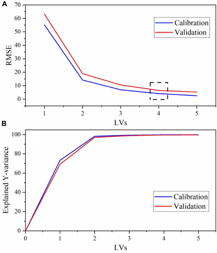
Figure 2. PLS2 model with preprocessing (A) RMSE and (B) explained Y-variance vs. the number of LVs. The dashed box corresponds to the optimal number of LVs.

In this first comparison, a PLS2 model without preprocessing and one with a baseline offset, SNV, and mean centering were compared (Table 1). Additional preprocessing combinations were evaluated (Sadergaski et al., 2022b) but did not make substantial improvements in lowering the percent RMSEP. Prediction values of percent RMSEP less than 10% are considered satisfactory, but less than 5% is considered strong (Andrews and Sadergaski, 2023). RMSEC measures the dispersion of calibration samples about the regression line. The standard error (SE) is corrected for bias, and similar values of RMSEP and SEP indicate that bias is insignificant (Faber, 1999). Bias measures whether points lie systematically above or below the regression line, and values close to zero indicate a random distribution.

Table 1

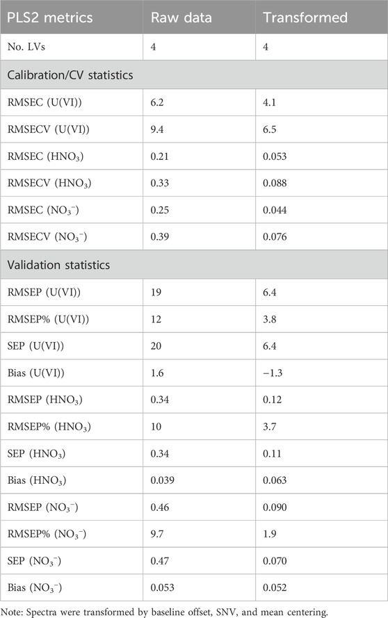
Table 1. PLS2 model calibration (C), cross calibration (CV), and prediction (P) statistics for each analyte with preprocessing and no preprocessing.

Calibration, CV, and prediction statistics were used to evaluate if preprocessing improved the PLS2 models (Table 1). The entire spectrum was modeled to see how well the models could cope with each feature. Trimming spectra regions to include the most dominant peaks was tested but did not substantially change the results. RMSEC, RMSECV, and RMSEP values for U(VI) (g L⁻¹), HNO₃ (M), and NO₃⁻ (M) were similar, which suggests that the model was balanced and able to predict new samples well. Each analyte for the PLS2 model in Table 1 had slope and R² values of the calibration plot greater than 0.99. RMSE and standard error (SE) values for the calibration, CV, and prediction were similar for all models in Table 1, indicating that each model had minimal bias.

Percent RMSEP values for each analyte predicted by the PLS2 model built with preprocessing was below the 5% target. On the contrary, the percent RMSEP values for the PLS2 model built with no preprocessing (i.e., raw data) achieved near 10% or greater. This result emphasizes how much preprocessing can improve model performance and make it more resilient to artifacts in the X matrix that are not correlated to the Y matrix (Sadergaski et al., 2022b). The limit of detection values for U(VI) based on a simple univariate check suggested that limits of detection were near 0.5 g L⁻¹ U(VI) (Supplementary Figures S3, S4). However, with respect to modeling the entire system, the RMSEP values provide an estimate of the ± deviation in the predictions. This result suggests that the PLS2 model limit of detection for U(VI) was near approximately 6 g L⁻¹ U(VI). The validation set contained samples at concentrations within and slightly below and above the calibration set. Each PLS2 preprocessed model prediction fell within the Hotelling’s T² critical limit (p-value 5%), indicating that each sample fell within the multivariate space described by the model (Supplementary Figure S5).

3.4 Comparing PLS1 with SVR

PLS1 and SVR models were evaluated based on U(VI) and HNO₃ concentration determination accuracy because these were the primary analytes of interest. SVR models in Vektor Direktor v2.0 could only be built for one Y variable, so the SVR results were only compared to PLS1 models. PLS1 and SVR models were built for U(VI) (g L⁻¹) and HNO₃ (M) to evaluate the performance of linear PLSR and nonlinear SVR models. Techniques such as principal component regression, locally weighted regression, and PLSR have been applied to similar datasets, although SVR could provide benefits compared with the former linear options (Burck, 1992; Kirsanov et al., 2017; Felmy et al., 2023). Two types of SVMs were tested: Type 1 (C-SVM) and Type 2 (ν-SVM). Type 1 performed better, having somewhat-balanced RMSE and RMSECV values and lower RMSEP values.

The PLSR and SVR model results are presented in Table 2. The performance of PLS1 models was similar to the PLS2 model (compare Table 1). The PLS1 model percent RMSEP values for U(VI) and HNO₃ were 3.8% and 3.7%, respectively, indicating nearly identical strong performance. This result was unexpected because PLS1 models for U(VI) were expected to have lower percent RMSEP values owing to the nearly linear response of the uranyl symmetric stretching mode, and PLS1 models for HNO₃ described the more multivariate response of HNO₃ spectral features. This could be a result of nonlinearity in lower-intensity UO₂ (NO₃)⁺ peaks, but trimming the spectra to only include the uranyl symmetric stretching mode did not make significant improvements in RMSEP (data not shown here). Even though PLSR is a linear model, it can describe some nonlinearity in spectral systems using combinations of LVs. The RMSEC, RMSECV, and RMSEP values were balanced for U(VI) and HNO₃, indicating robust and stable regression models.

Table 2

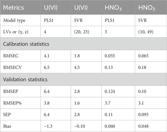
Table 2. Values for PLS1 and SVR models using the entire 16 sample training set.

The two SVR hyperparameters (γ and ε) were optimized by minimizing the difference between RMSEV and RMSECV. The γ value describes the distance the influence of a single training sample reaches from the separation line. SVR tends to overfit when γ is large and underfit when γ is small. The ε value, referred to as the epsilon intensive loss function, seeks to optimize the regression bounds. In each SVR model, moderate ε and γ values near the center of the heat maps were chosen to mitigate overfitting and underfitting (see Supplementary Figure S6).

SVR models for U(VI) and HNO₃ performed better than the PLS1 models in terms of percent RMSEP, SEP, and bias. The top SVR models for U(VI) and HNO₃ resulted in percent RMSEP values of 1.6% and 3.1%, respectively. The percent RMSEP value for U(VI) approached the error in the sample preparation (see detailed discussion in the Supplementary Material), suggesting that the model accounted for nearly all the spectral variation. RMSEP and SEP values were similar for all models in Table 2, indicating that each model had minimal bias despite comprising only 16 samples. SVR model ε and γ values and the number of PLS1 model LVs are shown in Table 2.

It is useful to show where the predicted values fall in comparison with the target line (1:1) by evaluating parity plots of model predictions vs. reference values. Parity plots of the predicted U(VI) and HNO₃ concentrations relative to the reference values are shown in Figure 3. The calibration and prediction values fall close to the 1:1 line, indicating strong performance. The highest-concentration U(VI) sample in the validation set was slightly higher than the highest concentration in the calibration set. The PLS1 model underpredicted this sample (Figure 3A), while the SVR model predicted it much closer to the 1:1 line (Figure 3C)

Figure 3

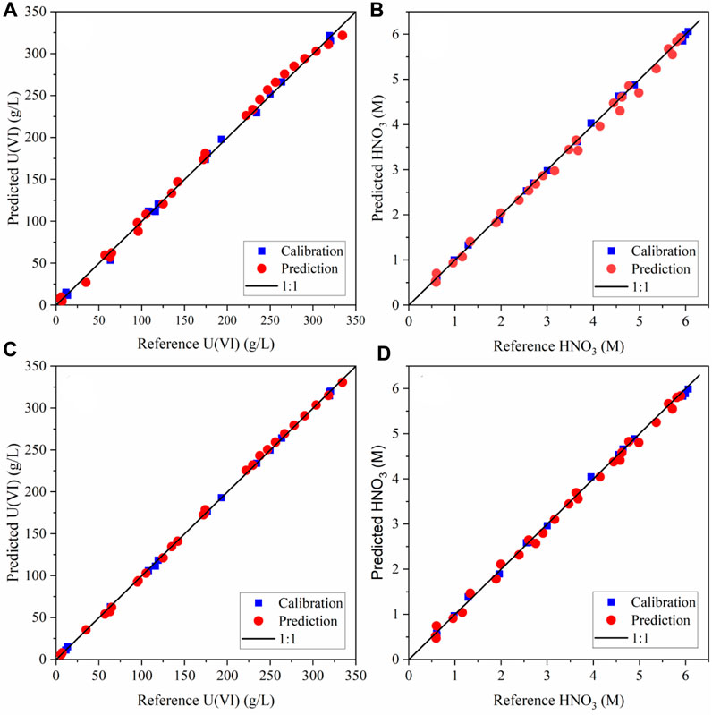
Figure 3. Parity plot pf the calibration and prediction data for (A) PLS1 U (VI) model, (B) PLS1 HNO₃ model, (C) SVR U (VI) model, and (D) SVR HNO₃ model.

3.5 Comparing LOF points

There are numerous examples of minimizing training sets for PLSR regression but very few for SVR models (Bondi et al., 2012; Sadergaski et al., 2022b). It is important to empirically determine the relationship between sample set size and SVR model performance (Rodriguez-Perez et al., 2017). It is not apparent whether nonlinear SVR models must be trained with a different number of calibration standards then PLSR. Testing will determine if the D-optimal sample selection approach, mostly evaluated for PLSR model development, is also amenable to minimizing samples in training sets for SVR (Rodriguez-Perez et al., 2017; Sadergaski et al., 2022b). When many samples are regressed and a model is too complex, variance dominates the uncertainty. If the model comprises too few sampling points, then bias dominants the uncertainty (i.e., bias–variance trade-off) (Faber, 1999). An ideal model would balance variance and bias and use the minimum number of samples needed to achieve the measurement accuracy required.

A relatively wide range of ε and γ values resulted in robust SVR predictive models. Similar regions of the heat map for γ and ε values were chosen for SVR LOF point comparisons. The SVR prediction performance was somewhat similar despite using various ε and γ values, but the variables did require some fine-tuning for optimization. Further optimization could be pursued in future work. The suggested range of values in the heat map often presented the lowest RMSECV values but also unreasonably low RMSEC values for U (e.g., 0.1 for U). Thus, various regions were evaluated to balance RMSEC and RMSECV by finding a point of RMSEC near 1 or greater for U. Any lower RMSEC values are considered unrealistic compared with the error in sample preparation. For example, when using just the required model points, a wide range of ε and γ values (e.g., 14.3, 30.6) generated a RMSEC of 0.1 and RMSECV of 20.43, which resulted in an RMSEP of 8.2. Finding a slightly different combination (13.4, 22.3) with a somewhat more reasonable RMSEC of 1.3 and similar RMSECV of 20.8 resulted in an RMSEP value of 9.3. In either case, averaging RMSEC and RMSECV resulted in a realistic estimate of RMSEP.

CV statistics that are high when compared with prediction metrics may imply that a model is not balanced. It could also mean that no redundant samples are in the calibration set, so that when one is left out, it has a major effect on the performance, inflating the CV metrics. RMSECV provides an estimate of the RMSEP, but each RMSECV statistic for PLS1 and SVR U models built using just six samples in the calibration set greatly overestimated RMSEP (Figure 4). Thus, when minimizing samples in the calibration set, it is more important that the calibration and prediction metrics are comparable.

Figure 4

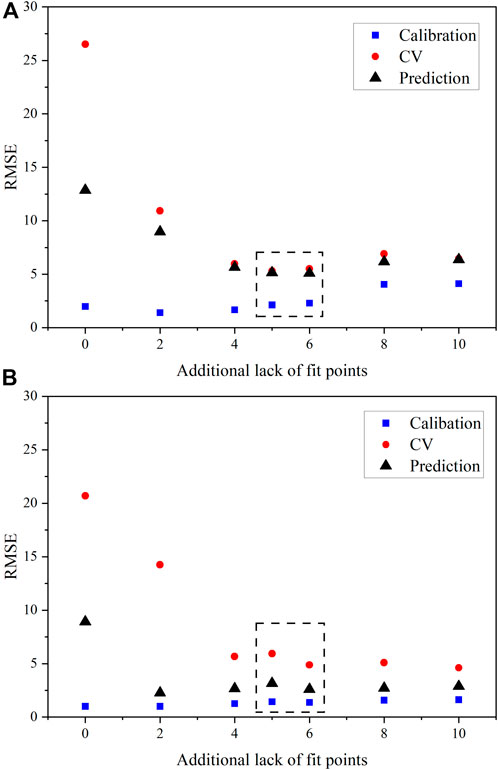
Figure 4. RMSE values for U(VI) with varying LOF points included in the calibration set for (A) PLS1 models and (B) SVR models. The dashed black box correspondes the optimal number of samples suggested by FDS considerations.

RMSEC, RMSECV, and RMSEP values for PLS1 and SVR models built for U (VI) are shown in Figure 4. The region corresponding to 11 and 12 total samples is marked by a dashed rectangle. Per FDS, 11 calibration samples were expected to provide the minimum number of samples needed for sufficient sample coverage while balancing RMSE values and maintaining bias. The percent RMSEP values for PLS1 U(VI) models with just 11 samples outperformed models built with 14 and 16 D-optimal samples, approaching percent RMSEP values close to 3% as opposed to nearly 4% (Figure 4A) This emphasizes the significance of sample set size and composition. The RMSECV also provided a reasonable estimate of the RMSEP values. The bias for PLS1 U (VI) models remained essentially constant when 10 or greater samples were included in the calibration set, which indicates that enough samples were used to train the models. Thus, the presumed optimal sample set of 11 per the 0.98 FDS metric held true. However, 12 samples would also be a reasonable estimate of samples as the first quantity resulting in an FDS (1.0).

RMSE values were less balanced for SVR U(VI) models (Figure 4B). The RMSECV decreased with increasing LOF points, as expected. Interestingly, the sample set comprising just eight samples (two LOF points) resulted in the lowest percent RMSEP value of 1.3%. The bias of predictions also remained consistent and near zero when eight or more samples were used in the regression. The nature of the linear uranyl symmetric stretching mode response likely resulted in somewhat unbalanced RMSEC and RMSEP values for SVR U(VI) models. To achieve a better balance between RMSEC, RMSECV, and RMSEP values, more samples (8 or 10 LOF points) were required in the model. The difference between RMSEC and RMSEP values for the 10-sample training set was reasonable, and if sample size is important and the fitting aspect is less important than a model’s predictive ability, the 11-sample set would be acceptable.

The behavior of model performance with varying LOF points for HNO₃ was unique compared with U(VI). The concentration range of HNO₃ was smaller than U(VI), which could explain why fewer samples were needed in the calibration set. The SVR HNO₃ model with no LOF points (i.e., six samples) had the largest gap between RMSEC, RMSECV, and RMSEP (Figure 5A). The six samples fit very well in the calibration model, and leaving one out CV had a major effect on RMSECV. However, the RMSEP values for models built with varying LOF points remained approximately constant. Finding balanced ε and γ values in the heat map for SVR models and HNO₃ was simpler than U(VI). The RMSEC and RMSECV values were more balanced throughout the heat map plot in the blue regions. It also appeared that fewer samples were required because the RMSEC and RMSEP values were balanced even with six samples (required model points). This result was somewhat unexpected given the covarying spectral response of HNO₃ compared with the more linear response of the uranyl symmetric mode.

Figure 5

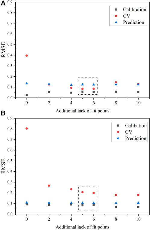
Figure 5. RMSE values for HNO₃ with varying LOF points included in the calibration set for (A) PLS1 models and (B) SVR models. The dashed black box correspondes the optimal number of samples suggested by FDS considerations.

The difference in RMSEC and RMSEP was more than a factor of two for SVR models in Figure 5. However, this result is expected to some degree given the prediction performance on the larger validation set (27 samples) compared with the smaller calibration set (6–16 samples). Ultimately, it appears that having a minimum of eight samples resulted in relatively robust predictive PLS1 and SVR models for HNO₃, and SVR models provided lower RMSEP values for HNO₃ (0.10). This result suggests that the designed calibration set provides a statistically sound method for selecting samples for both modeling types. Thus, the designed approach applies to SVR modeling for models describing both U(VI) and HNO₃. The D-optimal selection approach for calibration sets applies to both PLSR and SVR models.

The 11-sample training set that balances prediction performance and resources is highlighted in Supplementary Table S3. The 11-sample training shown in Supplementary Table S3 could be leveraged in future studies as the foundational samples needed to account for U(VI) and HNO₃. Additional samples will be added when accounting for additional variables. This set of 5 LOF points was chosen at random out of the available 10 LOF samples. Differing combinations of 5 LOF points randomly selected out of the 10 possible points resulted in similar performance (data not shown here). Researchers have shown that performance changes depending on which LOF points are included (Andrews and Sadergaski, 2023). It is recommended to analyze additional samples with disparate datasets; generating a D-optimal model with just 5 LOF points, as opposed to the 10 evaluated in this study, may yield slightly different results because varying combinations of LOF points can yield different prediction performance.

Understanding the performance of PLSR and SVR models with minimized sample sets has great benefits for numerous applications. It also provides a starting point for future studies that will aim to include varying temperature and fission/corrosion product levels, where the number of training set samples will increased substantially. The designed approach in this work can be extended to include additional factors that could be encountered in real-world systems (Sadergaski et al., 2024). Complex spectra features need to be accounted for in applications like nuclear fuel reprocessing where self-absorption effects, temperature fluctuations, and other things will be prevalent (Moulin et al., 1996). In this situation, we hypothesize that a non-linear SVR model may be advantageous compared to more traditional methods (e.g., PLSR).

Prior to this work, it was unclear how sample set size and composition for SVR and PLSR models would compare and whether a D-optimal designed approach could be leveraged for SVR model training set selection. If SVR required more samples than PLSR, then the designed approach and integration of such a technique for process monitoring would be more challenging. The results presented herein are promising and suggest that continued work to evaluate SVR for monitoring complex chemical processes in the nuclear field and beyond is warranted.

4 Conclusion

Results of this study indicate that D-optimal design–selected training sets are useful for optimizing PLSR and SVR regression models that may be used for quantitative measurements of U(VI) and HNO₃ by Raman spectroscopy over a wide range of concentrations relevant to nuclear fuel cycle processes. A D-optimal design can effectively minimize time and materials associated with training chemometric models while maintaining or even improving prediction performance. Nonlinear SVR models outperformed more-traditional linear PLSR models with lower percent RMSEP values for both U(VI) (1.5%) and HNO₃ (3.1%). Even with the nearly linear response of the uranyl symmetric stretching mode, SVR model optimization required more adjustments of ε and γ values to tune the performance than attempts to model the covarying spectral response of HNO₃. Considering calibration and CV statistics alone may yield over- and underestimated estimates of prediction performance, when evaluating designed training sets, it is essential to test the model’s prediction performance on validation samples not included in the calibration set. Future work will leverage the training set and modeling capabilities developed in this work for the analysis of more complex systems with additional factors (e.g., metal cation nitrate and dynamic temperature). Findings presented here provide promising results for efficient and effective chemometric applications within and beyond the nuclear field.

Data availability statement

The original contributions presented in the study are included in the article/Supplementary Material, further inquiries can be directed to the corresponding authors.

Author contributions

LS: Conceptualization, Formal Analysis, Methodology, Writing–original draft. JE: Data curation, Validation, Writing–review and editing. LD: Funding acquisition, Supervision, Writing–review and editing. JB: Funding acquisition, Project administration, Supervision, Writing–review and editing.

Funding

The author(s) declare that financial support was received for the research, authorship, and/or publication of this article. For this work was provided by the Advanced Research Projects Agency-Energy under contract DE-AC05-00OR22725, which supported L.R.S., J.D.E, and L.H.D, and under Award Number DE-AR0001689, which supported J.D.B. The information, data, or work presented herein was funded in part by the Advanced Research Projects Agency-Energy (ARPA-E), U.S. Department of Energy, under contract DE-AC05-00OR22725 and Award Number DE-AR0001689.

Acknowledgments

This work used resources at the Radiochemical Engineering Development Center operated by the US Department of Energy’s Oak Ridge National Laboratory.

Rights and Permissions

This submitted manuscript has been authored by UT-Battelle, LLC, under contract DE-AC05-00OR22725 in collaboration with the University of Alabama at Birmingham under Award Number DE-AR0001689 with the U.S. Department of Energy. The United States Government retains and the publisher, by accepting the article for publication, acknowledges that the United States Government retains a non-exclusive, paid-up, irrevocable, world-wide license to publish or reproduce the published form of this manuscript, or allow others to do so, for the United States Government purposes. The Department of Energy will provide public access to these results of federally sponsored research in accordance with the DOE Public Access Plan (http://energy.gov/downloads/doe-public-access-plan).

Conflict of interest

The authors declare that the research was conducted in the absence of any commercial or financial relationships that could be construed as a potential conflict of interest.

Publisher’s note

All claims expressed in this article are solely those of the authors and do not necessarily represent those of their affiliated organizations, or those of the publisher, the editors and the reviewers. Any product that may be evaluated in this article, or claim that may be made by its manufacturer, is not guaranteed or endorsed by the publisher.

Author disclaimer

This manuscript was prepared as an account of work sponsored by an agency of the United States Government. Neither the United States Government nor any agency thereof, nor any of their employees, makes any warranty, express or implied, or assumes any legal liability or responsibility for the accuracy, completeness, or usefulness of any information, apparatus, product, or process disclosed, or represents that its use would not infringe privately owned rights. Reference herein to any specific commercial product, process, or service by trade name, trademark, manufacturer, or otherwise does not necessarily constitute or imply its endorsement, recommendation, or favoring by the United States Government or any agency thereof. The views and opinions of authors expressed herein do not necessarily state or reflect those of the United States Government or any agency thereof.

Supplementary material

The Supplementary Material for this article can be found online at: https://www.frontiersin.org/articles/10.3389/fnuen.2024.1411840/full#supplementary-material

References

Andrews, H. B., and Sadergaski, L. R. (2023). Leveraging visible and near-infrared spectroelectrochemistry to calibrate a robust model for Vanadium(IV/V) in varying nitric acid and temperature levels. Talanta 259, 124554. doi:10.1016/j.talanta.2023.124554

PubMed Abstract | CrossRef Full Text | Google Scholar

Bondi, Jr. R. W., Igne, B., Drennen III, J. K., and Anderson, C. A. (2012). Effect of experimental design on the prediction performance of calibration models based on near-infrared spectroscopy for pharmaceutical applications. Appl. Spectrosc. 66 (12), 1442–1453. doi:10.1366/12-06689

PubMed Abstract | CrossRef Full Text | Google Scholar

Bryan, S. A., Levitskaia, T. G., Johnsen, A. M., Orton, C. R., and Peterson, J. M. (2011). Spectroscopic monitoring of spent nuclear reprocessing streams: an evaluation of spent fuel solutions via Raman, visible, and near-infrared spectroscopy. Radiochim. Acta 99, 563–571. doi:10.1524/ract.2011.1865

CrossRef Full Text | Google Scholar

Burck, J. (1992). Spectrophotometric determination of uranium and nitric acid by applying partial least-squares regression to uranium(VI) absorption spectra. Anal. Chim. Acta 254, 159–165. doi:10.1016/0003-2670(91)90022-w

CrossRef Full Text | Google Scholar

Burns, J. D., and Moyer, B. A. (2016). Group hexavalent actinide separations: a new approach to used nuclear fuel recycling. Inorg. Chem. 55, 8913–8919. doi:10.1021/acs.inorgchem.6b01430

PubMed Abstract | CrossRef Full Text | Google Scholar

Casella, A. J., Levitskaia, T. G., Peterson, J. M., and Bryan, S. A. (2013). Water O–H stretching Raman signature for strong acid monitoring via multivariate analysis. Anal. Chem. 85, 4120–4128. doi:10.1021/ac4001628

PubMed Abstract | CrossRef Full Text | Google Scholar

Chen, T., and Guestrin, C. (2016). “XGBoost: a scalable tree boosting system,” in Proceedings of the 22nd SIGKDD Conference on Knowledge Discovery and Data Mining, San Francisco, California, USA, 785–794.

Google Scholar

Colle, J.-Y. C., Manara, D., Geisler, T., and Konings, R. J. M. (2020). Advances in the application of Raman spectroscopy in the nuclear field. Spectrosc. Eur. 32, 9–13.

Google Scholar

Couston, L., Pouyat, D., Moulin, C., and Decambox, P. (1995). Speciation of uranyl species in nitric acid medium by time-resolved laser-induced fluorescence. Appl. Spectrosc. 49, 349–353. doi:10.1366/0003702953963553

CrossRef Full Text | Google Scholar

Czitrom, V. (1999). One-factor-at-a-time versus designed experiments. Am. Stat. 53 (2), 126–131. doi:10.2307/2685731

CrossRef Full Text | Google Scholar

Deiss, L., Margenot, A. J., Culman, S. W., and Demyan, M. S. (2020). Tuning support vector machines regression models improves prediction accuracy of soil properties in MIR spectroscopy. Geoderma 365, 114227. doi:10.1016/j.geoderma.2020.114227

CrossRef Full Text | Google Scholar

Einkauf, J. D., and Burns, J. D. (2020). Solid state characterization of oxidized actinides co-crystallized with uranyl nitrate hexahydrate. Dalton Trans. 49, 608–612. doi:10.1039/c9dt04000e

PubMed Abstract | CrossRef Full Text | Google Scholar

Faber, N. M. (1999). A closer look at the bias-variance trade-off in multivariate calibration. J. Chemom. 13, 185–192. doi:10.1002/(sici)1099-128x(199903/04)13:2<185::aid-cem538>3.3.co;2-e

CrossRef Full Text | Google Scholar

Felmy, H. M., Bessen, N. P., Lackey, H. E., Bryan, S. A., and Lines, A. M. (2023). Quantification of uranium in complex acid media: understanding speciation and mitigating for band shifts. ACS Omega 8, 41696–41707. doi:10.1021/acsomega.3c06007

PubMed Abstract | CrossRef Full Text | Google Scholar

Guillaume, B., Begun, G. M., and Hahn, R. L. (1982). Raman spectrometric studies of cation cation complexes of pentavalent actinides in aqueous perchlorate solutions. Inorg. Chem. 21, 1159–1166. doi:10.1021/ic00133a055

CrossRef Full Text | Google Scholar

Guo, S., Popp, J., and Bocklitz, T. (2021). Chemometric analysis in Raman spectroscopy from experimental design to machine learning–based modeling. Nat. Protoc. 16, 5426–5459. doi:10.1038/s41596-021-00620-3

PubMed Abstract | CrossRef Full Text | Google Scholar

Ikeda-Ohno, A., Hennig, C., Tsushima, S. Z., Scheinost, A. C., Bernhard, G., and Yaita, T. (2009). Speciation and structural study of U(IV) and -(VI) in perchloric and nitric acid solutions. Inorg. Chem. 48, 7201–7210. doi:10.1021/ic9004467

PubMed Abstract | CrossRef Full Text | Google Scholar

Kirsanov, D., Rudnitskaya, A., Legin, A., and Babain, V. (2017). UV-VIS spectroscopy with chemometric data treatment: an option for on-line control in nuclear industry. J. Radioanal. Nucl. Chem. 312, 461–470. doi:10.1007/s10967-017-5252-8

CrossRef Full Text | Google Scholar

Lascola, R., O’Rourke, P. E., and Kyser, E. A. (2017). A piecewise local partial least squares (PLS) method for the quantitative analysis of plutonium nitrate solutions. Appl. Spectrosc. 71, 2579–2594. doi:10.1177/0003702817734000

PubMed Abstract | CrossRef Full Text | Google Scholar

Lines, A. M., Hall, G. G., Asmussen, S., Allred, J., Sinkov, S., Heller, F., et al. (2020). Sensor fusion: comprehensive real-time, on-line monitoring for process control via visible, near-infrared, and Raman spectroscopy. ACS Sens. 5, 2467–2475. doi:10.1021/acssensors.0c00659

PubMed Abstract | CrossRef Full Text | Google Scholar

Matusi, T., Fujimori, H., and Suzuki, K. (1988). Effects of coexisting ions upon UO₂²⁺ fluorescence in fuel reprocessing solutions. J. Nucl. Sci. Technol. 25, 868–874. doi:10.3327/jnst.25.868

CrossRef Full Text | Google Scholar

Moulin, C., Decambox, P., Couston, L., and Pouyat, D. (1994). Time-resolved laser-induced fluorescence of UO₂²⁺ in nitric acid solutions: comparison between nitrogen and tripled Nd-YAG laser. J. Nucl. Sci. Technol. 31, 691–699. doi:10.3327/jnst.31.691

CrossRef Full Text | Google Scholar

Moulin, C., Decambox, P., Mauchien, P., Pouyat, D., and Couston, L. (1996). Direct uranium(VI) and nitrate determinations in nuclear reprocessing by time-resolved laser-induced fluorescence. Anal. Chem. 68, 3204–3209. doi:10.1021/ac9602579

CrossRef Full Text | Google Scholar

Pelletier, M. J. (2003). Quantitative analysis using Raman spectrometry. Appl. Spectrosc. 57, 20–42. doi:10.1366/000370203321165133

PubMed Abstract | CrossRef Full Text | Google Scholar

Rodriguez-Perez, R., and Bajorath, J. (2022). Evolution of support vector machine and regression modeling in chemoinformatics and drug discovery. J. Comput. Aided. Mol. Des. 36, 355–362. doi:10.1007/s10822-022-00442-9

PubMed Abstract | CrossRef Full Text | Google Scholar

Rodriguez-Perez, R., Vogt, M., and Bajorath, J. (2017). Influence of varying training set composition and size on support vector machine-based prediction of active compounds. J. Chem. Inf. Model. 57, 710–716. doi:10.1021/acs.jcim.7b00088

PubMed Abstract | CrossRef Full Text | Google Scholar

Sadergaski, L. R., and Andrews, H. B. (2022). Simultaneous quantification of uranium(VI), samarium, nitric acid, and temperature with combined ensemble learning, laser fluorescence, and Raman scattering for real-time monitoring. Analyst 147, 4014–4025. doi:10.1039/d2an00998f

PubMed Abstract | CrossRef Full Text | Google Scholar

Sadergaski, L. R., Andrews, H. B., and Wilson, B. A. (2024). Comparing sensor fusion and multimodal chemometric models for monitoring U(VI) in complex environments representative of irradiated nuclear fuel. Anal. Chem. 96, 1759–1766. doi:10.1021/acs.analchem.3c04911

PubMed Abstract | CrossRef Full Text | Google Scholar

Sadergaski, L. R., DePaoli, D. W., and Myhre, K. G. (2020). Monitoring the caustic dissolution of aluminum alloy in a radiochemical hot cell using Raman spectroscopy. Appl. Spectrosc. 74, 1252–1262. doi:10.1177/0003702820933616

PubMed Abstract | CrossRef Full Text | Google Scholar

Sadergaski, L. R., Hagar, T. J., and Andrews, H. B. (2022b). Design of experiments, chemometrics, and Raman spectroscopy for the quantification of hydroxylammonium, nitrate, and nitric acid. ACS Omega 7, 7287–7296. doi:10.1021/acsomega.1c07111

PubMed Abstract | CrossRef Full Text | Google Scholar

Sadergaski, L. R., Manard, B. T., and Andrews, H. B. (2023). Analysis of trace elements in uranium by inductively coupled plasma-optical emission spectroscopy, design of experiments, and partial least squares regression. J. Anal. At. Spectrom. 38, 800–809. doi:10.1039/d3ja00013c

CrossRef Full Text | Google Scholar

Sadergaski, L. R., Myhre, K. G., and Delmau, L. H. (2022a). Multivariate chemometric methods and Vis-NIR spectrophotometry for monitoring plutonium-238 anion exchange column effluent in a radiochemical hot cell. Talanta Open 5, 100120. doi:10.1016/j.talo.2022.100120

CrossRef Full Text | Google Scholar

Steinbach, D. S., Anderson, C. A., McGeorge, G., Igne, B., Bondi, R. W., and Drennen, J. K. (2017). Calibration transfer of a quantitative transmission Raman PLS model: direct transfer vs. Global modeling. J. Pharm. Innov. 12, 347–356. doi:10.1007/s12247-017-9299-4

CrossRef Full Text | Google Scholar

Wold, S., Josefson, M., Gottfries, J., and Linusson, A. (2003). The utility of multivariate design in PLS modeling. J. Chemom. 18, 156–165. doi:10.1002/cem.861

CrossRef Full Text | Google Scholar

Wold, S., and Sjostrom, M. (1998). Chemometrics, present and future success. Chemom. Intel. Lab. Syst. 44, 3–14. doi:10.1016/s0169-7439(98)00075-6

CrossRef Full Text | Google Scholar

Wold, S., Sjostrom, M., and Eriksson, L. (2001). PLS-regression: a basic tool of chemometrics. Chemom. Intell. Lab. Syst. 58, 109–130. doi:10.1016/s0169-7439(01)00155-1

CrossRef Full Text | Google Scholar

Zahran, A. R., Anderson-Cook, C. M., and Myers, R. H. (2003). Fraction of design space to assess prediction capability of response surface designs. J. Qual. Tech. 35, 377–386. doi:10.1080/00224065.2003.11980235

CrossRef Full Text | Google Scholar

Ziouane, Y., and Leturcq, G. (2018). New modeling of nitric acid dissociation function of acidity and temperature. ACS Omega. 3, 6566–6576. doi:10.1021/acsomega.8b00302

PubMed Abstract | CrossRef Full Text | Google Scholar