 Chengyuan Li
 Meifu Li1*
 Zhifang Qiu
95% of researchers rate our articles as excellent or good
Learn more about the work of our research integrity team to safeguard the quality of each article we publish.
Find out more
ORIGINAL RESEARCH article
Front. Nucl. Eng. , 07 February 2024
Sec. Nuclear Reactor Design
Volume 3 - 2024 | https://doi.org/10.3389/fnuen.2024.1339457
This article is part of the Research Topic Artificial Intelligence in Advanced Nuclear Reactor Design View all 6 articles
Introduction: The accurate prognosis of reactor accidents is essential for deploying effective strategies that prevent radioactive releases. However, research in the nuclear sector is limited. This paper introduces a novel Temporal Fusion Transformer (TFT) model-based method for accident prognosis that incorporates multi-headed self-attention and gating mechanisms.
Methods: Our proposed method combines multi-headed self-attention and gating mechanisms of TFT with multiple covariates to enhance prediction accuracy. Additionally, we employ quantile regression for uncertainty assessment. We apply this method to the HPR1000 reactor to predict outcomes following loss of coolant accidents (LOCAs).
Results: The experimental results reveal that our proposed method outperforms existing deep learning-based prediction models in both prediction accuracy and confidence intervals. We also demonstrate increased robustness through interference experiments with varying signal-to-noise ratios and ablation studies on static covariates.
Discussion: Our method contributes to the development of intelligent and reduced-staff maintenance methods for reactor systems, showcasing its ability to effectively extract and utilize features of static and historical covariates for improved predictive performance.
Promoting Gen III nuclear power plants is essential to combat climate change and reduce emissions. Nuclear energy, with its low-carbon profile, is a significant contributor to global low-carbon electricity supply and overall electricity generation. This focus is critical for achieving the goal of limiting global temperature rise to 2°C by 2050 (Agency, 2021).
Currently, Gen III nuclear power technology, specifically advanced pressurized water reactors, is the dominant technology used in new nuclear power units. These reactors have the capability to minimize the frequency of core damage to less than
To mitigate the risks associated with a LOCA in nuclear reactor cores, the implementation of preemptive measures is imperative. Within the framework of HPR1000 Generation III nuclear power technology, the management of accidents is governed by a regimen of indicator-based protocols, predominantly the Optimal Recovery Protocols (ORPs) and Functional Recovery Protocols (FRPs). ORPs are reserved for clearly identifiable accidents, exemplified by substantial ruptures exceeding 34.5 cm in diameter. Conversely, FRPs are designated for scenarios that elude precise diagnosis or fall outside the definitive parameters of ORPs, such as intermediate breaches with diameters ranging from 2.5 to 34.5 cm. The precision of accident diagnosis and subsequent prognosis is paramount, enabling reactor operators to execute informed decisions to curtail the escalation of the event. The decision-making process entails a bifurcated approach: initially diagnosing the incident to yield interface data for the prognostication of reactor status, followed by forecasting the evolution of reactor conditions to facilitate strategic decisions by operators. This manuscript delineates the prognosticative process subsequent to LOCA, predicated on the diagnostic findings from the antecedent phase. Figure 1 illustrates the position of the prognostic phase within the maintenance sequence.
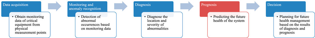
FIGURE 1. Prognosis in the sequence of reactor accident health maintenance.
A considerable number of previous explorations have been carried out in order to rapidly diagnose reactor anomalies and to foresee the process of anomalies. Most of these methods are model-based or data-based, or rule-based methods built on models and data combined with expert knowledge (Lei, 2020; Zhang et al., 2022; Zio, 2022). Currently, data-based approaches based on statistical learning and deep learning are the focus of research, due to their greater generalization ability and inference speed compared to model-based approaches, and their easier maintenance than rule-based approaches that utilize large knowledge bases.
The diagnosis of abnormal reactor operation has been explored extensively by previous works. Lin et al. (2021) developed a Nearly Autonomous Management and Control (NAMAC) framework for advanced reactors and used feedforward neural networks for the digital twin (DT) layer in the framework to quickly identify information about anomalous transients. Ayodeji et al. (2018) constructed a nuclear power plant operator operation support system based on the use of principal component analysis (PCA) and two different neural networks: an Elman-type recurrent neural network (Elman-RNN) and a radial basis neural network (RBN) for fault diagnosis. Lee et al. (2021) organized the large amount of real-time data generated by a single system and the dynamics of the individual system monitoring data by constructing two-channel 2D images and used convolutional neural networks (CNN) for feature extraction and diagnostic tasks of system anomalous transients. Wang et al. (2019) proposed a support vector machine (SVM)-based diagnosis method in order to improve the diagnostic capability of the model on a smaller number of accident instances and used an improved particle swarm optimization (PSO) method for the selection of hyperparameters of the model to achieve an improved accident classification capability in the case of small samples. Li and Lin (2021) constructed an integrated learning model using various statistical learning models and neural network models, such as SVM, random forest model (RF), k-nearest neighbor model (KNN), and fully connected neural network (FCNN), and based on multivariate voting method and weighted voting method, the model was able to achieve a rapid response and robust to noise for accident diagnosis. For more detailed information on diagnostic methods for abnormal reactor operation, please refer to the review articles (Ma and Jiang, 2011; Jiang et al., 2020; Maitloa et al., 2020; Hu et al., 2021).
Prior research has disproportionately emphasized accident diagnosis over post-accident prognosis, with a marked paucity in the prognostication of system-level parameters. Although the use of best estimation (BE) based system analysis programs, such as RELAP (Allison and Hohorst, 2010) or ARSAC (Deng et al., 2021), allows for a more accurate calculation of accidents with known parameters, their use in real-time operator manipulation is still impractical due to their slow computational speed. Consequently, the deployment of data-driven, pretrained models for accelerated inferential computations emerges as a critical alternative to enable ultra-real-time assessment of reactor status subsequent to an incident. In for the task of system state prediction after the occurrence of anomalous reactor transients, Zeng et al. (2018) used SVM to construct agent models for the thermal and physical steps of nuclear thermal coupling calculations, respectively, along with a particle filtering framework for noise filtering and prediction of system parameter measurements to achieve the system state prediction task for the Transportable Fluoride-salt-cooled High-temperature Reactor (TFHR) under reactive introduction accidents. Koo et al. (2019) used FCNN to construct a model for predicting the trend of pressure vessel (PV) water level for steam generator pipe rupture and cold/hot leg LOCA and demonstrated the superiority of this prediction method by comparing the performance of this model with a cascaded fuzzy logic neural network model (CFNN) for the same task. Zhang et al. (2020) adopted a long short-term memory network (LSTM) that is more sensitive to less data in order to improve the quantitative imbalance between the training data on the fluctuating operation category and the stable operation category, and used the model trained using this strategy for the task of predicting the reactor’s pressurizer (PRZ) water level under abnormal operation. Gurgen (2021) developed a physically constrained LSTM reactor parameter prediction method based on physical constraints in order to serve the decision layer in the NAMAC framework, and applied the method to the prediction of fuel centerline temperature in the loss-of-flow accident (LOFA) of Experimental Breeder Reactor II. However, with the exception of the few studies on reactor state prediction at the system level mentioned above, most prediction efforts have focused more on the state and remaining usable time (RUL) of subsystems or components. For example, Ramuhalli et al. (2020) used LSTM model, SVM model and nonlinear autoregressive model (NAR) to predict the operating status of feedwater and condensate system (FWCS) of boiling water reactor (BWR) for the next day and the next week, respectively. Liu et al. (2015) proposed a dynamic weight integration learning prediction method based on multiple SVM regression models, and applied the method to the leakage prediction task of the reactor first-loop coolant main pump, as well as estimated for the uncertainty of the prediction results. More RUL prognostic tasks on reactor subsystems and components are available in the review articles by Ayo-Imoru et al. (Ayo-Imoru and Cilliers, 2018) and Si et al. (Si et al., 2011).
In contrast to the nuclear sector, prognostic endeavors are becoming increasingly critical across a diverse array of industries. Predominantly, these methodologies are underpinned by extensive data analytics. Within the burgeoning domain of renewable energy, the predictive assessment of battery pack conditions post-anomalies is imperative for ensuring the operational safety of electric vehicles. Hong et al. (2019) established an accurate multi-forward-step voltage prediction method for battery systems using LSTM and validated the superiority, stability and robustness of the method using real-world data. Liu et al. (2022) proposed a joint prognostic method of AutoRegressive Integrated Moving Average model (ARIMA) and LSTM using approximate optimization method in order to improve the prediction accuracy of electric vehicle battery pack voltage. In the field of wind power generation, prediction of the degradation process of turbines and estimation of RUL is an essential means to improve the operating economics (Gao and Liu, 2021) (Saidi et al., 2017) constructed a prediction method based on spectral kurtosis and SVM regression model in order to predict the operating condition of the high-speed shaft bearing in wind turbines. Encalada-Dávila et al. (2021) constructed a method for predicting Low-speed shaft temperature under normal operation and abnormal transients using fully connected neural networks and validated the method on real-world operational data from several wind turbines. Therefore, the prognostic approach in the non-nuclear field can provide insights and inspiration for the task of prognosis of system level parameters after a reactor accident.
Deep learning has revolutionized problem-solving in various sectors through neural networks’ function approximation capabilities, using gradient descent for optimization. These networks automatically extract critical features from data. In accident process prediction, which requires temporal data modeling, recurrent neural networks (RNNs), including Elman-type, LSTM, and GRU, have been prevalent to enhance prediction accuracy. However, RNNs face challenges with long-range dependencies and uncertainty estimation in long sequences. Moreover, current prediction models do not fully leverage diagnostic results or ancillary parameter variations, leading to suboptimal data utilization.
In the present work, we introduce an innovative approach for prognostication of critical parameters subsequent to reactor incidents, addressing the persistent issues of protracted dependency, absence of uncertainty quantification, and suboptimal data exploitation that have characterized preceding methodologies in the domain of reactor accident parameter forecasting. Accordingly, this manuscript endeavors to augment the extant paradigm through three substantive enhancements delineated henceforth:
1) A Temporal Fusion Transformer (TFT) model that improves the RNN long-range dependency problem is developed. This model not only models the temporal data using classical RNN, but also utilizes the state-of-the-art Transformer architecture in computer natural language processing (NLP) in order to automatically capture the remote associations of elements in long-range sequences.
2) A prediction uncertainty estimation method based on stochastic processes is developed. Reactor accident management belongs to a scenario with high safety requirements, and the estimation of prediction intervals can produce best and worst-case indications of target parameters, which can help optimize subsequent accident management decisions. The parameters fitted by the TFT model used in this paper during the learning process are the distribution information of the parameters at each time stamp, so the sampling information of the joint distribution of all prediction steps is obtained by Monte Carlo (MC) sampling during the prediction process.
3) A prediction method with perception of accident diagnostic labels and multiple monitored parameters is developed. Multiple other monitorable thermal parameters can be used as historical covariates in the prediction of the target parameters, and diagnostic labels for the type and severity of the upstream accident are supported as static covariates. This prediction method using multiple covariates has been validated to improve prediction accuracy and increase the efficiency of data usage.
The structure of this paper is as follows: section two describes the methods used to predict crucial parameters after a reactor accident; section three details the dataset and model parameters selected for the study; section four explains the experimental approach, reports findings, and analyzes them; section five concludes the study.
The task of this study is the prediction of key parameters of the reactor after LOCA, which is a multi-horizon prediction problem in which the variables of interest are predicted over multiple future time steps. For any parameter
In order to know the confidence interval for each prediction step in the prediction, TFT uses quantile regression methods to make inference for each of the 10%, 50% and 90% quantile points at any moment. Thus, for any parameter to be predicted the prediction problem can be expressed as Eq. (1).
where
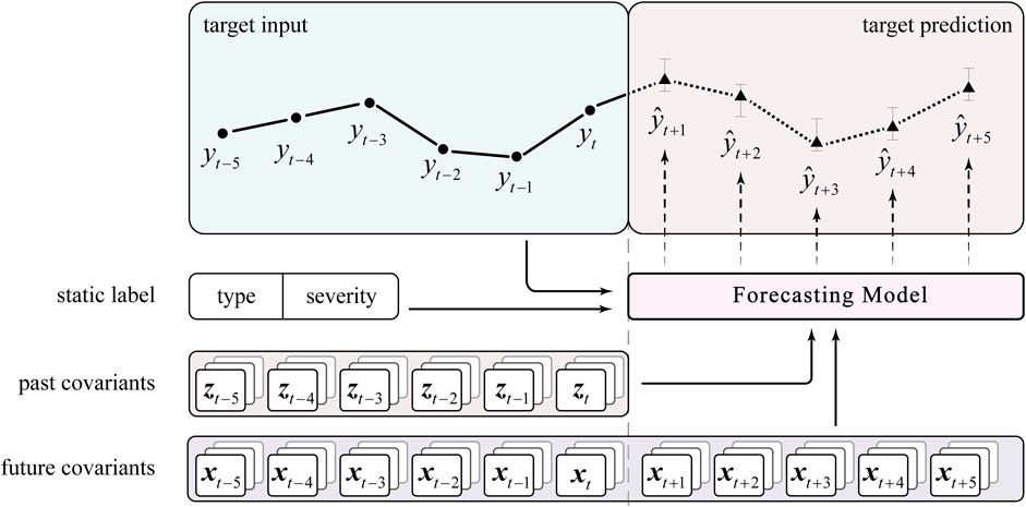
FIGURE 2. The visual description of the multi-horizon prediction problem for post-LOCA.
Temporal Fusion Transformers (TFT) present an advanced framework for time series forecasting that utilizes self-attention mechanisms to enhance prediction accuracy and offer interpretability in certain scenarios. This framework outperforms standard benchmarks, such as ARIMA, LSTM, and GRU, as well as more intricate models like DeepAR, MQRNN, and ConvTrans, in tests on open-source datasets (Lim et al., 2021). Overall, in the task of parameter prediction after LOCA of the reactor, TFT possesses five main technical features that ensure its excellent performance on the multi-horizon prediction problem, namely: 1) Use of gating mechanism: In the process of traversing the visible temporal dynamics, the gating mechanism can filter out irrelevant data points to reduce their interference with the prediction. 2) Input variable embedding module: In each time step, this module is able to embed a tiled vector of multiple covariates and known target variables into a fixed dimensional vector to facilitate the transfer of data in the model. 3) Static covariate encoder: this session will make full use of the accident diagnosis information, converting accident category labels and scalar labels into conditional information that constrains the calculation of each prediction step. 4) Dual temporal dynamic processing: On the one hand, LSTM is used to process the temporal data using sequence-to-sequence (Seq2Seq) approach to capture the data features of the data under short period; on the other hand, the distant relationships and features of the temporal data are captured using the Transformer layer based on the multi-headed self-attention mechanism, which thoroughly improves the long-term dependency problem in the traditional Seq2Seq. 5) Forecast range estimation: The quantile regression forecasting method is used to determine the possible range of target parameter values for each forecast time step. The flow of the prediction using the TFT model is shown in Figure 3.

FIGURE 3. A framework for multi-covariate prediction using TFT models.
A gated residual network (GRN) is employed to enhance the flexibility of the prediction model when the connection between input time series data and forecasted outputs is initially unclear. This approach selectively emphasizes data with notable correlations for input into the network. GRN reads an embedding vector
where

FIGURE 4. Calculation flow of GRN module.
Discrepancies in the quantity of historical and future covariates, along with static covariates, result in varying input vector dimensions at each temporal stage. To maintain dimensional consistency for downstream modeling, embedding is required to standardize the dimensions of these three covariate types at each time step. For any moment on the time axis, the covariates can be expressed as
This encoder receives the static covariate vector
where
The TFT employs a sequence-to-sequence (Seq2Seq) model with Long Short-Term Memory (LSTM) to identify key patterns in time series data, including trend shifts and notable fluctuations. It initializes with embeddings from static covariates and feeds historical and future covariate embeddings at each time step. This method outputs encoded information simultaneously for each time step, offering insights into the time series elements’ relative ordering. This approach moves beyond traditional fixed position encoding, providing a tailored inductive bias that enhances the prediction process for each step. For any moment
where
where
If all heads are considered, the average attention matrix
In the attention matrix
For the prediction range, the vector at each moment after multi-headed self-attention encoding can be denoted as
In this case, the different corner labels of GRN and GLU represent different network weights. Ultimately, the TFT’s point prediction is based on the calculation of the prediction interval, which is achieved by simultaneously predicting various percentiles, such as the 10th, 50th and 90th at each time step using a linear decoder. The calculation is shown in Eq. (14).
where
Based on the previous introduction of TFT, the structural features of the TFT prediction model mainly include gating mechanisms, variable embedding module, static covariate encoders, local and long-term temporal dynamics, and interval estimation. Compared with traditional prediction methods based on various deep learning models, such as classical LSTM or GRU, TFT has the following advantages for the prediction task of key parameters after LOCA:
1) To address the issue of memory retention in time series analysis, traditional approaches often relied on recurrent neural networks (RNNs), which incrementally process new inputs and consequently update the model’s short-term memory. This method, unfortunately, leads to a gradual diminishment of the effect of earlier data, which can cause increasing predictive errors over time. While advanced mechanisms like Long Short-Term Memory (LSTM) and Gated Recurrent Units (GRUs) introduce improvements for short-term memory extension, they fall short in fully addressing long-range dependencies. The Temporal Fusion Transformer (TFT) overcomes this limitation by utilizing an enhanced version of LSTM combined with a sophisticated multi-headed self-attention mechanism. This design allows the model to maintain a comprehensive perspective and retain earlier input data effectively.
2) The TFT enhances the effective use of information for forecasting by embedding features of data at each time step, which strengthens the extraction of relevant features. It employs a GRN to filter out less important data, like noise, and emphasizes key moments that are critical for accurate predictions, such as significant shifts or trends. Additionally, the TFT can process various types of data, including static covariates like incident categories and severity levels. This capability facilitates the integration of diagnostic and prognostic phases post-LOCA (Loss of Coolant Accident), overcoming the disconnect between these stages.
3) The prediction accuracy in critical safety situations is improved by using quantile regression to estimate uncertainty. This approach gives reactor operators a clearer understanding of the potential best and worst outcomes for the system’s response, rather than a single prediction at one time point. Accurately calculating uncertainty is vital in high-stakes safety environments.
This paper builds the TFT model as described and then uses it to forecast crucial parameters following a LOCA incident, assessing and enhancing the model’s performance. The workflow used in this paper is shown in Figure 5.
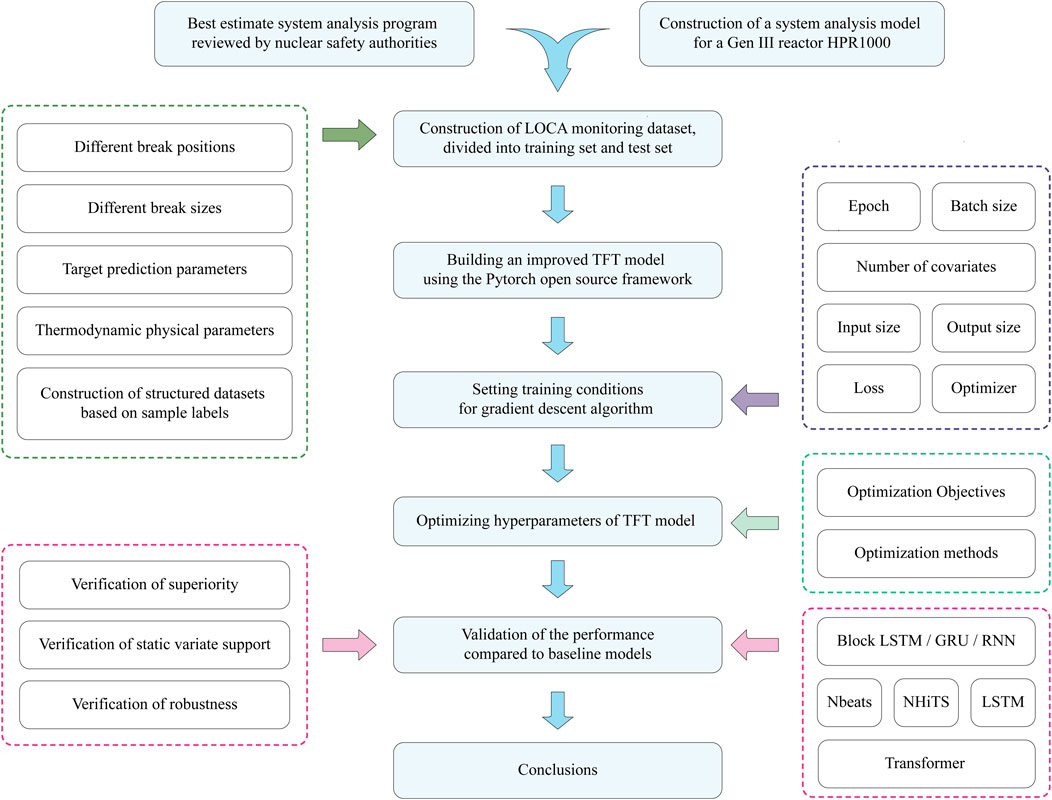
FIGURE 5. Flow chart of accident process prognosis after LOCA using TFT model.
When a LOCA occurs in a reactor, the operator needs to go through five steps to complete the treatment of the incident: data collection, anomaly sensing, incident diagnosis, status prognosis, and finally mitigation decision (Zhao et al., 2021). Condition prognosis directly serves the subsequent mitigation decisions and is therefore a link directly related to the success or failure of incident management. Currently, operators use emergency operating procedures (EOPs) constructed during the reactor design phase in the event of a LOCA. However, the accident transients on which the EOP is based are only a few sparse design conditions with severe consequences, and cannot cover real-world scenarios that may occur. This can lead to a tendency for the operator to use the most conservative approach even in less severe transient situations, resulting in an unnecessary waste of resources, even if the conservative process does not effectively envelop the transient. Therefore, in order to construct an accident process prognosis method that can be used at different breach locations and breach sizes, a dataset for training the TFT model needs to be constructed. Considering that no real-world data on LOCA transients are available, it is necessary to simulate the LOCA process for different initiation conditions using suitable tools.
This paper uses a pressurized water reactor system analysis program, Advanced Reactor System Analysis Code (ARSAC), developed by the Nuclear Power Institute of China (NPIC). ARSAC is a modern pressurized water reactor transient analysis program that solves a non-equilibrium non-homogeneous Eulerian-Eulerian six-equation two-phase fluid model using a gas-liquid two-phase model framework. The development of ARSAC follows the standard six steps of program development, namely requirements analysis, physical model study, software design, coding, testing, verification and validation (Deng et al., 2021). At present, ARSAC has been applied to several international benchmark problems, such as re-inundation experiments FLECHT-SEASET and other separation effect experiments, and large, middle and small breach loss of coolant accidents and other accident transient overall effect experiments, and the validation results show that the deviation of key parameters calculated by the ARSAC program from the experimental data is within a reasonable range. Therefore, the LOCA transients calculated using ARSAC are credible and reflect the reactor system response under realistic scenarios.
HPR1000 is a Gen III advanced nuclear power technology developed by China National Nuclear Corporation (CNNC) with a combined active and passive safety design concept. On the one hand, it is an evolutionary design based on the proven technology of existing pressurized water reactor nuclear power plants; on the other hand, it incorporates advanced design features, including 177 fuel assembly cores loaded with CF3 fuel assemblies, active and passive safety systems, comprehensive severe accident prevention and mitigation measures, enhanced protection against external events, and improved emergency response capabilities (Xing et al., 2016). Some of the key technical parameters used in the simulation of different LOCA initiation conditions for HPR1000 are shown in Table 1. As well, at the moment when the transient occurs, the system analysis program runs at the steady state of the rated power.

TABLE 1. Some of the key technical parameters of HPR1000 at the onset of LOCA transients.
In order to construct input cards that can be read by ARSAC, it is necessary to model the first loop and part of the second loop of the HPR1000, i.e. to illustrate the parameters of each reactor component and the connection relationships between the components, which is a process that can be represented in the form of a node diagram. The final node diagram of the HPR1000 reactor used to simulate the LOCA transient is shown in Figure 6, which contains the core of the reactor, the pressurizer, and key equipment on the three loops, such as the main pump and steam generator, as well as the main feedwater and steam co-tank of the second loop and the steam turbine for power generation.
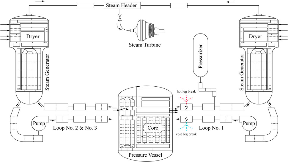
FIGURE 6. HPR1000 node diagram for simulating LOCA transients.
In order to simulate different LOCA initiation conditions, two main settings were made: 1) firstly, it was determined that the cold leg breach occurred at the connection between the two nearest pipe nodes before the coolant inlet from the core in the first loop, and the hot leg breach occurred at the connection between the two nearest pipe nodes after the coolant exit from the core in the same loop; 2) secondly, the breach size started with an equivalent diameter equal to 0.1 cm, and the step length is 0.2 cm, and ends at an equivalent diameter of 35.5 cm. The reason for setting different breach locations in the first place is mainly due to two considerations: 1) on the one hand, since there is always coolant flowing through the core compared to a hot leg breach, while a larger cold leg breach will result in a completely exposed core, the cold leg breach is the object of analysis in the reactor SAR, so the blind spot of the hot leg breach needs to be filled in the prognostic task for LOCA; 2) on the other hand, since the cold or hot leg is a category-based variable, it will help to extend the prognostic task to more accident category labels in the future. And the reason for setting more break sizes as an initiation condition is that compared to the large breaks where a dramatic system response occurs, small and middle breaks, although resulting in a less significant pressure relief process, still have the potential for complete core exposure, thus threatening the core integrity.
In the simulation of the LOCA cases, the simulation duration of each initiation event in this paper is 2000 s, and the state of the reactor at the current moment is recorded with a sampling frequency of twice per second. In the process of collecting covariates that contribute to the prediction of target parameters, this paper extracts 8 monitorable synthetic signals, and 22 direct signals, based on the physical signals that can be monitored by the actual instrumentation and control system of the HPR1000. The parameter identification and their corresponding physical significances are presented in Table 2. Synthetic signals, derived from direct signals indicative of the reactor’s systemic state, serve as suitable predictors for modeling tasks.
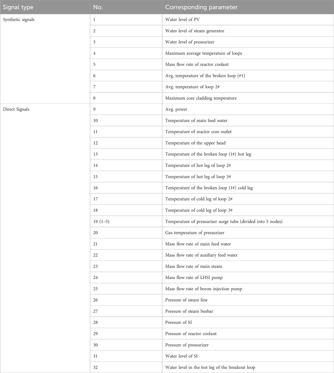
TABLE 2. Correspondence of Signal numbers and parameters monitored by instrumentation and control system.
Take the example of a middle break in the HPR1000 with a cold leg break size of 7.5 cm. Throughout the accident sequence, significant gas-liquid stratification of the reactor coolant system (RCS) occurs and there are two fuel temperature rises by gravity, which may lead to localized fuel damage. The first temperature rise is due to a loop water seal caused by the low point of the first loop system including the U-shaped elbow in front of the main pump and the lower part of the PV. This water seal causes the steam space to grow and the core to become exposed. When the break in the cold leg is exposed, the loop water seal at the low position of the reactor is removed, so the coolant is quickly re-entered into the core by the driving pressure head. The second temperature rise is caused by simple evaporation from the core. When the core is suddenly cooled due to the entry of new coolant, an early imbalance between the break flow and the safety injection flow can lead to a further drop in the PV water level, resulting in another bare core. The changes of the main synthetic monitoring signals after the occurrence of the middle break are shown in Figure 7. In the spray release phase, the PV water level signal decreases rapidly until the input of the position an injection box around 400 s; then, due to the formation of the loop water seal and the exposure of the core, the maximum temperature of the core envelope rises rapidly around 900 s; after 1600 s the loop water seal is lifted and the core water level rises again, at which time the maximum temperature of the envelope also starts to decrease.
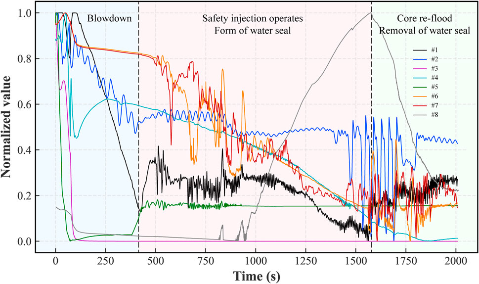
FIGURE 7. Variation of some key parameters in a typical cold leg middle break accident in 2000 s time.
To reduce the computational complexity of the training process, the input to the TFT model can be simplified by reducing the number of covariates with high similarity. In this paper, the correlation between each pair of reactor signals is analyzed using Pearson’s algorithm to obtain the signal correlation matrix including time and unmeasurable parameters, as shown in Figure 8. It can be seen that there are a large number of coefficients with correlations close to 1. Therefore, the coefficients are filtered by manual means. The trimmed coefficients are framed in red solid lines on the left side of the Figure 8.
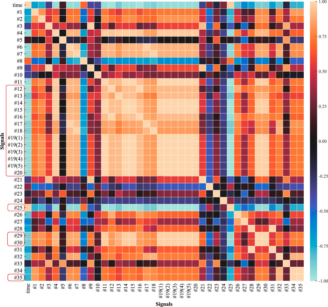
FIGURE 8. Heat map of Pearson correlation coefficients between pairs of reactor monitoring signals, and direct monitoring signals removed due to information redundancy.
In order to train the TFT model, an explicit differentiable optimization objective, i.e., a loss function, is needed first. In order to meet the requirements of the TFT prediction model for interval estimation, it is necessary to use an aggregated quantile residual as a loss function and the aggregation is additive, so that it is calculated as Eqs (15)–(16).
where
In the training process, the optimization method used is the Adam gradient descent optimizer. Adam has the advantages of the gradient descent algorithm with adaptive learning rate and the momentum gradient descent algorithm, which can improve the problem of prone to fall into the local minima of the loss function space while having a faster training speed. For the selection of the optimizer parameters, the initial learning rate is set to
In terms of data organization for the training process, all LOCA simulation databases are first partitioned into an 80% proportion of the training set and a 20% proportion of the test set. Then, the historical and prognostic data of each LOCA case are divided. The starting point of the prognosis is 100 s, which is due to the time consumed in order to undertake the diagnosis task of the accident (Li et al., 2022), i.e., the initiating parameters of the transient are identified using the diagnostic model within 100 s of the transient occurrence, and at this point all known information is used to further predict the trend of the parameter of interest between 100 and 2000 s. Finally, in the actual training process, the small batch gradient descent method is used because if all the training data are input into the GPU memory at one time, it will lead to memory overflow; if only one sample is used to update the gradient at a time, i.e., random gradient descent, it will lead to a decrease in the convergence speed of the model. The data organization of all LOCA cases for the TFT model training and testing process is shown in Figure 9.
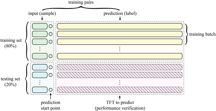
FIGURE 9. LOCA transient data organization for TFT model training and testing process.
The TFT model, being a complex deep neural network, has many hyperparameters linked to its structure. However, since optimizing all of them is not feasible, we focus on tuning those most crucial to prediction performance, based on the network’s key architectural features. The hyperparameters to be optimized and their alternative parameter search ranges are shown in Table 3.
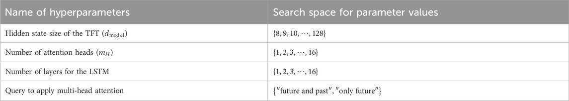
TABLE 3. The hyperparameters of the TFT model to be optimized and its search space.
We selected hyperparameters to ensure fast training and strong fitting for our model without needing to optimize on the entire dataset. We assessed the model on a small, random set of 10 LOCA cases with break diameters from 6.5 to 10.5 cm to pick the best hyperparameters. Given the high accuracy and confidence needed for post-LOCA predictions, we focused on two key metrics: the mean and variance of the residual distribution between the predicted and actual parameters at the 50% quantile should be as close to zero as possible, and the actual parameter values should mostly fall within the 10% and 90% prediction quantiles. Therefore, the optimization problem with hyperparameters can be defined as Eq. (17).
where
In this paper, we use a Bayesian optimization (BO) approach called Expected Improvement (EI) (Mockus, 1975) for the selection of hyperparameters. BO consists of two main elements: 1) the first component is a probabilistic agent model, which consists of a prior distribution and an observation model describing the data generation mechanism, such as a Gaussian process or a probabilistic tree model, and the observation model used in this paper is the Probabilistic Random Forest model; 2) the second component is an optimization objective, which describes a sequence of sampling and query processes to the best extent. The implementation algorithm for the single-objective optimization object of this paper is shown in Algorithm 1. The optimization iteration of hyperparameters is chosen to be 100 times, and the convergence curve of the optimization process is shown in Figure 10. Finally, the hyperparameters of the TFT network used for training are obtained as
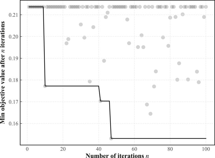
FIGURE 10. Convergence curves in hyperparameter optimization process.
Algorithm 1.Bayesian optimization (single target).
Input:
1:for
2: select new
3: obtain new observation
4: update trajectory container
5: update surrogate model
6:end
Output:
To assess the proposed reactor post-LOCA critical parameter prediction model using thin-film transistor technology (TFT), this study compares it with standard benchmarks and sophisticated deep learning algorithms. Model selection prioritizes high predictive precision and quantifiable confidence intervals in post-LOCA scenarios, adhering to these criteria:
(1) The prediction model is global rather than local. This means that the model can be tested on the training set and then can be directly inferred on the test set without further optimization of the model prior to inference (Lim and Zohren, 2021).
(2) The model is able to perform estimation of confidence intervals. That is, it is able to perform uncertainty estimation for the computational prediction step as the TFT model used in this paper.
(3) The model is capable of receiving historical covariates as input. Although the TFT model used in this paper is capable of receiving static, historical, and future covariates as inputs, the restriction on the types of covariates supported by the comparison model is relaxed, considering that historical covariates may contribute the majority of information in the forecasting process.
Considering the above requirements, the comparison models used in this paper contain NiHiTS (Challu et al., 2022), Nbeats (Oreshkin et al., 2020), Transformer (Shazeer, 2020), LSTM and Block-LSTM, GRU and Block-GRU, RNN and Block-RNN. The three neural network prediction models with “Block” prefixes are unique compared to the prefix-less models in that they use a fully connected network to produce a fixed-length output after encoding a fixed-length input block using a recurrent encoder, and therefore have a faster prediction speed.
In this paper, two synthetic monitoring parameters highly relevant to system safety are selected for prognosis: the PV water level and the average temperature of the coolant in the breakout loop. After training the TFT model using randomly selected time-series data as shown in Figure 9 and testing on some of the remaining data, the results of the predicted PV water level parameters under hot and cold leg LOCA are obtained as shown in Figures 11, 12, respectively; the prediction results of the average temperature of the break loop under hot and cold leg LOCA are shown in Figures 13, 14, respectively. Overall, although the prediction results using TFT have different degrees of lags at key turning points and locations of drastic changes, the confidence intervals are basically able to envelop the true parameter changes, indicating a high degree of confidence in the prediction results. In addition, the distributions of the residuals between the 50% quantile of the predicted and true simulated values of the two parameters are shown in Figures 15, 16, respectively. It can be seen that the residual variables roughly follow a Gaussian distribution and have a mean and variance close to zero, thus reflecting the high accuracy of the prognosis.
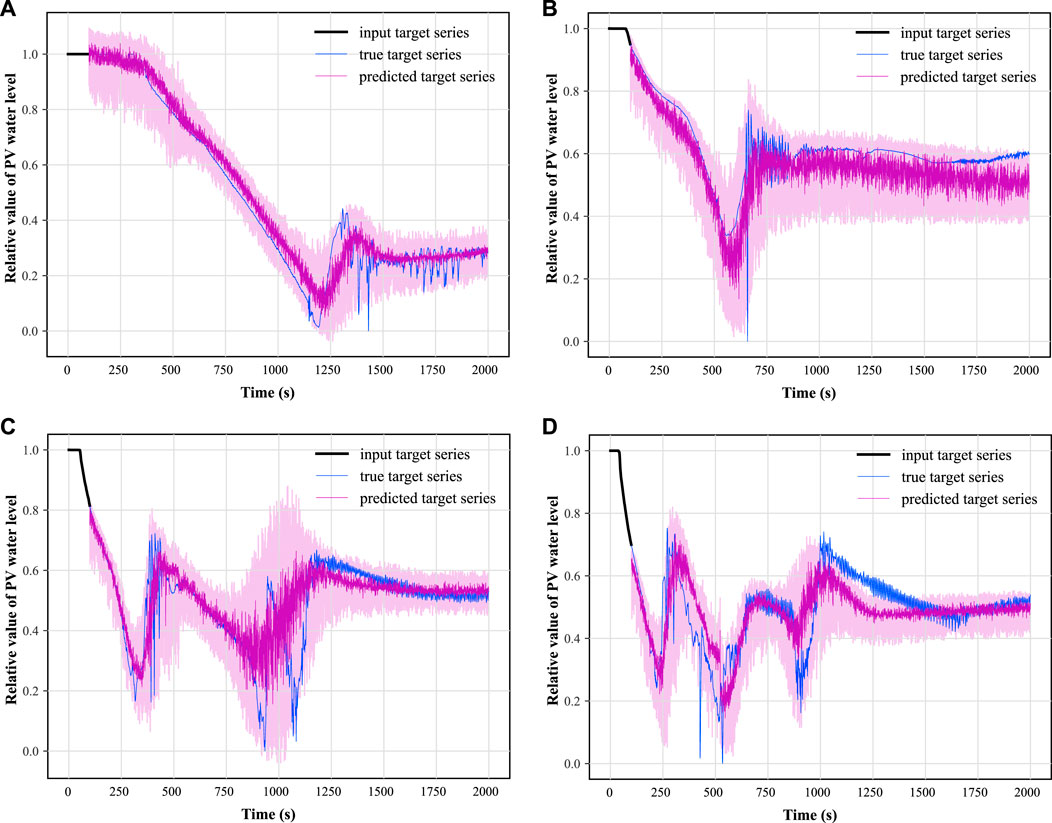
FIGURE 11. Samples of PV water level prognosis under hot leg LOCA.
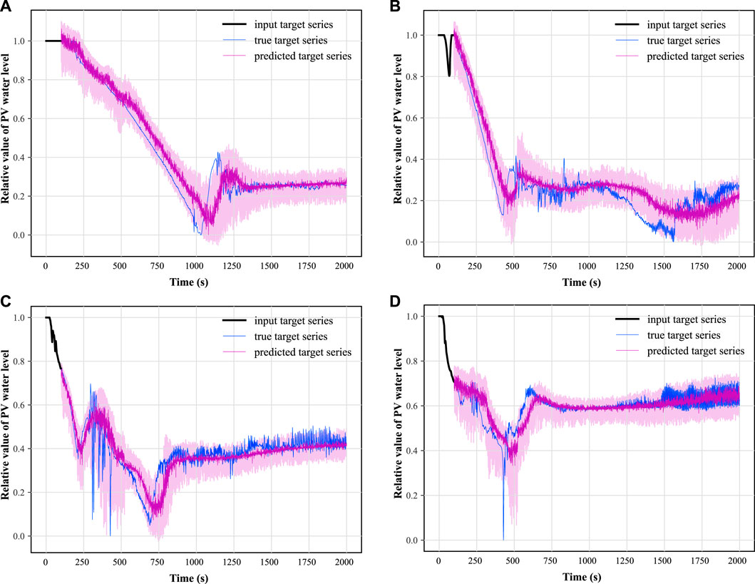
FIGURE 12. Samples of PV water level prognosis under cold leg LOCA.
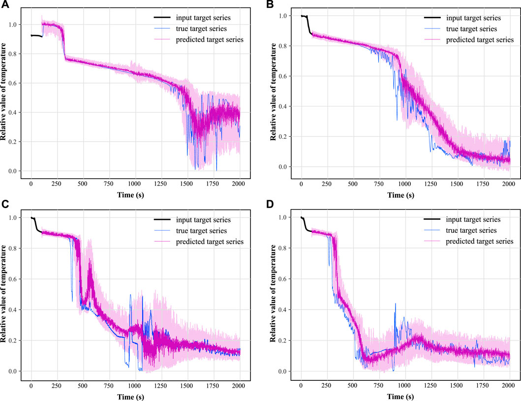
FIGURE 13. Samples of average temperature prognosis of the breaking loop under hot leg LOCA.
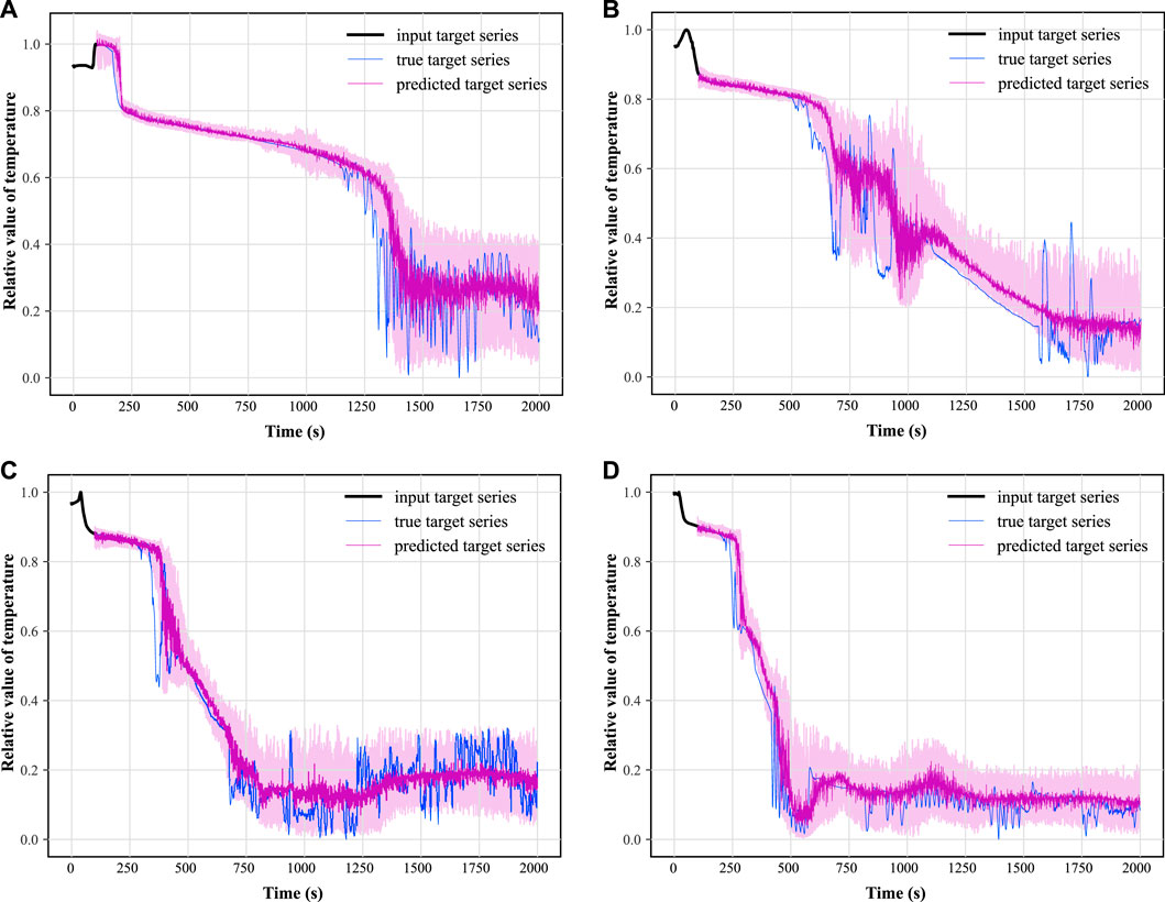
FIGURE 14. Samples of average temperature prognosis of the breaking loop under cold leg LOCA.
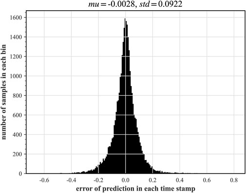
FIGURE 15. Distribution of PV water level prediction 50% quantile deviation from measured value.
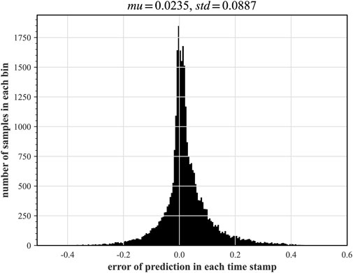
FIGURE 16. Distribution of deviations of the 50% quantile of the predicted value from the average temperature measurement of the breaking loop.
After obtaining the prediction results of the TFT model, the other prediction models used for comparison were trained with the same training method and the PV water level and the average temperature of the breach loop were predicted separately to obtain a comparative performance index of different prediction methods, and the performance pairs are shown in Table 4. Among the six specific evaluation metrics selected, the TFT model used in this paper obtained the highest performance in four of them. Therefore, it can be shown that the TFT model used in this paper is significantly superior for the task of prognosis of reactor accident parameters.
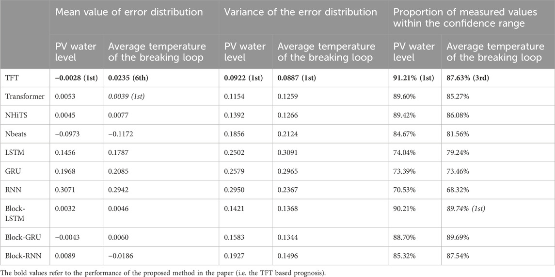
TABLE 4. Performance comparison of TFT models and different prognostic methods.
In LOCA, the pronounced pressure drop and two-phase flow spray induce rheological oscillations within the primary loop, compromising measurement precision at various points. Therefore, it is essential to assess the predictive accuracy of models under varying levels of noise interference. The object used for the evaluation process is the TFT model trained in Table 4, which relies on the training data as a result of the simulation of LOCA by the system analysis program without additional added noise. Since monitoring data from real LOCA scenarios are not available, the deviation distribution of model predictions after adding noise with different signal-to-noise ratios (SNR) to the sequence of historical target parameters and the sequence of historical covariates on which the model predictions depend will be analyzed. In this paper, we consider the case where the SNR levels are
The parameters of the bias distribution, i.e., the mean and variance, of the output of the prediction model using different SNRs are obtained with no changes to the static covariates and time variables, as shown in Figure 17. It can be seen that with the increase of noise, the variance of the prediction error of the water level signal and temperature signal does not show much change, and the absolute value of the prediction error of the temperature signal does not show large fluctuations. The only change that is more obvious is that the absolute value of the prediction error of the water level signal has a large increase with the increase of the SNR. After analysis, this is due to the existence of a wide range of low-frequency oscillation data characteristics of the water level in the middle LOCA range (e.g., Figures 11C, D), resulting in the TFT model in predicting the signal changes in this interval will pay more attention to the relative position information of the data points, making the predicted initial value more sensitive to the mean value of the error. Specifically seen is the predicted performance of the TFT for PV water level for size 10.5 cm hot leg LOCA at SNRs of 40.0 and 15.0, respectively, as shown in Figure 18.
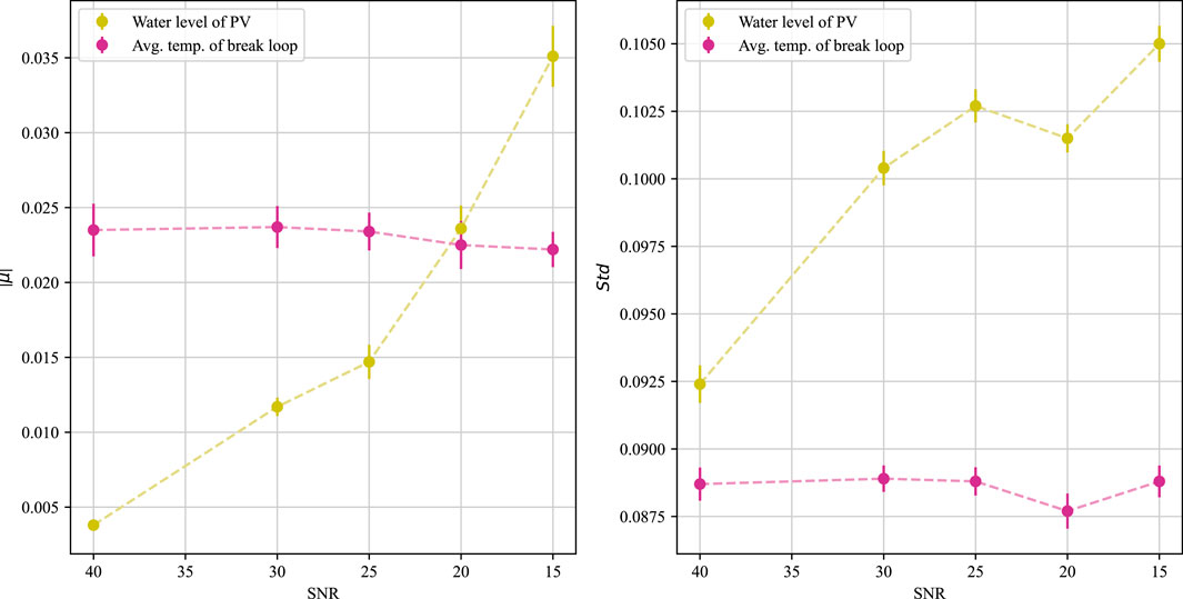
FIGURE 17. Prognostic performance of TFT models on test sets with different SNRs for input parameters.
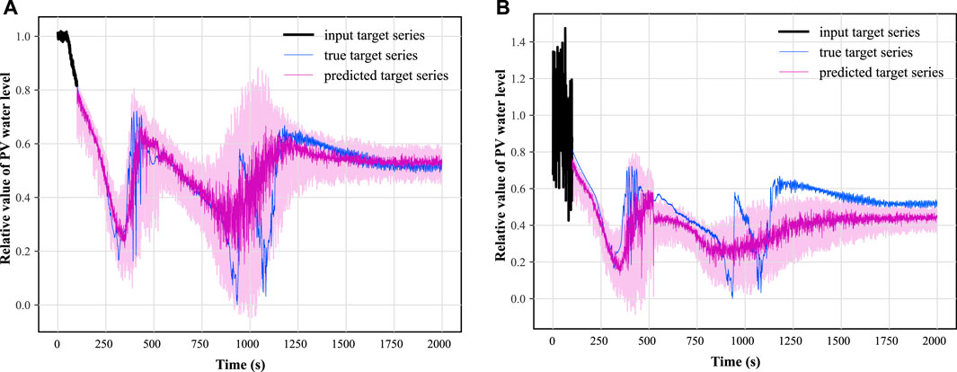
FIGURE 18. The performance of TFT model for PV water level prediction at SNR of 40.0 and 15.0.
To account for the robust performance of the TFT in the presence of noisy data, we propose two hypotheses: Firstly, the TFT discerns pertinent accident characteristics within the noisy inputs. Secondly, the inherent static features in the data inputs encapsulate ample accident-related information. To validate these propositions, we proceed with an ablation study on the static covariates, examining the TFT’s predictive accuracy across various SNRs while omitting details about the break’s location and magnitude. The experimental scheme consistent with the above section is used here to obtain the model prediction performance at each SNR value, as shown in Figure 19.
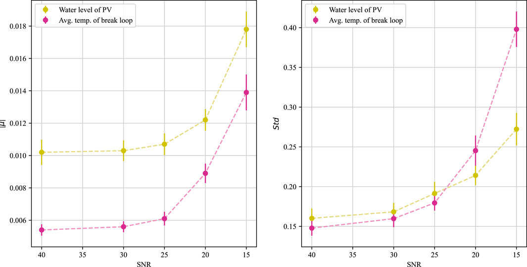
FIGURE 19. Prognostic performance of TFT models on the test set with different SNRs for input parameters under the condition of no static covariates.
The figure demonstrates that as noise increases, there is a marked rise in both the mean and variance of the error in predicted values. This occurs because, without the static covariates, the model relies solely on historical covariates for predictions, reducing the TFT’s capacity to accurately discern accident features under high noise conditions, confirming our initial hypothesis. Data with precise historical covariate details, which ensure correct accident diagnosis, maintain prediction accuracy even in noisy settings, as evidenced by comparing Figure 19; Figure 18. This observation aligns with our second hypothesis. In summary, the TFT model accommodates static covariates, thereby enhancing the robustness of prognosing the dynamics of accident processes.
This study proposed a Temporal Fusion Transformer (TFT) based method for multi-step prediction of critical parameters following reactor loss of coolant accidents (LOCAs). The TFT model utilizes multi-headed self-attention and gating mechanisms to achieve accurate and high-confidence forecasts of the accident evolution.
The key conclusions are three-fold. Firstly, TFT demonstrated superior accuracy and confidence interval estimation compared to current deep learning predictors. Secondly, robust extraction of valid accident features was evidenced under high noise scenarios through static covariate support. Thirdly, the integrated utilization of static and historical covariates improved data efficiency.
Limitations remain in prediction lag at key points and model robustness in real scenarios. Future coupling with diagnosis and online deployment could enable end-to-end diagnosis-prognosis optimization.
In summary, this research proposes a novel data-driven methodology for post-accident prognosis of reactor parameters. The TFT model offers nuclear operators robust support for accident management through enhanced prediction accuracy and confidence. Further verification on physical facilities would fully validate the practical utility.
The raw data supporting the conclusion of this article will be made available by the authors, without undue reservation.
CL: Writing–original draft. ML: Writing–review and editing. ZQ: Writing–review and editing.
The author(s) declare that no financial support was received for the research, authorship, and/or publication of this article.
The authors declare that the research was conducted in the absence of any commercial or financial relationships that could be construed as a potential conflict of interest.
All claims expressed in this article are solely those of the authors and do not necessarily represent those of their affiliated organizations, or those of the publisher, the editors and the reviewers. Any product that may be evaluated in this article, or claim that may be made by its manufacturer, is not guaranteed or endorsed by the publisher.
Allison, C. M., and Hohorst, J. K. (2010). Role of RELAP/SCDAPSIM in nuclear safety. Sci. Technol. Nucl. Installations 2010, 1–17. doi:10.1155/2010/425658
Ayodeji, A., Liu, Y., and Xia, H. (2018). Knowledge base operator support system for nuclear power plant fault diagnosis. Prog. Nucl. Energy 105, 42–50. doi:10.1016/j.pnucene.2017.12.013
Ayo-Imoru, R. M., and Cilliers, A. C. (2018). A survey of the state of condition-based maintenance (CBM) in the nuclear power industry. Ann. Nucl. Energy 112, 177–188. doi:10.1016/j.anucene.2017.10.010
Ba, J. L., Kiros, J. R., and Hinton, G. E. (2016). Layer normalization. Available at: https://arxiv.org/abs/1607.06450.
Challu, C., Olivares, K. G., Oreshkin, B. N., Garza, F., Mergenthaler-Canseco, M., and Dubrawski, A. (2022). N-HiTS: neural hierarchical interpolation for time series forecasting. Available at: https://arxiv.org/abs/2201.12886.
Deng, J., Ding, S., Li, Z., Huang, T., Wu, D., Wang, J., et al. (2021). The development of ARSAC for modeling nuclear power plant system. Prog. Nucl. Energy 140, 103880. doi:10.1016/j.pnucene.2021.103880
Encalada-Dávila, Á., Puruncajas, B., Tutivén, C., and Vidal, Y. (2021). Wind turbine main bearing fault prognosis based solely on scada data. Sensors 21, 2228. doi:10.3390/s21062228
Gao, Z., and Liu, X. (2021). An overview on fault diagnosis, prognosis and resilient control for wind turbine systems. Processes 9, 300. doi:10.3390/pr9020300
Gurgen, A. (2021). Development and assessment of physics-guided machine learning framework for prognosis system. North Carolina: University library in Raleigh.
Hong, J., Wang, Z., and Yao, Y. (2019). Fault prognosis of battery system based on accurate voltage abnormity prognosis using long short-term memory neural networks. Appl. Energy 251, 113381. doi:10.1016/j.apenergy.2019.113381
Hu, G., Zhou, T., and Liu, Q. (2021). Data-driven machine learning for fault detection and diagnosis in nuclear power plants: a review. Front. Energy Res. 9, 663296. doi:10.3389/fenrg.2021.663296
Jiang, B. T., Zhou, J., and Huang, X. B. (2020). Artificial neural networks in condition monitoring and fault diagnosis of nuclear power plants: a concise review. Int. Conf. Nucl. Eng. doi:10.1115/ICONE2020-16334
Koo, Y. D., An, Y. J., Kim, C.-H., and Na, M. G. (2019). Nuclear reactor vessel water level prediction during severe accidents using deep neural networks. Nucl. Eng. Technol. 51, 723–730. doi:10.1016/j.net.2018.12.019
Lee, G., Lee, S. J., and Lee, C. (2021). A convolutional neural network model for abnormality diagnosis in a nuclear power plant. Appl. Soft Comput. 99, 106874. doi:10.1016/j.asoc.2020.106874
Lei, Y. (2020). Applications of machine learning to machine fault diagnosis: a review and roadmap. Mech. Syst. Signal Process. 39. doi:10.1016/j.ymssp.2019.106587
Li, C., Qiu, Z., Yan, Z., and Li, M. (2022). Representation learning based and interpretable reactor system diagnosis using denoising padded autoencoder. Available at: https://arxiv.org/abs/2208.14319.
Li, J., and Lin, M. (2021). Ensemble learning with diversified base models for fault diagnosis in nuclear power plants. Ann. Nucl. Energy 158, 108265. doi:10.1016/j.anucene.2021.108265
Li, Y., Chen, C., Xin, P., Chen, Y., and Hou, H. (2017). “The gen-III nuclear power technology in the world,” in Proceedings of the 20th pacific basin nuclear conference. Editor H. Jiang (Singapore: Springer), 321–328. doi:10.1007/978-981-10-2314-9_27
Lim, B., Arık, S. Ö., Loeff, N., and Pfister, T. (2021). Temporal Fusion Transformers for interpretable multi-horizon time series forecasting. Int. J. Forecast. 37, 1748–1764. doi:10.1016/j.ijforecast.2021.03.012
Lim, B., and Zohren, S. (2021). Time-series forecasting with deep learning: a survey. Phil. Trans. R. Soc. A 379, 20200209. doi:10.1098/rsta.2020.0209
Lin, L., Athe, P., Rouxelin, P., Avramova, M., Gupta, A., Youngblood, R., et al. (2021). Development and assessment of a nearly autonomous management and control system for advanced reactors. Ann. Nucl. Energy 150, 107861. doi:10.1016/j.anucene.2020.107861
Liu, J., Vitelli, V., Zio, E., and Seraoui, R. (2015). A novel dynamic-weighted probabilistic support vector regression-based ensemble for prognostics of time series data. IEEE Trans. Reliab. 64, 1203–1213. doi:10.1109/TR.2015.2427156
Liu, Z., Zhang, Z., Li, D., Liu, P., and Wang, Z. (2022). “Battery Fault prognosis for electric vehicles based on AOM-ARIMA-LSTM in real time,” in 2022 5th International Conference on Energy, Electrical and Power Engineering (CEEPE). Presented at the 2022 5th International Conference on Energy, Electrical and Power Engineering (CEEPE), Chongqing, China, April 22-24, 2022, 476–483. doi:10.1109/CEEPE55110.2022.9783248
Ma, J., and Jiang, J. (2011). Applications of fault detection and diagnosis methods in nuclear power plants: a review. Prog. Nucl. energy 53, 255–266. doi:10.1016/j.pnucene.2010.12.001
Maitloa, A. A., Liua, Y., Lakhanb, M. N., Razac, W., Sharb, A. H., Alic, A., et al. (2020). Recent advances in nuclear power plant for fault detection and diagnosis-a review. J. Crit. Rev. 7, 4340–4349.
Mockus, J. (1975). “On the bayes methods for seeking the extremal point,” in IFAC Proceedings Volumes, 6th IFAC World Congress (IFAC 1975) - Part 1: Theory, Boston/Cambridge, MA, USA, August 24-30, 1975, 428–431. 8. doi:10.1016/S1474-6670(17)67769-3
Oreshkin, B. N., Chapados, N., Carpov, D., and Bengio, Y. (2020). N-BEATS: neural basis expansion analysis for interpretable time series forecasting 31. Available at: https://arxiv.org/abs/1905.10437.
Ramuhalli, P., Walker, C., Agarwal, V., and Lybeck, N. (2020). Development of prognostic models using plant asset data (No. ORNL/TM--2020/1697, 1661211). doi:10.2172/1661211
Saidi, L., Ben Ali, J., Bechhoefer, E., and Benbouzid, M. (2017). Wind turbine high-speed shaft bearings health prognosis through a spectral Kurtosis-derived indices and SVR. Appl. Acoust. 120, 1–8. doi:10.1016/j.apacoust.2017.01.005
Shazeer, N. (2020). GLU variants improve transformer. Available at: https://arxiv.org/abs/2002.05202.
Si, X.-S., Wang, W., Hu, C.-H., and Zhou, D.-H. (2011). Remaining useful life estimation – a review on the statistical data driven approaches. Eur. J. Operational Res. 213, 1–14. doi:10.1016/j.ejor.2010.11.018
Wang, H., Peng, M., Wesley Hines, J., Zheng, G., Liu, Y., and Upadhyaya, B. R. (2019). A hybrid fault diagnosis methodology with support vector machine and improved particle swarm optimization for nuclear power plants. ISA Trans. 95, 358–371. doi:10.1016/j.isatra.2019.05.016
Xing, J., Song, D., and Wu, Y. (2016). HPR1000: advanced pressurized water reactor with active and passive safety. Engineering 2, 79–87. doi:10.1016/j.eng.2016.01.017
Zeng, Y., Liu, J., Sun, K., and Hu, L. (2018). Machine learning based system performance prediction model for reactor control. Ann. Nucl. Energy 113, 270–278. doi:10.1016/j.anucene.2017.11.014
Zhang, J., Wang, X., Zhao, C., Bai, W., Shen, J., Li, Y., et al. (2020). Application of cost-sensitive LSTM in water level prediction for nuclear reactor pressurizer. Nucl. Eng. Technol. 52, 1429–1435. doi:10.1016/j.net.2019.12.025
Zhang, T., Chen, J., Li, F., Zhang, K., Lv, H., He, S., et al. (2022). Intelligent fault diagnosis of machines with small & imbalanced data: a state-of-the-art review and possible extensions. ISA Trans. 119, 152–171. doi:10.1016/j.isatra.2021.02.042
Zhao, X., Kim, J., Warns, K., Wang, X., Ramuhalli, P., Cetiner, S., et al. (2021). Prognostics and health management in nuclear power plants: an updated method-centric review with special focus on data-driven methods. Front. Energy Res. 9, 294. doi:10.3389/fenrg.2021.696785
Keywords: temporal fusion transformer, prognosis, loss of coolant accident, multi-horizon forecasting, HPR1000
Citation: Li C, Li M and Qiu Z (2024) A long-term dependable and reliable method for reactor accident prognosis using temporal fusion transformer. Front. Nucl. Eng. 3:1339457. doi: 10.3389/fnuen.2024.1339457
Received: 16 November 2023; Accepted: 15 January 2024;
Published: 07 February 2024.
Edited by:
Songbai Cheng, Harbin Engineering University, ChinaReviewed by:
Jinbiao Xiong, Shanghai Jiao Tong University, ChinaCopyright © 2024 Li, Li and Qiu. This is an open-access article distributed under the terms of the Creative Commons Attribution License (CC BY). The use, distribution or reproduction in other forums is permitted, provided the original author(s) and the copyright owner(s) are credited and that the original publication in this journal is cited, in accordance with accepted academic practice. No use, distribution or reproduction is permitted which does not comply with these terms.
*Correspondence: Meifu Li, bWVpZnVfbGVlQDE2My5jb20=
Disclaimer: All claims expressed in this article are solely those of the authors and do not necessarily represent those of their affiliated organizations, or those of the publisher, the editors and the reviewers. Any product that may be evaluated in this article or claim that may be made by its manufacturer is not guaranteed or endorsed by the publisher.
Research integrity at Frontiers
Learn more about the work of our research integrity team to safeguard the quality of each article we publish.