A probabilistic inverse prediction method for predicting plutonium processing conditions

In the past decade, nuclear chemists and physicists have been conducting studies to investigate the signatures associated with the production of special nuclear material (SNM). In particular, these studies aim to determine how various processing parameters impact the physical, chemical, and morphological properties of the resulting special nuclear material. By better understanding how these properties relate to the processing parameters, scientists can better contribute to nuclear forensics investigations by quantifying their results and ultimately shortening the forensic timeline. This paper aims to statistically analyze and quantify the relationships that exist between the processing conditions used in these experiments and the various properties of the nuclear end-product by invoking inverse methods. In particular, these methods make use of Bayesian Adaptive Spline Surface models in conjunction with Bayesian model calibration techniques to probabilistically determine processing conditions as an inverse function of morphological characteristics. Not only does the model presented in this paper allow for providing point estimates of a sample of special nuclear material, but it also incorporates uncertainty into these predictions. This model proves sufficient for predicting processing conditions within a standard deviation of the observed processing conditions, on average, provides a solid foundation for future work in predicting processing conditions of particles of special nuclear material using only their observed morphological characteristics, and is generalizable to the field of chemometrics for applicability across different materials.

1 Introduction to nuclear forensics

In 2011, the Department of Homeland Security (DHS) National Technical Nuclear Forensic Center (NTNFC) hosted a panel of Plutonium (Pu) experts to develop a plan for advancing forensic analysis of Pu materials. During this conversation, the experts concluded that different production processes produce final products with different characteristics. They hypothesized that these different characteristics, or “signatures”, on the final product could potentially allow a forensic analyst to determine which processes were used to produce the Special Nuclear Material (SNM), and, in turn, make inferences on where the material originated.

As a result of these discussions, scientists at Pacific Northwest National Laboratory (PNNL) conducted an experiment designed by statisticians at Los Alamos National Laboratory (LANL) and Sandia National Laboratories (SNL) to replicate historical and modern Pu processing methodologies and conditions. This experiment consisted of 76 runs, where each run considered the same set of nine processing parameters, whose values intentionally varied from run to run. For each run, the resulting SNM was imaged with a scanning electron microscope (SEM) to generate images of the various particles of Pu. These images were then segmented using LANL’s Morphological Analysis for Material Attribution (MAMA) software (Porter et al., 2016). This post-processing segmentation extracts the different particles that are present in each SEM image, and generates measurements based on the physical and morphological characteristics of the particles. Such measurements include particle areas, aspect ratios, convexities, circularities, gradients, and shadings (Zhang et al., 2021).

This paper serves to statistically relate the processing conditions of the different runs to the morphological and physical characteristics of the resulting Pu particles. In particular, we consider Pu particles that were processed using a solid oxalate feed, and particles that were processed in a 0.9 M oxalate solution. We relate the observed MAMA characteristics (which include, but are not limited to, those listed above) to the processing conditions used to produce the samples of Pu (which include, but are not limited to, temperature, nitric acid concentration, and Pu concentration) using inverse prediction methods. We consider Bayesian methodologies to quantify our predictions on the processing conditions, and to naturally incorporate uncertainty into these predictions.

We discuss these statistical methodologies in Section 2; in Section 3, we outline the specifics of the problem from a statistical perspective; in Section 4, we apply the methodologies to a dataset obtained from studying actual Pu particles generated under intentionally varied processing conditions within a design of experiments framework (rather than a simulated dataset); and in Section 5, we discuss the implications of our results.

2 An inverse prediction framework

To study the relationship between the processing parameters and the particle characteristics, we consider an inverse prediction framework. The traditional regression problem involves making predictions about responses, given a set of explanatory or input predictors. As a simple example, we may be interested in determining the weight of an individual, given their height, sex, and nationality. Conversely, the inverse prediction framework reverses the problem and so considers making predictions about the explanatory predictors, given a set of responses. Following the simple example above, we would now be interested in determining the height, sex and nationality of an individual, based on their weight. Inverse prediction is used across a variety of disciplines, and, in particular, has been used in forensic science, and nuclear forensics [see, for example, Lewis et al. (2018), Ries et al. (2018), and Ries et al. (2022)].

Mathematically, consider a q-dimensional response vector, $\mathit{y}={\left(y_1,y_2,\dots ,y_q\right)}^{\prime }$, and a p-dimensional input vector $\mathit{x}={\left(x_1,x_2,\dots ,x_p\right)}^{\prime }$. We express the relationship between x and y as

$\mathit{y}=g\left(\mathit{x}|\mathit{\theta }\right)+\epsilon ,(1)$

where $g\left(\cdot \right)$ is the true underlying physical phenomenon that is responsible for producing the results, which are typically represented by an emulator or surrogate that mimics the outputs in terms of the inputs, θ is a vector of model parameters, and ɛ is a random vector that captures noise present in the observed data.

As mentioned above, the goal of the inverse prediction framework is to predict the value of the input variables x′ that produced a new observation y′. There are two approaches by which we can learn about y′: We can either 1) construct a model that directly predicts x′ as a function of y′, or we can 2) invert a traditional forward model that predicts y′ as a function of x′. We will refer to the first approach as the “direct” model, and the second approach as the “inverse” model. It should be noted that, while it is more convenient to construct the “direct” model, this approach may violate regression assumptions. For example, standard linear regression models assume that the input variables are measured with negligible error. By constructing a model that directly predicts x′ as a function of y′, we are treating x as the output variable and y as the input variable and so this assumption no longer holds. Additionally, the “direct” model may not be well-suited for optimal design of experiments, since the vast majority of literature in design of experiments does not consider the inverse problem in its formulation (Anderson-Cook et al., 2015; Anderson-Cook et al., 2016).

In this paper, we use Bayesian Model Calibration (Kennedy and O’Hagan, 2001; Higdon et al., 2004, 2008; Walters et al., 2018; Lee et al., 2019; Nguyen et al., 2021) to approach the inverse prediction framework. Model calibration is a process to estimate, or calibrate, model parameters in the context of an input to output relationship, and falls under the second method (the “inverse” model) discussed above. More specifically, we are interested in using a calibration approach to make predictions about the processing conditions that were used to produce samples of Pu. Each of these samples consists of several particles whose morphological characteristics contain information pertaining to the conditions under which they were produced. By studying the information contained in these particles, we can infer the associated processing conditions.

In this paper, we use a fully Bayesian adaptive spline surfaces (BASS) framework to model or build an emulator to approximate the underlying relationship between the inputs and outputs (Francom et al., 2018; Francom et al., 2019; Francom and Sansó, 2020)¹. Suppose y is a vector of morphological characteristics associated with a sample of Pu, and x is a vector of processing conditions used to produce a sample of Pu. Without loss of generality, suppose that each x₁, x₂, …, x_p ∈ [0, 1]. The input to output relationship is modeled using.

$\mathit{y}=a_0+\sum _{m=1}^M{a}_m{B}_m\left(\mathit{x}\right)+\mathit{\epsilon },(2)$

where a₀ is the intercept, B_m(x) is a basis function on the input variables x, a_m is the coefficient for the mth basis function, and ɛ ∼ MVN(0, Σ) (Francom and Sansó, 2020). We consider priors for each of the parameters, a, σ², and M. Note that, because we define a prior over M, the number of basis functions is not fixed, and varies throughout the sampling process. These parameters are sampled using a Markov Chain Monte Carlo (MCMC) process. The samples obtained from this process constitute the posterior distribution of the input parameters, given the observed output parameters.

Upon defining the appropriate BASS model, we perform Bayesian Model Calibration, which allows us to estimate the input parameters that make the model best match the data provided by the output parameters. In this instance, we do not include a discrepancy term. Ideally, a discrepancy term would capture model bias error (i.e., how well a physical model approximates reality), which, in our case, is challenging to handle. Future work will include incorporating this discrepancy term, as well as exploring alternative emulators that are able to better capture the relationship between the input and the output parameters. For more details about Bayesian Model Calibration, see Kennedy and O’Hagan. (2001), Higdon et al. (2004), Higdon et al. (2008), Walters et al. (2018), and Nguyen et al. (2021).

3 Inverse prediction for Pu processing conditions

Suppose that run $r\in \left\{1,\dots ,R\right\}$ results in n_r images and L_r particles. The number of images varies between particles, and the number of particles varies between images, so that the number of particles per run is not consistent. For our data, R = 76. Each of the runs in our experiment yielded between 5 and 176 images per run, and between 81 and 4,643 particles per run. By using information contained in these runs, we can make predictions about the processing conditions of a new run. In this scenario, our input parameters include processing conditions such as temperature, nitric acid, and Pu concentrations, and responses include morphological characteristics such as particle shape and size.

Figure 1 demonstrates two different particles from two different runs, each with different processing conditions. Note that, while size and shape are useful for determining processing conditions of a sample, far more information is required to accurately predict the processing conditions of these two particles. For example, we can see that, while these particles are produced under entirely different processing conditions, they do maintain physical similarities, alluding to the difficulty of this problem. While both particles are made up of flat sheets, we can see that the arrangement of and the angles between these sheets do differ from one another. This information is captured by segmenting the particles using LANL’s MAMA software, which allows for capturing information about the morphological characteristics, such as area, diameter, and aspect ratio. By including the information from the MAMA software in our model, we can better distinguish between particles from different runs.

FIGURE 1

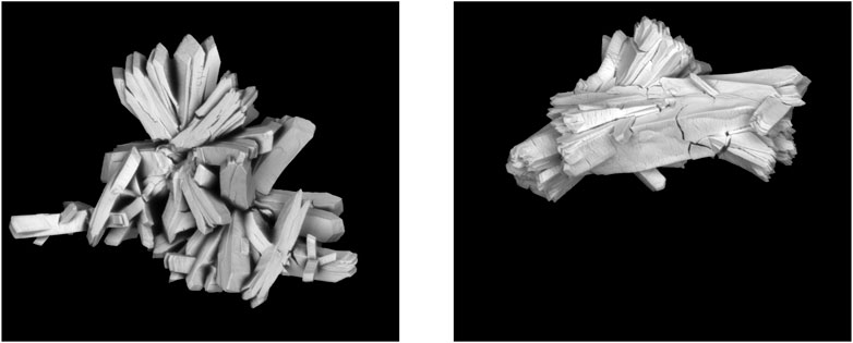
FIGURE 1. Examples of particle textures resulting from two different runs, with two different sets of processing conditions.

From Section 2, we have that y is a p-vector of morphological characteristics associated with a sample of Pu, and x is the q-vector of processing conditions used to produce that sample of Pu. Given our sample of L_r particles for each of our 76 runs, Y_r is the L_r × p matrix of morphological characteristics, where each row of Y_r corresponds to the morphological characteristics of the L_r particles associated with run r ∈ {1, …, 76}. Our full matrix of morphological characteristics is then given by the ${\sum }_{r=1}^{76}{L}_r\times p$ matrix Y, such that

$\mathit{Y}=\left[\begin{array}{c}\hfill {\mathit{Y}}_1\hfill \\ \hfill {\mathit{Y}}_2\hfill \\ \hfill ⋮\hfill \\ \hfill {\mathit{Y}}_R\hfill \end{array}\right]\text{where\hspace{0.17em}each\hspace{0.17em}}{\mathit{Y}}_r=\left[\begin{array}{c}\hfill {\mathit{y}}_{r1}\hfill \\ \hfill {\mathit{y}}_{r2}\hfill \\ \hfill ⋮\hfill \\ \hfill {\mathit{y}}_{r{L}_r}\hfill \end{array}\right]=\left[\begin{array}{cccc}\hfill y_{r11}\hfill & \hfill y_{r12}\hfill & \hfill \cdots \hfill & \hfill y_{r1p}\hfill \\ \hfill y_{r21}\hfill & \hfill y_{r22}\hfill & \hfill \cdots \hfill & \hfill y_{r2p}\hfill \\ \hfill ⋮\hfill & \hfill ⋮\hfill & \hfill \ddots \hfill & \hfill ⋮\hfill \\ \hfill y_{r{L}_{r}1}\hfill & \hfill y_{r{L}_{r}2}\hfill & \hfill \cdots \hfill & \hfill y_{r{L}_{r}p}\hfill \end{array}\right].$

As an example, consider row y_r2 in the matrix Y_r. This vector corresponds to the p observed morphological characteristics associated with the second particle in run r, so that y_r21 corresponds to the observed value for the first morphological characteristics for particle 2 in run r, y_r22 corresponds to the observed value for the second morphological characteristic for particle 2 in run r, and so on.

The matrix X is analogously defined for the processing conditions, where X_r is the L_r × q matrix of processing conditions, where each row of X_r is the q-vector of processing conditions associated with the corresponding run r. For dimensional consistency, we consider X_r as the L_r × q matrix, where x_r is merely repeated for each of the L_r rows in X_r, since all particles in run r are produced under the same set of processing conditions.

Before proceeding with calibration, we must first define our emulator. We choose to fit a BASS model using the associated BASS package in R (Francom and Sansó, 2020). We then perform model calibration to obtain the best set of processing conditions that are associated with a new set of observed morphological characteristics, captured by the matrix Y_R+1, that results from observing a set of particles from a new run.

Since run R+1 results in L_R+1 particles, we calibrate on each of the l_R+1 vectors of morphological characteristics. Each of these calibrations results in N_MCMC samples for each of the p processing conditions. That is, for a set of L_R+1 particles, we obtain L_R+1 N_MCMC × p matrices of predicted processing conditions, ${\mathit{X}}_{R+11},\dots ,{\mathit{X}}_{R+1L_{R+1}}$. We can use the results from this set of L_R+1 matrices to determine a point estimate, and highest posterior density intervals for the p processing conditions. This process is outlined in Algorithm 1.

4 Application

In this section, we apply the above methodology to our dataset. The data considered in this experiment consists of runs that were processed using two types of oxalate feed. Out of the 76 total runs, 24 of these runs were processed using a solid oxalate feed, and 52 were processed in 0.9 M oxalate solution. We analyze these two sets separately (Sections 4.1, 4.2), and jointly (Section 4.3). Considering the different types of runs separately and jointly allows us to study the effects of training models on data that are either a) more representative of an interdicted sample (i.e., when we consider the different types of oxalate feeds separately and train separate models for the different types of oxalate feeds), or b) trained on more data, and thus able to learn more (i.e., when we consider the different types of oxalate feeds together and train the model on the joint data). For example, classification techniques may allow us to distinguish between solid and solution runs. In this case, given a test run that we determine to be either a solid or solution run, we can train our model on runs that are more representative of the run we are studying.

4.1 Solid runs

In this section, we consider the 24 solid runs separately from the 76 total runs. We apply Algorithm 1 via a leave-one-out cross-validation (LOO-CV) process (Lachenbruch and Mickey, 1968; Luntz and Brailovsky, 1969; Gareth et al., 2013), in which we withhold all particles associated with a given run. That is, we treat the particles associated with a given run as our newly observed particles on which we wish to perform calibration.

To quantify the ability of the algorithm to successfully predict the processing conditions of a given run, we consider the Root Mean Square Error (RMSE) of the predicted value of the processing conditions compared to the observed value of the processing conditions. The RMSE is a useful quantity to consider, since it is robust to distribution specification, given that it is based on a point estimate, and has a nice interpretation, especially when the data being considered is normalized. As such, before training the models, we center and scale the values so that we can interpret the RMSEs in the context of standard deviations of the processing conditions. For example, RMSEs of less than one indicate that the predicted values are within one standard deviation of the true values, RMSEs of less than two indicate that the predicted values are within two standard deviations of the true values, and so on. Figures 2, 3 demonstrate the ability of this method to make predictions when we train our algorithm on solid runs, to predict processing conditions of particles produced by solid runs.

FIGURE 2

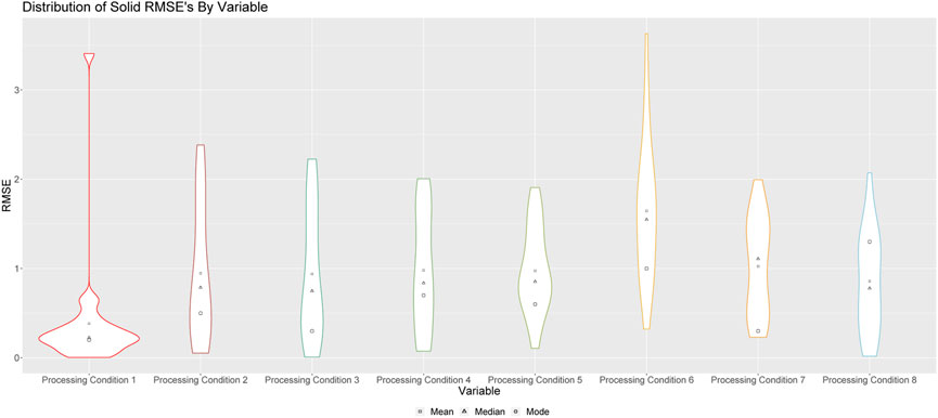
FIGURE 2. Violin plots of RMSEs for processing conditions 1 through 8 for solid runs. Square points represent the means of these distributions; triangular points represent the median of these distributions, and circular points represent the modes of these distributions.

FIGURE 3

FIGURE 3. Breakdown of RMSE by processing condition across solid runs. The height of a given column relays the overall RMSE for the associated run. Each color corresponds to the proportion of this RMSE that can be attributed to each processing condition.

Figure 2 shows the violin plots of RMSEs when the medians of the resulting empirical distributions of posterior modes is used as a point estimate. From a comprehensive study of the solid runs, we were able to determine that the median of the empirical distributions of the posterior modes served as the best point estimate of the true processing condition. This is also true for the studies completed in Sections 4.2, 4.3.

The results in Figure 2 indicate that the algorithm is better at predicting some processing conditions (which include conditions such as temperature, nitric acid concentration and Pu concentration) than others. For example, we see that, aside from processing conditions 3 and 5, this method is, on average, capable of predicting the processing conditions of a sample of Pu within a single standard deviation. In fact, the method is particularly effective at predicting processing conditions 1, 2 and 8, as is indicated by the modes of these distributions, which demonstrates that more often than not, our prediction for these processing conditions is within 0.5 standard deviations of the true value. We note that it is not particularly surprising that, in some instances, the RMSE can extend beyond a single standard deviation. Given that the production of a family of material types (in this case, Pu) requires a chemical expert to precisely execute a series of involved tasks, it is not particularly surprising using only the morphological characteristics of the end product can result in uncertainties on the predicted values of the processing conditions that extend past 3 RMSE. Whether an RMSE below 0.5 is acceptable is not a straightforward determination. Much like the level of significance, alpha, used in hypothesis testing, the threshold at which uncertainty is acceptable to the user is dependent on the objective at hand. If the uncertainty is deemed to be inadequate, then a reflection on how uncertainty can be decreased would likely be useful. This exercise provides insight not only for forensic purposes, but also for insights for biases and deviations from standard processes.

Figure 3 shows the proportional breakdown of RMSE by processing condition for each run. For each run, we see the proportion of the overall RMSE that can be attributed to each processing condition. The greater the difference in the widths of the colored bars, the more disparate their individual RMSEs are from one another, and from the overall RMSE. This helps us to determine which processing conditions are well predicted for a given run, and which processing conditions are poorly predicted for a given run. From this figure, we can see that the predictions within processing conditions are relatively consistent between runs.

As an example, consider run 22. We see that the RMSE across all processing conditions for Run 22 is approximately 1.7 (the overall height of the stacked bar). Within this bar, we can see how each individual processing condition contributes to the root average of 1.7 (the individual covered bars). For run 22, we see that the individual colored bars are made up of several different heights, indicating that the overall RMSE for run 22 is not representative of each processing condition’s individual RMSE. Since processing condition 1 and 8 are represented by very thin bars, their individual RMSE’s are much smaller than 1.7 (and, in fact, are actually close to zero). On the other hand, we see that processing condition 6 is represented by a much taller bar, indicating that its individual RMSE is much larger than 1.7. This large difference is offset by the much smaller values of RMSE for processing conditions 1 and 8 when we take the root mean of all squared errors for to obtain the overall RMSE.

4.2 Solution runs

In this section, we consider the 52 solution runs separately from the 76 total runs. As before, we apply Algorithm 1 via an LOO-CV process, and consider RMSEs to quantify the performance of our models. Figures 4, 5 demonstrate the ability of this method to make predictions when we train our algorithm on solution runs, to predict processing conditions of particles produced by solution runs.

FIGURE 4

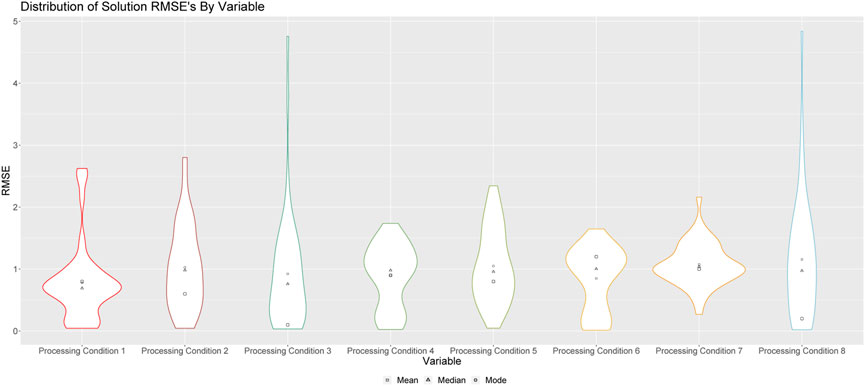
FIGURE 4. Violin plots of RMSEs for processing conditions 1 through 8 for solution runs. Square points represent the means of these distributions; triangular points represent the median of these distributions, and circular points represent the modes of these distributions.

FIGURE 5

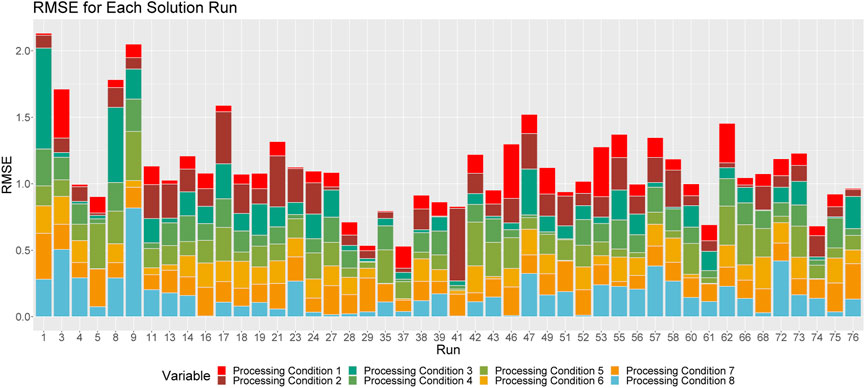
FIGURE 5. Breakdown of RMSE by processing condition across solution runs. The height of a given column relays the overall RMSE for the associated run. Each color corresponds to the proportion of this RMSE that can be attributed to each processing condition.

Figure 4 shows the violin plots of RMSE’s when the medians of the resulting empirical distributions of posterior modes is used as a point estimate. These results indicate that the algorithm is better at predicting some processing conditions than others. For example, we see that, aside from processing conditions 3 and 8, this method is, on average, capable of predicting the processing conditions of a sample of Pu within a single standard deviation. In fact, the method is particularly effective at predicting processing conditions 1 and 3, as is indicated by the modes of these distributions, which demonstrates that more often than not, our prediction for these processing conditions is within 0.5 standard deviations of the true value.

Figure 5 shows the proportional breakdown of RMSE by processing condition for each run. This figure demonstrates that the predictions within processing conditions are relatively consistent between runs.

4.3 All runs

In this section, we consider all 76 runs together. That is, the algorithm is trained on runs that were processed using a solid oxalate feed, as well as those that were processed in solution, regardless of whether the test run is a solid run or a solution run. As before, we apply Algorithm 1 via an LOO-CV process, and consider RMSEs to quantify the performance of our models. Figures 6, 7 demonstrate the ability of this method to make predictions when we train our algorithm on all runs, to predict processing conditions of particles produced by either a solid or solution run.

FIGURE 6

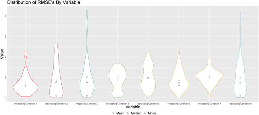
FIGURE 6. Distributions of predictions for processing conditions 1 through 8 for all runs. Square points represent the means of these distributions; triangular points represent the median of these distributions, and circular points represent the modes of these distributions.

FIGURE 7

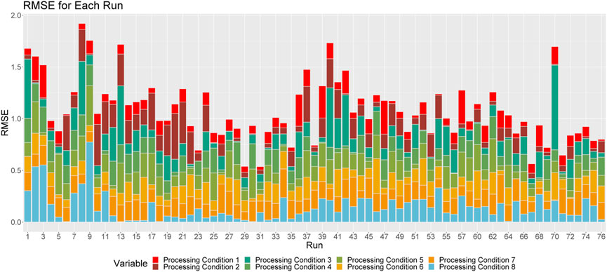
FIGURE 7. Breakdown of RMSE by processing condition across all runs. The height of a given column relays the overall RMSE for the associated run. Each color corresponds to the proportion of this RMSE that can be attributed to each processing condition.

Figure 6 shows the violin plots of RMSE’s when the medians of the resulting empirical distributions of posterior modes is used as a point estimate. Note that the shapes of these distributions are similar to those depicted in Figures 2, 4, indicating consistent prediction ability when we train on solid and solution runs together, versus training on just solid or just solution runs. We do note, however, that there are longer tails associated with these distributions, and that the overall RMSEs are larger when we train the algorithm on both solid and solution runs.

The results in Figure 6 indicate that the algorithm is better at predicting some processing conditions than others. For example, we see that, aside from processing conditions 3, 7 and 8, this method is, on average, capable of predicting the processing conditions of a sample of Pu within a single standard deviation. However, when we consider the mode as our point estimate, we see that the method is particularly effective at predicting processing conditions 1, 2, 4 and 8, as is indicated by the modes of these distributions, which demonstrates that more often than not, our prediction for these processing conditions is within 0.5 standard deviations of the true value.

Figure 7 shows the proportional breakdown of RMSE by processing condition for each run. This figure demonstrates that the predictions within processing conditions are relatively consistent between runs. Again, we see that the model is particularly apt at making predictions for processing conditions 1, 2, 4 and 8.

We also consider a direct comparison of the broken down RMSE by run when we train on the solution and solid runs separately and jointly. Figures 8, 9 show these relationships. By comparing these figures with Figures 3, 5, we can see how training on the solid and solution data jointly results in different predictions from those that result from training separate solid and solution models. In some instances, we see that the RMSE decreases, while in others, we see that it is increased, indicating that training a joint model is not necessarily worse than training two separate models. Furthermore, we see that the individual contribution of each processing condition to the overall RMSE for each run remains relatively consistent, although we do see slightly larger RMSEs for processing conditions 1 and 8 when we train jointly. In addition, we see that runs that are better predicted by the individually trained models are also better predicted by the jointly trained models for both solid and solution runs.

FIGURE 8

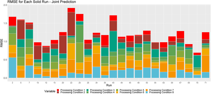
FIGURE 8. Breakdown of RMSE by processing condition across solid runs, when the model is trained on solid and solution data, jointly. The height of a given column relays the overall RMSE for the associated run. Each color corresponds to the proportion of this RMSE that can be attributed to each processing condition.

FIGURE 9

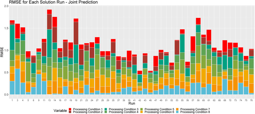
FIGURE 9. Breakdown of RMSE by processing condition across solution runs, when the model is trained on solid and solution data, jointly. The height of a given column relays the overall RMSE for the associated run. Each color corresponds to the proportion of this RMSE that can be attributed to each processing condition.

5 Conclusion

In this paper, we looked at the ability of a BASS model to predict the processing conditions of particles of Pu, given a set of morphological characteristics by Bayesian Calibration via a Bayesian Adaptive Spline Surface model. Not only does this model allow for providing point estimates of a sample of SNM, but it also incorporates uncertainty into these predictions. This model proved to be sufficient at predicting processing conditions within a standard deviation of the observed processing conditions on average, when applied to a dataset of particles of Pu. In particular, we found that this model is best able to predict processing conditions 1, 2, and 4, and struggles most with predicting processing conditions 3, 7, and 8. By comparing Figures 3, 5, 7, we see that using both solid and solution runs to train the model (versus analyzing solid and solution runs separately) does not affect the ability of the model to predict the processing conditions of a new run, indicating that the BASS model is flexible enough to incorporate this information into its predictions.

By predicting the processing conditions of samples of SNM, we can begin to understand where material may have been produced, or by whom. While it remains that this the results of this method should not be used as the sole evidence for reaching a forensic conclusion, this analysis demonstrates that statistical models can aid the nuclear forensic community. In particular, these models help provide insight into the various sources of uncertainty and bias in the chemical processes. In addition, they allow forensic decision makes to numerically bound their observations, and quantitatively support their inferences and predictions. Future studies will aim to improve these results by considering the effects of particle sizes on the predictions, and will incorporate functional shape and texture data. Additionally, we would like to determine whether incorporating the discrepancy term in our calibration step would allow us to further decrease the RMSE of our predictions. Nevertheless, this methodology provides a solid foundation for future work in predicting processing conditions of particles of SNM using only their morphological characteristics.

Data availability statement

The original contributions presented in the study are included in the article/supplementary materials, further inquiries can be directed to the corresponding author.

Author contributions

MA developed models, analyzed the data and compiled the manuscript. AM, DR, AZ, KS, KG, JT, and JH assisted with data analysis and manuscript review.

Funding

We acknowledge the Department of Homeland Security (DHS) Countering Weapons of Mass Destruction (CWMD) National Technical Forensics Center (NTNF), as well as the Office of Nuclear Detonation Detection (NA-222) within the Defense Nuclear Non-proliferation Research and Development of the US Department of Energy/National Nuclear Security Administration for funding this work at Los Alamos National Laboratory and at Sandia National Laboratories. This paper describes objective technical results and analysis.

Acknowledgments

We acknowledge the Department of Homeland Security (DHS) Countering Weapons of Mass Destruction (CWMD) National Technical Forensics Center (NTNF), as well as the Office of Nuclear Detonation Detection (NA-222) within the Defense Nuclear Non-proliferation Research and Development of the US Department of Energy/National Nuclear Security Administration.

Conflict of interest

The authors declare that the research was conducted in the absence of any commercial or financial relationships that could be construed as a potential conflict of interest.

Publisher’s note

All claims expressed in this article are solely those of the authors and do not necessarily represent those of their affiliated organizations, or those of the publisher, the editors, and the reviewers. Any product that may be evaluated in this article, or claim that may be made by its manufacturer, is not guaranteed or endorsed by the publisher.

Author disclaimer

Any subjective views or opinions that might be expressed in the paper do not necessarily represent the views of the US Department of Energy or the United States Government. Los Alamos National Laboratory strongly supports academic freedom and a researcher’s right to publish; as an institution, however, the Laboratory does not endorse the viewpoint of a publication or guarantee its technical correctness. Sandia National Laboratories is a multimission laboratory managed and operated by National Technology and Engineering Solutions of Sandia, LLC, a wholly owned subsidiary of Honeywell International, Inc., for the US Department of Energy’s National Nuclear Security Administration under contract DE-NA0003525. Approved for public release: LA-UR-21-25447.

Footnotes

¹The BASS framework is similar to the Bayesian multivariate adaptive regression splines (BMARS) framework developed by Denison et al. (1998) [see also Friedman (1991)], but with added features that promote efficiency in the sampling processes to allow for a more efficient model estimation (e.g., Reversible Jump Markov Chain Monte Carlo (RJMCMC) via Nott et al. (2005), parallel tempering). Like the BMARS framework, the BASS framework uses the input data to learn a set of basis functions that provide an approximate to $g\left(\mathit{x}|\mathit{\theta }\right)$ that, when considered together, give the best predictions of the output data. Like its BMARS counterpart, BASS is particularly well-suited for capturing non-linear relationships between the input and output variables (Francom and Sansó, 2020).

References

Anderson-Cook, C., Burr, T., Hamada, M., Ruggiero, C., and Thomas, E. (2015). Design of experiments and data analysis challenges in calibration for forensics applications. Chemom. Intelligent Laboratory Syst. 149 (B), 107–117. doi:10.1016/j.chemolab.2015.07.008

CrossRef Full Text | Google Scholar

Anderson-Cook, C., Hamada, M., and Burr, T. (2016). The impact of response measurement error on the analysis of designed experiments. Qual. Reliab. Eng. Int. 32 (7), 2415–2433. doi:10.1002/qre.1945

CrossRef Full Text | Google Scholar

Denison, D., Mallick, B., and Smith, A. (1998). Bayesian Mars. Statistics Comput. 8, 337–346. doi:10.1023/a:1008824606259

CrossRef Full Text | Google Scholar

Francom, D., and Sansó, B. (2020). Bass: An r package for fitting and performing sensitivity analysis of bayesian adaptive spline surfaces. J. Stat. Softw. 94 (8), 1–36. doi:10.18637/jss.v094.i08

CrossRef Full Text | Google Scholar

Francom, D., Sansò, B., Bulaevskaya, V., Lucas, D., and Simpson, M. (2019). Inferring atmospheric release characteristics in a large computer experiment using bayesian adaptive splines. J. Am. Stat. Assoc. 114 (528), 1450–1465. doi:10.1080/01621459.2018.1562933

CrossRef Full Text | Google Scholar

Francom, D., Sansó, B., Kupresanin, G., and Johannesson, G. (2018). Sensitivity analysis and emulation for functional data using bayesian adaptive splines. Stat. Sin. 28 (2), 791–816. doi:10.5705/ss.202016.0130

CrossRef Full Text | Google Scholar

Friedman, J. (1991). Multivariate adaptive regression splines. Ann. Statistics 19 (1), 1–67. doi:10.1214/aos/1176347963

CrossRef Full Text | Google Scholar

Gareth, J., Witten, D., Hastie, T., and Tibshirani, R. (2013). An introduction to statistical learning: With applications in R. New York, NY: Springer Texts in Statistics. Springer.

Google Scholar

Higdon, D., Gattiker, J., Williams, B., and Rightly, M. (2008). Computer model calibration using high-dimensional output. J. Am. Stat. Assoc. 103 (482), 570–583. doi:10.1198/016214507000000888

CrossRef Full Text | Google Scholar

Higdon, D., Kennedy, M., Cavendish, J., Cafeo, J., and Ryne, R. (2004). Combining field data and computer simulations for calibration and prediction. SIAM J. Sci. Comput. 26 (1), 448–466. doi:10.1137/s1064827503426693

CrossRef Full Text | Google Scholar

Kennedy, M., and O’Hagan, A. (2001). Bayesian calibration of computer models. J. R. Stat. Soc. Ser. B Stat. Methodol. 63 (3), 425–464. doi:10.1111/1467-9868.00294

CrossRef Full Text | Google Scholar

Lachenbruch, P., and Mickey, M. (1968). Estimation of error rates in discriminant analysis. Technometrics 10 (1), 1–11. doi:10.1080/00401706.1968.10490530

CrossRef Full Text | Google Scholar

Lee, G., Kim, W., Oh, H., Youn, B., and Kim, N. (2019). Review of statistical model calibration and validation - from the perspective of uncertainty structures. Struct. Multidiscip. Optim. 60, 1619–1644. doi:10.1007/s00158-019-02270-2

CrossRef Full Text | Google Scholar

Lewis, J. R., Zhang, A., and Anderson-Cook, C. M. (2018). Comparing multiple statistical methods for inverse prediction in nuclear forensics applications. Chemom. Intelligent Laboratory Syst. 175, 116–129. doi:10.1016/j.chemolab.2017.10.010

CrossRef Full Text | Google Scholar

Luntz, A., and Brailovsky, V. (1969). On estimation of characters obtained in statistical procedure of recognition. Tech. Kibern. 3, 69.

Google Scholar

Nguyen, T., Francom, D., Luscher, D., and Wilkerson, J. (2021). Bayesian calibration of a physics-based crystal plasticity and damage model. J. Mech. Phys. Solids 149, 104284. doi:10.1016/j.jmps.2020.104284

CrossRef Full Text | Google Scholar

Nott, D., Kuk, A., and Duc, H. (2005). Efficient sampling schemes for bayesian Mars models with many predictors. Statistics Comput. 15 (2), 93–101. doi:10.1007/s11222-005-6201-x

CrossRef Full Text | Google Scholar

Porter, R., Ruggiero, C., Harvey, N., Kelly, P., Tandon, L., Wilderson, M., et al. (2016). Mama user guide v 1.2 technical report. Technical report. Los Alamos National Laboratory.

Google Scholar

Ries, D., Lewis, J., Zhang, A., Anderson-Cook, C., Wilkerson, M., Wagner, G., et al. (2018). Utilizing distributional measurements of material characteristics from sem images for inverse prediction. J. Nucl. Mater. Manag. 47 (1), 37–46.

Google Scholar

Ries, D., Zhang, A., Tucker, J., Shuler, K., and Ausdemore, M. (2022). A framework for inverse prediction using functional response data. J. Comput. Inf. Sci. Eng. 23, 4053752. doi:10.1115/1.4053752

CrossRef Full Text | Google Scholar

Walters, D., Biswas, A., Lawrence, E., Francom, D., Luscher, D., Fredenburg, D., et al. (2018). Bayesian calibration of strength parameters using hydrocode simulations of symmetric impact shock experiments of al-5083. J. Appl. Phys. 124 (20), 205105. doi:10.1063/1.5051442

CrossRef Full Text | Google Scholar

Zhang, A., Anderson-Cook, C., Ries, D., Tucker, J., Shuler, K., Ausdemore, M., et al. (2021). Statistical analysis for signatures of plutonium (III) oxalate experiment. Technical Report SAND2021-7765. Sandia National Laboratories.

Google Scholar