giRAff: an automated atlas segmentation tool adapted to single histological slices

Conventional histology of the brain remains the gold standard in the analysis of animal models. In most biological studies, standard protocols usually involve producing a limited number of histological slices to be analyzed. These slices are often selected into a specific anatomical region of interest or around a specific pathological lesion. Due to the lack of automated solutions to analyze such single slices, neurobiologists perform the segmentation of anatomical regions manually most of the time. Because the task is long, tedious, and operator-dependent, we propose an automated atlas segmentation method called giRAff, which combines rigid and affine registrations and is suitable for conventional histological protocols involving any number of single slices from a given mouse brain. In particular, the method has been tested on several routine experimental protocols involving different anatomical regions of different sizes and for several brains. For a given set of single slices, the method can automatically identify the corresponding slices in the mouse Allen atlas template with good accuracy and segmentations comparable to those of an expert. This versatile and generic method allows the segmentation of any single slice without additional anatomical context in about 1 min. Basically, our proposed giRAff method is an easy-to-use, rapid, and automated atlas segmentation tool compliant with a wide variety of standard histological protocols.

1 Introduction

In the last few decades, conventional histology has benefited from the expansion of light microscopy (Wilt et al., 2009; Ghaznavi et al., 2013; Milligan et al., 2019), in conjunction with the development of a wide range of biological staining techniques (Kuan et al., 2015; Kim et al., 2017; Erö et al., 2018; Tward et al., 2020; Wang et al., 2020). Cutting and acquisition protocols have become more and more sophisticated over time, providing a broad variety of procedures. This made it possible to observe the brain in an unprecedented way (Vandenberghe et al., 2016; Erö et al., 2018; Milligan et al., 2019; Tward et al., 2020). However, the resulting data remain massive and difficult to analyze for most of the labs. This is the case for the mouse brain in preclinical studies (Milligan et al., 2019).

Automated tools for analyzing these tissues, allowing the detection of biological objects and identification of the anatomical regions of interest (ROIs) to which they belong, are essential. Object segmentation has seen a tremendous upturn with the expansion of deep neural networks (Ronneberger et al., 2015; Falk et al., 2019). However, accurately identifying ROIs is still challenging and usually requires a brain atlas or expert knowledge of neuroanatomy.

As a result, many histological protocols are focused on specific anatomical regions, lesion areas, or pathological biomarkers, only on several well-chosen slices of interest within the brain (Lebenberg et al., 2010; Mesejo et al., 2012; Kim et al., 2015, 2017; Niedworok et al., 2016; Pagani et al., 2016; Renier et al., 2016; Ye et al., 2016; Dudeffant et al., 2017; Stolp et al., 2018; Zeng, 2018; Chen et al., 2019; Eastwood et al., 2019; Pallast et al., 2019; Bayraktar et al., 2020; Hérard et al., 2020; Sen et al., 2020; Song et al., 2020; Lam et al., 2022; Yee et al., 2022). It is prone to many drawbacks: this tedious work often yields non-reproducible operator-dependant results, suffers from inter- and intra-individual variability, and requires special attention in the statistical analysis design.

Digital mouse brain atlases aimed both to establish a rigorous, precise, and common reference of delineation for anatomical ROIs and, more importantly, to use them as a segmentation tool (Dauguet et al., 2007; Lein et al., 2007; Lau et al., 2008; Dubois et al., 2010; Johnson et al., 2010; Papp et al., 2014; Kuan et al., 2015; Tward et al., 2020; Wang et al., 2020).

A digital atlas being tree-dimensional (3D), the experimental volume needs to be reconstructed so that their respective dimensionality matches. But it is possible to reconstruct the organ in 3D using registration techniques when all or enough serial slices are cut and digitized (Ourselin et al., 2001; Modat et al., 2014; Agarwal et al., 2016; Niedworok et al., 2016; Fürth et al., 2018; Eastwood et al., 2019). This is the main issue to tackle, which cannot be achieved in most of the studies since protocols are not designed to yield 3D histology. One solution to overcome the lack of histological material is to use blockface photography (Toga et al., 1994) as a whole-brain template to achieve 3D reconstruction of several histological modalities of the same sample (Dauguet et al., 2007; Dubois et al., 2010; Vandenberghe et al., 2016). Indeed, 3D histology protocols are time-consuming, expensive, and neurobiologists often acquire only a limited number of slices. Therefore, the delineation of anatomical regions is mostly performed manually on the experimental data and/or the identification of their corresponding atlas slice is based on prior anatomical knowledge (Lebenberg et al., 2010; Ye et al., 2016; Iglesias et al., 2018; Pichat et al., 2018; Balakrishnan et al., 2019; Chen et al., 2019; Chon et al., 2019; Henderson et al., 2019; Pallast et al., 2019; Wu et al., 2019; Yates et al., 2019; Bayraktar et al., 2020; Hérard et al., 2020; Lam et al., 2022; Rodarie et al., 2022).

Furthermore, with the expansion of artificial intelligence techniques used to automatically segment brain slices, the need for reliable annotated database creation has dramatically increased in the last 5 years (de Vos et al., 2017, 2019; Krebs et al., 2017; Li and Fan, 2017; Rohé et al., 2017; Sokooti et al., 2017; Yang et al., 2017; Balakrishnan et al., 2018, 2019; Krepl et al., 2021; Sadeghi et al., 2022; Carey et al., 2023). Hence, automated, rapid, and adaptable atlas segmentation tools are still lacking but mandatory, for instance, when dealing with the segmentation of so-called single brain slices (devoid of 3D reference) needing to locate the 2D plane of each slice within a 3D atlas template volume. As the mouse brain has an elongated shape, most of the studies observe mouse brains in the coronal incidence (Bohland et al., 2010; Berlanga et al., 2011; Renier et al., 2016; Vandenberghe et al., 2016; Stæger et al., 2020), and we therefore focused on this incidence. Three parameters enable the exact location of a single slice plane within the atlas volume: (1) the z-position of the slice along the rostro-caudal (antero-posterior, AP) axis orthogonal to the coronal plane; (2) the tilting angle φ around the dorso-ventral (infero-superior, IS) axis; and (3) the tilting angle β around the transversal (left-right, LR) axis (Figure 1). Some tools, such as cutting matrices, can be used to obtain a quasi-perfect coronal cutting incidence, i.e., with φ and β tilting angles close to zero and therefore negligible, but usually, φ and β tilting angles lead to discrepancies when comparing “real life” slices and atlas ones.

Figure 1

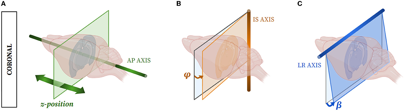
Figure 1. The three parameters used to exactly evaluate the 2D location of a coronal mouse brain slice within a template from an atlas: (A) the z-position along the AP axis, (B) the possible tilting angle φ around the IS axis, and (C) the possible tilting angle β around the LR axis.

Some studies focused on identifying possible tilting angles φ and β to refine 2D-plan location within the 3D atlas space (Xiong et al., 2018), while others proposed automated methods or user-friendly softwares to handle 2D slices within a 3D space toward z-position-oriented estimation (Puchades et al., 2019; Tappan et al., 2019). These strategies present a more or less accurate estimation of both tilting angles and are not fully automated since they all include manual processing to estimate the z-position. Basically, manual processing limits the use of such methods on a large scale for the study of mouse cohorts, in particular. More recently, a feature-based method called AMaSiNe was proposed to automatically estimate z-position, φ, and β (Song et al., 2020). Authors evaluate them with precision (<100 μm), and segmentation results have been validated on two specific small regions only (primary visual area and dorsal lateral geniculate complex). However, the method is non-reproducible for the analysis of a single slice. In addition, the method is only robust from a minimum of three slices. Finally, a completely different approach has been proposed, using deep neural networks (Sadeghi et al., 2022; Carey et al., 2023). These methods require a large number of slices to train the network and rely on manual ground truth definition. Such estimates are prone to inter- and intra-individual error; their result is subjective and usually performed only on a relatively small part of the dataset. Moreover, the large variety of histological staining, along with the different imaging modalities, makes it very difficult to build up an exhaustive database to train a fairly generic neural network. Most of the existing methods are either very complex and not user-friendly (codes without interface) to be implemented by neurobiologists or require knowledge in neuroanatomy to be used appropriately, both greatly reducing their scope of application.

The method we propose is intended to be generic enough to be used by anyone and benefits from a user-friendly interface. The fully automatic mode we propose gives reliable results, and the user can still adjust parameters. We focused on the estimation of the z-position of single coronal slices. Our automated method is reproducible and can align and segment any number of single slices within a digital 3D atlas. Moreover, we developed a dedicated multi-slices extension to meet ROI-driven histological protocols, resulting in a set of slices from the same brain. Our method is based on a linear registration algorithm as well as an independent and multimodal similarity criterion. The Block Matching (BM) algorithm (Ourselin et al., 2001) was chosen as a robust strategy to register data from different modalities. This method was later included in the NiftyReg library (Modat et al., 2014) and is still well used in many applications (Niedworok et al., 2016; Iglesias et al., 2018; Balakrishnan et al., 2019; Borovec et al., 2020; Mancini et al., 2020). Normalized Mutual Information (NMI) (Studholme et al., 1998) was chosen as a robust similarity metric adapted to multimodality. This metric has proven its efficiency in many biomedical image processing applications (Jefferis et al., 2007; Geha et al., 2008; Dorocic et al., 2014; Costa et al., 2016). The idea of the method is to explore registrations between the experimental single slice and the ones from the atlas template, with increasing degrees of freedom. The NMI criterion is used to propose a generic evaluation framework of the relative similarity between slices after each step of registration. Basically, the method combines similarity information coming from Rigid and Aff ine registration, which explains the acronym we defined for this method: giRAff. We chose to refer to the Allen mouse Brain Atlas (ABA), a digital atlas widely used in neurobiology (Lein et al., 2007; Lau et al., 2008; Kuan et al., 2015). Also, we focused on histological slices covering the cortex, excluding the main olfactory bulb and the cerebellum. Most of the biological samples come from healthy subjects, but we also present some preliminary results on a pathological subject (Alzheimer's disease mouse model).

In addition, high-performance computing strategies were used to reach our goal of segmenting a large number of histological slices. Indeed, as registrations have a relatively high computational cost, calculations were distributed on hundreds of CPU cores through the dedicated tool SomaWorkflow (Laguitton et al., 2011). Finally, to make the method easy-to-use, it was implemented within the user-friendly open-source software interface BrainVISA (Cointepas et al., 2001; Lebenberg et al., 2010).

2 Materials and methods

2.1 Materials

2.1.1 Digital mouse brain atlas

In this study, we used the template and atlas from the Allen mouse Brain Atlas (ABA) (© 2015 Allen Institute for Brain Science. Allen Brain Atlas API. Available from: brain-map.org/api/index.html). It is composed of two perfectly aligned datasets: a template that represents the average anatomy of the mouse brain and labels that represent the theoretical delimitation of anatomical regions delineated by an expert on the template data. This template was built as an average autofluorescence of 1,675 serial two-photon tomography C57Bl/6J mouse brains, for which we considered each coronal slice T_a ϵ B independently. B is the ensemble of slices describing the template volume considered a succession of independent slices in a given incidence (here coronal). The slice thickness is e_t = 100 μm and the in-plane resolution is 10 × 10 μm². In this study, we aimed to register 2D template images onto experimental histological slices. The purpose is to identify in the single slice of interest all the regions defined in the ABA reference corresponding slice.

2.1.2 Histological dataset

In this study, we aim to segment single 2D mouse brain coronal slices I_r, digitized from two different and independent histological modalities (see Supplementary material S0 for detailed protocols).

The first modality (so-called autofluorescence) is the autofluorescence of six clarified half mouse brains (M₁-M₆) imaged using light sheet fluorescence microscopy (Renier et al., 2016) that are considered as a succession of 2D coronal slices I_r devoid of cutting artifacts by nature. Those data were initially acquired with a resolution of 4 × 4 × 3 μm³ and resampled to 25 × 25 × 100 μm³ to generate a standard histological dataset.

The second modality (so-called cresyl violet) is cresyl violet-based Nissl staining of seven mouse whole brains produced in our laboratory (Vandenberghe et al., 2016) cut in the coronal incidence (I_r) using a microtome and digitized with a flatbed scanner. This second dataset includes six C57Bl/6J wild-type mouse brains (M₇-M₁₂) and one APP/PS1dE9 amyloid mouse brain (M₁₃), a transgenic mouse model of Alzheimer's disease (Dudeffant et al., 2017). The slice thickness is e_r = 20 μm (one every four slices) and the in-plane resolution is 25 × 25 μm². Regarding the cutting protocol, no specific instructions were given to prevent tilting angles. The cresyl violet data arose from our laboratory routine protocols in conventional histology.

2.2 Methods

2.2.1 Preprocessing

The template slices were first resampled in 2D to make the pixel size identical to the experimental data. Thus, the same number of pixels were used in the registration process by BM.

All images were resampled at 25 × 25 μm² for registration. This resampling was chosen as a compromise between a pixel size small enough to apply the registration in a reasonable time and large enough to preserve sufficient details in the image for the registration algorithm. In such a conventional histology study, data are commonly resampled at an in-plane resolution of 25 × 25 μm² (Renier et al., 2016) or 50 × 50 μm² (Song et al., 2020).

The template slices were also manually centered to correspond to the experimental images. This gave a good initialization, minimizing the amplitude of the displacements induced by the registration process and maximizing the tissue overlap at an equivalent field of view.

2.2.2 The giRAff method for one single slice

The giRAff method estimates the z-position of a single mouse brain slice within an atlas volume at a given incidence and considers zero or negligible tilting angles. This estimated z-position is associated with a transformation resulting from the registration between the corresponding template slice at the z-position and the experimental slice. The estimation of the z-position is given by the optimum of a similarity criterion estimated between the experimental slice considered and a set of registered slices from the template. The final result is the atlas segmentation of the single experimental slice considered through the registered and identified corresponding label slice.

The method is based on the atlas from the ABA and the linear registration method by Block Matching (BM) based on the Crossed Correlation (CC) similarity metric with the default parameters given by Ourselin et al. (2001), designed for such a histological dataset. Normalized Mutual Information (NMI) is the independent metric that quantifies the similarity between the registered template slices and the experimental single slice considered in pairs.

Given an incidence (here coronal), consider I_r an experimental single slice to be segmented by atlas and T_a a slice from an ensemble B of slices describing the template volume considered as a succession of independent slices, such as {T_a ϵ B}. Let L_a be a slice from an ensemble A of slices describing the labels considered as a succession of independent slices, such as {L_a ϵ A}, A and B being in the same geometry and perfectly aligned. Let N be the number of considered template slices in a given incidence (along the AP, IS, or LR axis), a ϵ ℕ^*, going from 1 to N, the considered template slice number. Each template slice (from B) has its corresponding slice containing the labels (from A). Assume z = â, the estimated position of the slice I_r within the template, i.e., the corresponding slice containing the labels. We chose to register template images (test) onto the experimental data (reference) to preserve the native geometry of the single slice (experimental) given as input by a user. Hence, labels will be mapped in the end onto the single slice to match its initial configuration.

The exploratory process for each image T_a ϵ B is carried out in three steps (Figure 2), with RIG and AFF representing the rigid and affine transformation space, respectively:

Figure 2

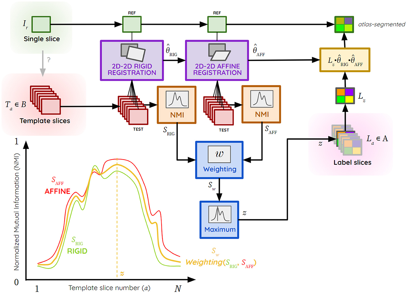
Figure 2. Atlas segmentation process of a single brain slice I_r by the giRAff method using template slices T_a ϵ B, theoretical example of NMI curve plots with S_RIG (green), S_AFF (red) and S_w (yellow), z the template slice number corresponding to a slice I_r estimated by the giRAff method, ${\widehat{\theta }}_{\text{RIG}}$ the rigid transformation, ${\widehat{\theta }}_{\text{AFF}}$ the affine transformation, B the ensemble of template slices, and L_a ϵ A the ensemble of label slices matching the template ones.

(1) Rigid registration using BM (transformation ${\widehat{\theta }}_{\text{RIG}}$) between I_r (reference) and T_a (test) from B, followed by an NMI similarity calculation S_RIG between the registered image $T_a·{\widehat{\theta }}_{\text{RIG}}$ and I_r,

$\begin{array}{ll}{S}_{\text{RIG}}(I_r,T_a;{\widehat{\theta }}_{\text{RIG}})=\text{NMI}(I_r,T_a○{\widehat{\theta }}_{\text{RIG}})& (1)\end{array}$

$\begin{array}{l}\text{ with }{\widehat{\theta }}_{\text{RIG}}={\displaystyle \underset{{\theta }_{\text{RIG}}\in \text{RIG}}{argmax}}(\text{CC}(I_r,T_a○{\theta }_{\text{RIG}}))\end{array}$

(2) Affine registration using BM (transformation ${\widehat{\theta }}_{\text{AFF}}$) between I_r (reference) and $T_a·{\widehat{\theta }}_{\text{RIG}}$ (test) registered in rigid (initialization), followed by NMI similarity calculation S_AFF between the registered image $T_a·{\widehat{\theta }}_{\text{RIG}}·{\widehat{\theta }}_{\text{AFF}}$ and I_r,

$\begin{array}{ll}{S}_{\text{AFF}}(I_r,T_a;{\widehat{\theta }}_{\text{AFF}})=\text{NMI}(I_r,T_a○{\widehat{\theta }}_{\text{RIG}}○{\widehat{\theta }}_{\text{AFF}})& (2)\end{array}$

$\begin{array}{l}with{\widehat{\theta }}_{\text{AFF}}={\displaystyle \underset{{\theta }_{\text{AFF}}\in \text{AFF}}{argmax}}(CC(I_r,T_a○{\theta }_{\text{RIG}}○{\theta }_{\text{AFF}}))\end{array}$

(3) Calculation of the weighted average S_w from the two similarity values S_RIG and S_AFF:

$\begin{array}{l}{S}_w(I_r,T_a,{\widehat{\theta }}_{\text{RIG}},{\widehat{\theta }}_{\text{AFF}})=(1-w)S_{\text{RIG}}(I_r,T_a;{\widehat{\theta }}_{\text{RIG}})\\ +w{S}_{\text{AFF}}(I_r,T_a;{\widehat{\theta }}_{\text{RIG}},{\widehat{\theta }}_{\text{AFF}})& (3)\end{array}$

with 0 ≤ w ≤ 1 the rigid-affine weighting.

From the weighted average S_w calculated for each slice T_a from B, a search of the maximum of similarity is performed to determine the slice number z from B, maximizing this similarity criterion from the N template slices:

$\begin{array}{ll}z(I_r,B)={\displaystyle \underset{T_a\in B}{argmax}}(S_w(I_r,T_a,{\widehat{\theta }}_{\text{RIG}},{\widehat{\theta }}_{\text{AFF}}))& (4)\end{array}$

Thus, the result of the giRAff method can be summarized as follows:

$\begin{array}{ll}\text{giRAff}(I_r,B)=(z,{\hat{\theta }}_{\text{RIG}},{\hat{\theta }}_{\text{AFF}})& (5)\end{array}$

The rigid and affine transformations ${\widehat{\theta }}_{\text{RIG}}$ and ${\widehat{\theta }}_{\text{AFF}}$ estimated by BM are successively applied at the slice L_â from the atlas at the position â = z to superimpose the registered image containing the labels ${\widehat{L}}_{â}$ on I_r, the experimental image.

$\begin{array}{ll}{\hat{L}}_{â}(z,{\hat{\theta }}_{\text{RIG}},{\hat{\theta }}_{\text{AFF}})=L_z○{\hat{\theta }}_{\text{RIG}}○{\hat{\theta }}_{\text{AFF}}& (6)\end{array}$

The transformation matrices ${\widehat{\theta }}_{\text{RIG}}$ and ${\widehat{\theta }}_{\text{AFF}}$ are applied to the slice L_â with the nearest neighbor interpolation to preserve the initial values of the labels. The experimental single slice I_r is then automatically segmented by the ABA. Quantitative region-based analysis can then be carried out on it thanks to the method.

2.2.3 The giRAff_m extension for a multi-slices case

2.2.3.1 Relative scaling factor between brain samples

Two mouse brains are often considered to be roughly the same size, but this is not the case in practice. Two factors influence the size of the organ, in particular: inter-individual variability (natural) and the extraction, cutting, and staining protocol to which the sample is subjected before analysis (non-natural).

Let us consider a multi-slices case, i.e., a series of single histological slices from the same mouse brain not enabling its 3D reconstruction. Let d_r be the constant inter-slice distance between single slices from the experimental volume. Let d_t be the inter-slice distance between slices from the template volume. To realistically estimate the corresponding distance d_r depending on d_t in the template, the differences in brain volumetrics must be taken into account. Not taking them into account would lead to a deviation in the estimation of successive slice positions (Figure 3A). For this reason, a relative scaling factor γ (RSF) was introduced, which reflects the size difference between an experimental brain and the atlas template volume on the axis to which the considered incidence plane is orthogonal (Figure 3B). The affine registration automatically corrects the scaling factors in the other two directions (α, β) relative to the plane of incidence considered. This RSF γ is relative because no modality accounts for an absolute reference geometry: it is relative between two modalities.

Figure 3

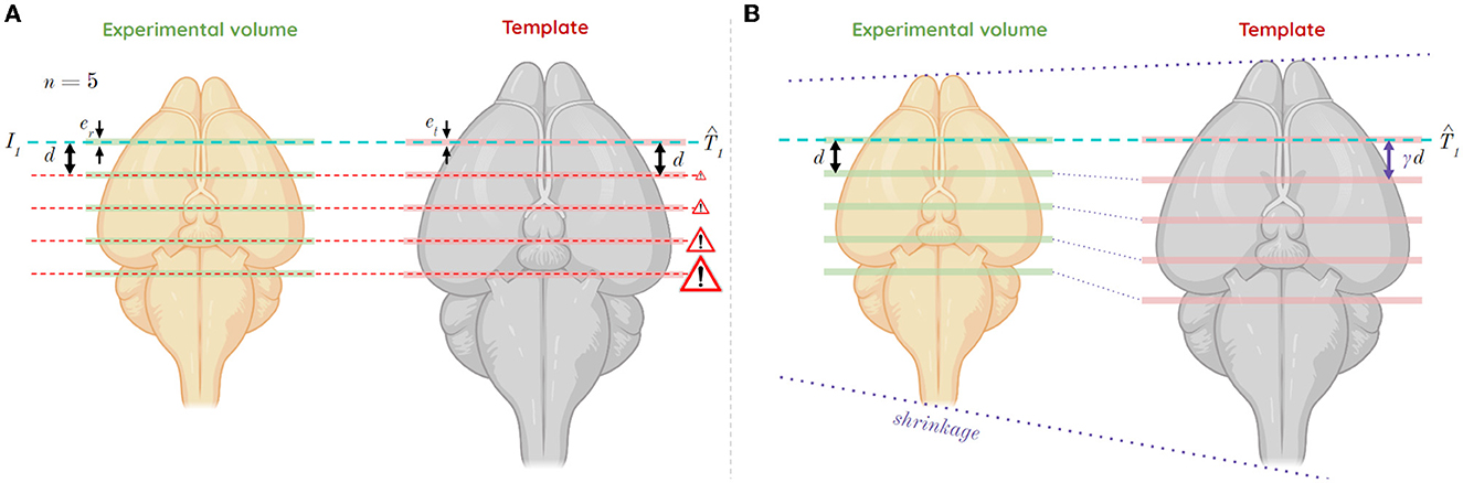
Figure 3. Shrinkage case of the experimental volume compared to the template volume, and its impact in a multi-slices study in the coronal incidence along the AP axis, for slice thicknesses e_r and e_t from the experimental and template volumes, respectively, as well as an inter-slice distance d between each considered slice from the experimental volume. (A) Study of five slices from a first T₁ estimate without consideration of shrinkage between volumes (mismatch). (B) Study of five slices from a first estimate T₁ considering the shrinkage between volumes using RSF γ (correction).

Thus, assume:

$\begin{array}{l}\{\begin{array}{lll}0<\gamma <1& \iff & \text{shrinkage}\\ \gamma =1& \iff & \text{same size}\\ 1<\gamma <+\infty & \iff & \text{enlargment}\end{array}\end{array}$

The distances d_r and d_t are defined as a function of γ and the two slice thicknesses e_r for the experimental data and e_t for the template data:

$\begin{array}{ll}{d}_r=\gamma \frac{e_r}{e_t}{d}_t& (7)\end{array}$

Let r ϵ N^* be the slice number from the experimental data ranging from r = 1 to r = M, and t the slice number estimated to be the most similar in the template by the giRAff method, ranging from t = 1 to t = N. The equation of the affine line linking slice numbers from the two volumes to each other can thus be deduced:

$\begin{array}{ll}\widehat{t}(r)=\gamma \frac{e_t}{e_r}(r-1)+{\widehat{t}}_1& (8)\end{array}$

with $\widehat{t_1}$ the y-intercept corresponding to the result of the giRAff method applied to the first slice of the experimental volume studied (r = 1).

2.2.3.2 Operating mode

For each considered experimental single slice from a multi-slices set, similarity values with all the template slices are computed by the giRAff method and stored in a list s_w (see Equation 3, which is applied for each slice T_a ϵ B). The multi-slices analysis aims to bring each of these lists into a single referential to pool their contribution.

Assume (u_s${)}_{sϵ{\text{N}}^{*}}$ an arithmetic series determining the first template slice number to be tested in the case of a multi-slices study and (v_s${)}_{sϵ{\text{N}}^{*}}$ an arithmetic series determining the last template slice number to be tested in the case of a multi-slices study, we then have:

$\begin{array}{l}{u}_s=u_1+\frac{d_t}{e_t}(s-1)and{v}_s=N-\frac{d_t}{e_t}(n-s)(9)and(10)\end{array}$

with u₁ = 1 corresponding to the first template slice number.

Values from the series (u_s${)}_{sϵ{\text{N}}^{*}}$ and (v_s${)}_{sϵ{\text{N}}^{*}}$ are rounded to the nearest integer so that they correspond to real slice numbers.

The giRAff method is successively executed for each slice s, solely on a range of template slices B_[us;vs] ⊂ B defined by the two series. This range contains the same number of slices d_t/e_t rounded off to the nearest unit. This amounts to determining the z-position of the first studied slice from the mutualization of the similarity information S_w of all the slices in the multi-slices set. Once this z-position has been estimated in a common manner, it is propagated to the other slices of the series to determine their respective z-positions. The position of the other slices is deducted by adding the distance d_t in the template corresponding to the distance d_r, which separates the slices from each other in the experimental volume. Assuming z_m is the z-position estimated by combining different similarity information in the multi-slices case, as with the classical giRAff method, a calculation of the maximum similarity is then performed to determine the desired position z_m:

$\begin{array}{ll}{z}_m(E,B)={\displaystyle \underset{T_a\in B_{\left[u_s;v_s\right]}}{argmax}}\left(\frac{1}{n}{\displaystyle \sum _{s=1}^n}{\pi }_s{S}_w(I_s,B_{\left[u_s;v_s\right]},{\widehat{\theta }{}_{\text{RIG}}}_s,{\widehat{\theta }{}_{\text{AFF}}}_s)\right)& (11)\end{array}$

with S_w being a list containing the averaged NMI values for rigid and affine registration (see Equation 3), E a multi-slices ensemble, and π_s the contribution rate for each slice s (π_s = 1/n by default, giving an equal contribution for each slice).

Assume giRAff_m is the extension of the giRAff method to a multi-slices study, which is defined as:

$\begin{array}{ll}\text{g}iRAf{f}_m(E,B)=(z_s,{\hat{\theta }{}_{\text{RIG}}}_s,{\hat{\theta }{}_{\text{AFF}}}_s)& (12)\end{array}$

For each slice I_s from E, a z_s position (deduced from z_m) as well as rigid and affine transformations ${\widehat{\theta }}_{\text{RIGs}}$ and ${\widehat{\theta }}_{\text{AFFs}}$ are determined, which allows the identified label slice L_â to be mapped onto the experimental single slice I_s. The contribution of each slice I_s can be adjusted toward the weight π_s. For example, if a slice I_s has many artifacts that might compromise the registration with the template slices, it is possible to manually adjust its influence by decreasing its contribution π_s or even remove it from the z_m estimation (π_s = 0).

The numbers z_s = t_s of each of the slices from the multi-slices study from E can directly be calculated from z_m:

$\begin{array}{ll}{z}_s=z_m+s{d}_t=\widehat{t_1}+s\frac{e_t}{\gamma e_r}{d}_r& (13)\end{array}$

with $\widehat{t_s}$ rounded to correspond to real slice numbers (integers). An affine transformation ${\widehat{\theta }}_{\text{AFF}s}$ is associated with each position z_s.

2.2.4 giRAffMapper: a generic pipeline

The generic pipeline giRAffMapper automatically performs the atlas segmentation of any number of slices corresponding to any histological experimental protocol. Let S^* be the needed and required number of slices to reconstruct a 3D brain. Whether it is for the analysis of a single slice (n = 1), for several slices in the analysis of a particular anatomical region (1 < n < S^*), or for a large enough number of slices to perform a 3D reconstruction of the brain (n ≥ S^*), the giRAffMapper generic pipeline automatically processes any histological brain slice protocols (Figure 4).

Figure 4

Figure 4. giRAffMapper generic pipeline performing the automated atlas segmentation of any number n of histological slices using the giRAff method as well as its extension giRAff_m. S* represents the needed and required number of slices to reconstruct a 3D brain.

2.2.5 Validation of the method

2.2.5.1 Metrics of validation

As our aim is to achieve an atlas segmentation as accurate as that of experts, we took the quantitative results of a neuroanatomist's evaluation as a reference. We asked an expert to identify the right number (z-position) of the template slice being the most similar to each experimental considered slice I_r, the so-called Expert Rating for the z-position (ER_z) (see Supplementary material S1). This made it possible to define the deviation of the z-position Δ_sn between ER_z and the z-position estimated by giRAff:

$\begin{array}{ll}{\Delta }_{sn}(I_r,B)=|E{R}_z(I_r,B)-z(I_r,B)|& (14)\end{array}$

The final purpose being the segmentation of anatomical regions, we also calculated dice scores (Dice, 1945) between the manual segmentation from an expert on the experimental considered slice and the one resulting from the identified and registered template slice by the giRAff method. We then compared these obtained dice scores to those calculated after prior identification of the z-position by an expert.

2.2.5.2 Realistic histological protocols to perform region-based analysis

We designed realistic region-based histological protocols from mouse whole brain histological datasets with an expert. Six main regions of interest were chosen from different sizes and locations in the brain: cortex, striatum, hippocampus, thalamus, globus pallidus, and substantia nigra. We especially selected them because of their known involvement in neurodegeneration, especially concerning Alzheimer's, Parkinson's, or Huntington's diseases (Dostrovsky et al., 2002; Picconi et al., 2005; Teichmann et al., 2005). For each anatomical region, the protocol includes the identification of the respective slices in which this region starts and ends along the AP axis, as well as the number of slices to be considered and their inter-slice distance, allowing quantitative studies (see Supplementary material S2). To assess the robustness of such an exploratory approach, we tested all possible protocol combinations covering each region and brain considered, given a constant inter-slice distance.

2.2.6 Determination of the rigid-affine weighting w for a given imaging modality

To determine the optimal rigid-affine weighting to be applied for a given imaging modality, we evaluated the average Δ_sn values for each possible weighting, using steps of 0.01, for all the slices from the brains in a given modality. From this evaluation, we estimated an average curve of Δ_sn as a function of w, which gave us an average trend displaying which rigid-affine weighting w minimizes deviation Δ_sn and, therefore, maximizes the accuracy of the method. To get a realistic idea of this trend for conventional histological slices, it is necessary to exclude from the overall estimate brains suffering from too many artifacts (air bubbles, tearing, missing tissue, etc.) that could compromise this evaluation.

2.3 Implementation details and source code

Considering the large number of calculations, the pipeline was run using distributed computing on multiple microprocessors using the SomaWorkflow library of BrainVISA software (Laguitton et al., 2011). BrainVISA is an open-source software platform for neuroimaging research, including visualization tools and graphical user interfaces (https://brainvisa.info). This study was conducted on a workstation Ubuntu 16.04; LTS 64-bits; Intel^® Xeon^® CPU E5-2620 v2 @ 2.10GHz × 24 (24 computing cores); 128 GB of Random Access Memory (RAM), with the support of our Titan2 calculator composed of five DELL R610 bi-processor nodes on Intel^® Xeon^® CPU X5675 @ 3.07GHz × 12 and 48 Go of RAM, one DELL R610 bi-processor node on Intel^® Xeon^® CPU X5667 @ 3.07GHz × 8 and 48 Go of RAM, and six DELL R630 bi-processor nodes on Intel^® Xeon^® CPU E5-2630 v3 @ 2.40GHz × 16 and 128 Go of RAM (representing 328 computing cores overall).

3 Results

The giRAff method has the advantage of being exhaustive in exploring all the possible correspondences after linear registration between a single slice under study and the slices from the average template. This exploration is performed in a minimum of time thanks to a distributed implementation. The choice of the registration algorithm as well as the similarity metric was made to suit multimodal studies, and their independence provides robustness in the identification of the right z-position for a given single slice.

The giRAff_m extension has been specially designed for multi-slices studies, where the RSF is taken into account for an accurate and realistic estimation of the common z-position for a given dataset.

All these developments are gathered in a generic pipeline able to automatically segment any number of slices by atlas. The method presents the advantage of being embedded in an easy-to-use software for simple utilization (see Supplementary material S6).

We used two complementary metrics to evaluate the efficiency of the method in its two different aims: its ability to identify the right z-position of single histological slices, whatever their number, and its ability to present relatively good atlas segmentation scores after registration.

3.1 Single histological slice segmentation by giRAff

3.1.1 Determination of the rigid-affine weighting w

We first evaluated which rigid-affine weight w minimizes the Δ_sn criterion for each modality: the autofluorescence (Figure 5A) and the cresyl violet (Figure 6A). For the autofluorescence, the trend was clearly not toward a rigid-affine weighting w at extremes (0 or 1). No particular weighting appeared to be especially optimal between these extreme values. We therefore chose a rigid-affine weighting w = 0.50 for this modality to ensure robustness in the use of the two types of registration and to avoid the extreme weightings, which can be a source of misidentification (high Δ_sn). Concerning cresyl violet, it was necessary to remove data presenting too important artifacts (M₇), making them non-representative for the evaluation of the global trend of the rigid-affine weighting w. In contrast to autofluorescence modality, a clear trend appeared in favor of a weighting w = 1 for the cresyl violet, which minimized mean Δ_sn. This means that the NMI resulting from affine registration prevailed for this imaging modality in the estimation of the z-position of single slices in comparison to an expert.

Figure 5

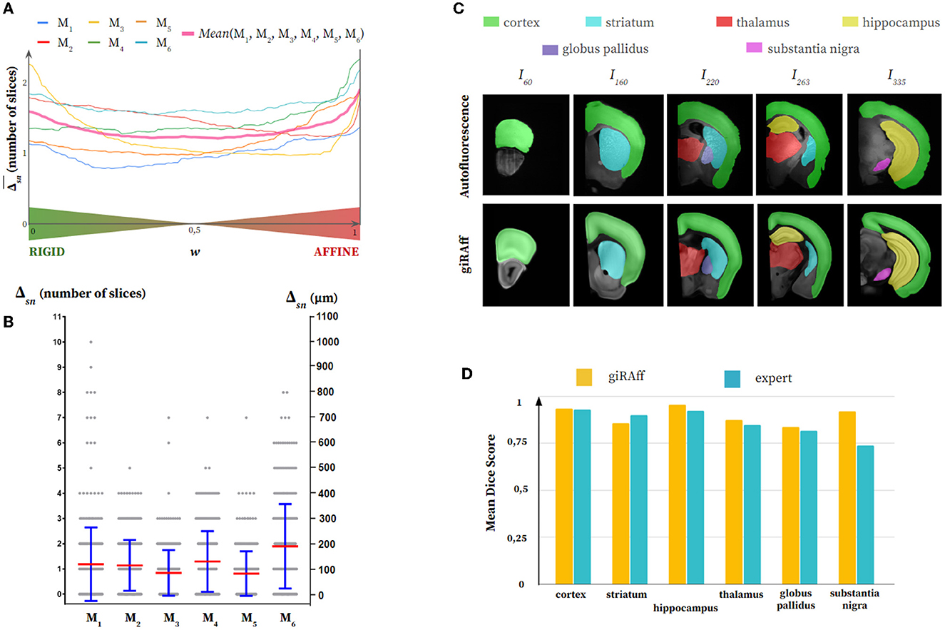
Figure 5. Single slice manual segmentation of the Autofluorescence half mouse brains (M₁-M₆): (A) Averaged Δ_sn values after application of the giRAff method for each rigid-affine weighting w from 0 to 1 by 1% increments, (B) Δ_sn values (gray) after application of the giRAff method (mean in red and standard deviation in blue) for each single slice, (C) segmentation of six anatomical regions of interest of various sizes (cortex, striatum, hippocampus, thalamus, globus pallidus, and substantia nigra) by an expert in five experimental single slices across the brain M₁ (first row) as well as their corresponding registered template slice identified by the giRAff method (second row), and (D) non-weighted mean dice scores (see Supplementary material S4) evaluated on the six anatomical regions for the five slices identified and registered from (C) between the giRAff method (yellow) and an expert (cyan).

Figure 6

Figure 6. Single slice manual segmentation of the seven cresyl violet mouse brains (M₇-M₁₃): (A) Averaged Δ_sn values after application of the giRAff method for each rigid-affine weighting w from 0 to 1 by 1% increments, (B) Δ_sn values (gray) after application of the giRAff method (mean in red and standard deviation in blue) for each single slice, (C) segmentation of six anatomical regions of interest of various sizes (cortex, striatum, hippocampus, thalamus, globus pallidus, and substantia nigra) by an expert in five experimental single slices across the brain M₁₀ as well as their corresponding registered template slice identified by the giRAff method, and (D) non-weighted mean dice scores (see Supplementary material S4) evaluated on the six anatomical regions for the five slices from (C) between the giRAff method (yellow) and an expert (cyan).

3.1.2 Precision and robustness of the method

The giRAff method was applied independently on 2,135 single half-slices (one hemisphere) and 636 whole slices (whole brain) from two modalities from 13 mouse brains. In routine protocols performed in our laboratory, φ and β angles were estimated below 5° (see Supplementary material S3) and were neglected in this study. The deviation Δ_sn compared to an expert was calculated for every single slice considered from this dataset. The giRAff method was able to identify any single mouse brain slice with an average accuracy of 1.20 ± 1.19 and 2.05 ± 3.05 slices for the autofluorescence and the cresyl violet, respectively (Table 1). This represented an average precision of the z-position identification between 120 and 164 μm, respectively.

Table 1

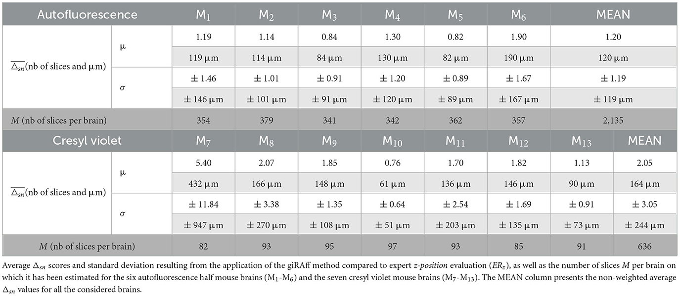
Table 1. Single slices—autofluorescence and cresyl violet.

Concerning the autofluorescence, no high Δ_sn scores appeared, being mainly narrow around 0 and 200 μm, the largest deviation of 10 slices being obtained only once (M₁) among the six brains (Figure 5B). If we look qualitatively at the segmentation of the anatomical regions of interest, we notice that their delineation is close to that performed by an expert on the experimental slice (Figure 5C). From the smallest of the regions studied (substantia nigra) to the most elongated (cortex), the segmented shapes were quite close. These results were confirmed quantitatively by the dice scores (Figure 5D; see Supplementary material S4) evaluated on five slices among the brain M₁, which demonstrated the capacity of the giRAff method to obtain fairly high scores (around 0.90) after identification of the z-position for a given experimental slice. More importantly, those dice scores were widely comparable to those of an expert.

Results for cresyl violet appeared to be somewhat less accurate, with Δ_sn scores being concentrated more between 0 and 300 μm on average, with the exception of M₇, for which values were significantly higher (Figure 6B). Misidentifications above 10 slices of deviation were also rare. The qualitative analysis of the segmentations showed that the anatomical regions corresponded rather well, with some small differences, in proportion for the substantia nigra or in shape for the striatum (Figure 6C). These small differences had very little impact on the dice score, which remained globally quite high (around 0.85), except for the substantia nigra and the globus pallidus (around 0.75). Similarly and most importantly, dice scores showed that segmentation results using the giRAff method on these five slices were still widely comparable to those of an expert (Figure 6D; see Supplementary material S4).

All in all, no particular difference in the accuracy of the giRAff method was noticed in identifying the z-position of slices from a brain including pathological lesions (M₁₃) compared to other brains (M₇-M₁₂): average Δ_sn and standard deviation (1.13 ± 0.91 slices) of M₁₃ were significantly inferior to the mean evaluation on the whole cresyl violet dataset (2.05 ± 3.05 slices).

3.2 Multi-slices histological segmentation by giRAff_m

Based on the rigid-affine weighting empirically determined for each of the two modalities, the giRAff_m extension was applied on multi-slices datasets based on routine histological sectioning protocols. Those protocols were designed by experts to correspond to studies of particular anatomical regions of different sizes in the coronal incidence: cortex, striatum, thalamus, hippocampus, globus pallidus, and substantia nigra (see Supplementary material S2). These conventional protocols involved a number of slices and an inter-slice distance, with the first slice of a given region being shifted at each iteration so that the entirety of the slices constituting each region were tested. The deviation Δ_sn was calculated for each slice included in every multi-slices case, and the result was averaged per anatomical region studied.

The deviation Δ_sn was estimated in three different contexts: (1) using the giRAff method considering each slice as single (same case as in Section 3.1 focused on the slices including each anatomical region considered), (2) using the giRAff_m extension considering multi-slices protocols and an RSF γ_Mi evaluated for each brain thanks to the ER_z, and (3) using the giRAff_m extension considering multi-slices protocols and an averaged RSF γ_m evaluated for a given protocol and imaging modality (see Supplementary material S5).

Concerning the autofluorescence, first, the multi-slices approach significantly reduced the average deviation Δ_sn and its dispersion, in general: Δ_sn criterion underwent a reduction between 55 and 105 μm and the standard deviation between 53 and 87% depending on the region, on average (Table 2; Figure 7A). The case of considering the RSF γ_Mi specific to each volume M_i (i ranging from 1 to 6) presented smaller deviations Δ_sn than the case of an average RSF γ_m (increase of the order of 8%). Depending on the experimental conditions that were applied to each volume, considering γ_Mi specific to each of them made it possible to obtain better accuracy in the detection of the z_m position. Estimating an accurate value of this RSF γ increased the precision of detecting the right position z_m by the giRAff_m extension. On average, over all regions, the accuracy of z_m position detection in the multi-slices case by the giRAff_m extension was equal to 57 ± 49 μm with γ_Mi and 63 ± 52 μm with γ_m for the autofluorescence.

Table 2

Table 2. Multi-slices—autofluorescence and cresyl violet.

Figure 7

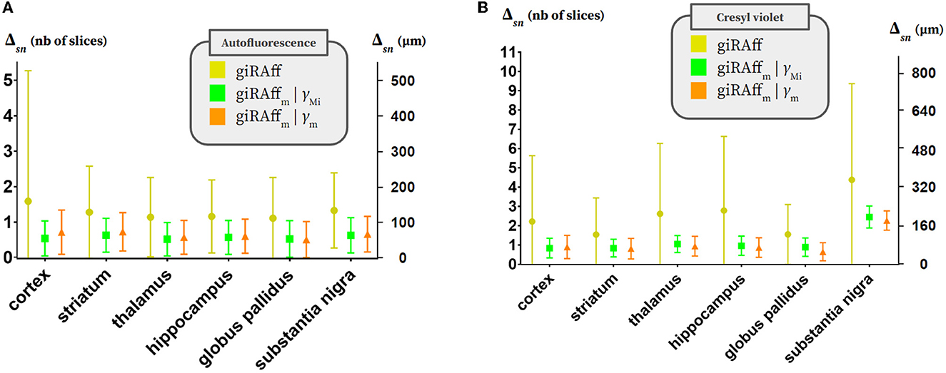
Figure 7. Multi-slices. Averaged Δ_sn values and standard deviation per considered anatomical region (cortex, striatum, hippocampus, thalamus, globus pallidus, and substantia nigra) in three different contexts: using the giRAff method considering each slice as single (yellow), using the giRAff_m extension considering multi-slices and RSF γ_Mi evaluated for each brain thanks to the ER_z (green), and using the giRAff_m extension considering multi-slices and an averaged RSF γ_m evaluated for a given protocol and imaging modality (orange) for (A) the six autofluorescence brains and (B) the seven cresyl violet brains.

Regarding the cresyl violet, second, the multi-slices approach strongly decreased the average deviation Δ_sn and its dispersion in general: Δ_sn criterion underwent a reduction between 53 and 169 μm, and the standard deviation between 69 and 90% depending on the region, on average (Table 2; Figure 7B). The use of the giRAff_m extension in the multi-slices case significantly improved the overall detection accuracy of the z_m position in this modality. In contrast to what was observed for the autofluorescence data, the γ_m case presented better results (Δ_sn decreased by 4% on average over all regions) than for the consideration of the respective γ_Mi. Only the cortex region showed Δ_sn(γ_Mi) > Δ_sn(γ_m) by 7%. For the other regions, considering γ_m rather than γ_Mi improved the detection of the correct z-position by 4% (striatum) to 27% (globus pallidus). On average, over all regions, the accuracy of z_m position detection in the multi-slices case by the giRAff_m method was 94 ± 54 μm with γ_m. Whatever the case considered, the substantia nigra was the only region with high deviations: the accuracy Δ_sn was 180 ± 40 μm while it was always <80 μm for all other regions. Atlas segmentation of small anatomical regions was more challenging than for large regions, both for experts and for the proposed method.

A gain in accuracy was clearly observed when using the giRAff_m extension compared to the giRAff method for the same slices considered independently: with a few exceptions, Δ_sn was brought down between 0 and 100 μm on average, whatever the modality and the region.

For one single slice, the giRAff method proposed an automated atlas segmentation in about 1 min using Titan2 infrastructure.

3.3 Cross-talk between giRAff and giRAff_m

Several single slices from cresyl violet mouse brains (M₇-M₁₃) suffered from histological artifacts. In most cases, the presence of a considerable artifact prevents segmentation of the entire histological slice. Such a slice is often discarded, or its segmentation is carried out manually if the damaged part does not concern the tissue of interest. Despite some considerable artifacts, the giRAff_m extension still allows for identification of the correct z-position and segment the rest of the slice correctly. Some examples including such artifacts (tissue folding, missing tissue, and external noise) are presented in Figure 8.

Figure 8

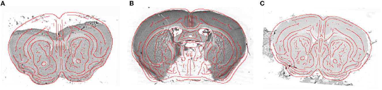
Figure 8. Example of histological single slices (cresyl violet) presenting histological artifacts: (A) tissue folding (M₁₁), (B) missing tissue (M₈), and (C) external noise (M₇), with the superposition of the red boundaries of the template slice, obtained using a Deriche filter (Deriche, 1990), at the z-position identified by the giRAff_m extension.

4 Discussion

In this study, we proposed a method to automatically segment one or a set of single slices using a 3D digital atlas. The giRAff method, based on linear registration tools and on the NMI as a similarity metric, showed its ability to deal with any number of slices, adapting to very different standard histological protocols (3D fluorescence and 2D brightfield imaging). We demonstrated the robustness and the efficiency of the method by applying it on two different datasets: autofluorescence data, which was not affected by cutting artifacts, and histological slices from routine experimental protocols. It was indeed able to identify, depending on the protocol considered, the z-position of one or more single slice(s) with an accuracy of the order of one slice within the atlas template. This amounted to an identification deviation of less than about 100 μm on average, with dice scores comparable to those obtained by an expert. The method also showed its ability to deal with slices suffering from histological artifacts using the multi-slices approach.

The method was based on a balanced use of the similarity information evaluated after rigid and affine registration in an exploratory approach. In this context, the rigid-affine weighting w was of crucial importance as it allowed to adjust the use of NMI information to take advantage of the benefits from each type of registration. Indeed, in the exploratory approach we proposed, the two types of registration can be complementary. Rigid registration is often rough and avoids the identification of a particular slice that is the closest to the single slice considered, whereas affine registration makes the difference in improving tissue registration thanks to a greater number of degrees of freedom (shearing and scaling). On the contrary, affine registration could make slices correspond to each other with an inappropriate superposition of tissues forced by large deformations, whereas rigid registration does not allow such modifications, limits the deformations, and permits the differentiation of these slices. The use of a weighted proportion of the similarity information created a robust study framework for their comparison in an exploratory context. This represents a useful parameter to tune according to the amplitudes of the deformations considered or according to the biological protocol used. For the two modalities tested in this study, the trend was toward either 0.5 or 1. What we would suggest for users is to consider one or the other of the rigid-affine weighting given in the manuscript by default for their own data according to the imaging modality chosen. In the case of another specific imaging modality or for any doubt on the rigid-affine weighing chosen, the operator could easily test adjusting it from 0.5 to 1 or from 1 to 0.5. If this improves the result in their opinion for their own dataset, they should obviously reuse it by default for the next iterations with other data produced in the same modality. Initialization of the registration by centering the slices on each other was therefore a mandatory step in this gradual pipeline. Even if this centering process was presented as being manually performed in this study, it would be possible to readily add a simple algorithm to perform this task in an automated manner. Maximizing the overlap of the binarized tissue surface could be used, for example, to improve the method in the future.

The giRAff method was inspired by the operating mode an expert uses when manually identifying the position of a single slice: neuroanatomists flip atlas pages and try to match the shapes of certain anatomical regions in an exploratory way, as well as qualitatively estimate the similarity in a visual manner. Our pipeline does the same using linear registration and NMI. Although NMI has shown its robustness in various multimodal brain applications, its efficiency remains discussed within the scientific community (Zheng, 2006; Xiong et al., 2018; Song et al., 2020). This similarity metric is known to have non-significative values in absolute: comparing two objects whose nature does not have anything in common can even result in a significantly high NMI score (Rohlfing, 2011). The use of NMI was solely relative in our pipeline, considering its score on any template slice in comparison to each other. This information was never used in an absolute manner, and the nature of the objects being compared was the same, thus avoiding this limitation. The NMI was not used as a similarity metric to estimate registration but only to objectively evaluate the quality of the slice-to-slice correspondence after registration.

In the dataset we used, we purposely selected uncut 3D coherent histological brain volumes (autofluorescence of a cleared brain acquired with a light-sheet microscope), which was considered as a succession of 2D virtual slices. In such a way, it was possible to test different data processing approaches with artifact-free tissue. This could be one of the reasons why the precision of the z-position detection was better for the autofluorescence (lower Δ_sn) than for the cresyl violet. We first opted for this favorable context to make a proof of concept, taking autofluorescence as a kind of ideal case (Piluso et al., 2021a). Then, we confronted with “real life” histological preclinical routine protocols (digitized Nissl/cresyl violet-stained brain sections), based on our robust and adjustable pipeline.

When using the giRAff method for a given individual slice, its z-position is estimated only once. This estimate may suffer from deviations that could be due to the presence of artifacts in the slices, by poor quality registration, or by a relative similarity value that is not significant enough. In the giRAff_m approach, the joint estimation of the position z_m from a set of slices provided a statistical quantity of estimates sufficient to significantly reduce the deviation Δ_sn and its dispersion in general. This improvement was based on the assumption that a large majority of the slices had little or no artifact, and that the registration and similarity metric were robust enough to accurately estimate the z-position of such slices in the dataset. As a result, for one or several slice(s) suffering from artifacts, representing a minor proportion of a given dataset, giRAff_m provided better z-position identification results than giRAff.

On average, for a multi-slices dataset, the z-position of single slices was detected with a precision of one slice in the atlas (~ 100 μm). This deviation is comparable to the one that experts could make on such a dataset, as long as one single slice considered does not perfectly match one given slice in the template. Indeed, because of its slice thickness and its exact location on the AP axis, as well as possible tilting angles, experts sometimes hesitate between two adjacent slices from the template to identify the right z-position of an experimental single slice. Therefore, they are constrained to make an arbitrary choice, assuming that the position they have identified is only accurate within one slice (100 μm).

Some regions with little pixel support, such as substantia nigra, presented poor dice score results compared to other bigger regions with larger pixel supports. In the linear registration algorithm used, few degrees of liberty were allowed to try to optimize a global transformation at a whole-image scale. This obviously tended to maximize the overlap between regions, including larger pixel support at the expense of other smaller regions including significantly fewer voxels. In such regions, a difference of one single voxel was far more significant than in other regions. Using non-linear registration after estimating the z-position could significantly increase the overlap between such small regions and then significantly increase their dice score.

Concerning the cresyl violet data, the M₇ brain showed higher Δ_sn scores (larger deviation) than the other brains without using the multi-slices extension giRAff_m, confirmed by the presence of artifacts due to the histological and digitization protocols (bubbles, added tissue fragments, and external noise). This is a typical example of artifacts that can occur during a conventional histological protocol. Automatically segmenting histological slices with significant artifacts has always been a challenging task for the scientific community (Agarwal et al., 2016). Most of the time, automatic atlas segmentation of these slices is basically impossible. Our proposed giRAff_m extension has the advantage of optimizing z-position detection on a set E of multiple single slices, and thus could be able to identify and segment such slices including artifacts. Results were pooled to obtain the best z_m position estimated for all the slices. Thus, for a set of slices from the same brain, including slices with important artifacts, it was then possible to decrease their rate of contribution π_s (until 0) in the global estimation of the z_m position, but yet achieve their automatic segmentation reliably. Considering a majority of good quality slices selected from E and a robust regression (significantly high coefficient of determination, typically above 0.97), the giRAff_m extension can propose an automated atlas segmentation corresponding for any other slice suffering from those artifacts from the same brain in a robust way, especially without taking them into account in the global estimation of the position z_m. If the rate of contribution π_s was presented as a subjective parameter to add manually as input information within the multi-slices pipeline, further improvements could lead to the use of image processing algorithms able to automatically detect artifacts within histological slices (Agarwal et al., 2016). This would lead to an automated setup of the rate of contribution π_s for each single slice as a consequence. Moreover, using the multi-slices giRAff_m extension allowed for automated estimation of the RSF γ between the data considered. This reinforced the fact the method we proposed is versatile, robust, and adaptable to many types of protocols or histological brain data.

Considering a multi-slices dataset, we focused on a constant inter-slice distance between single slices under study in this article. But in practice, this distance could be heterogeneous. The principle of the multi-slices extension giRAff_m for the analysis of such slices would be exactly the same; the different inter-slice distances can be given as input information within the giRAff_m pipeline.

In conventional histological protocols, tilting angles may occur when slicing the 3D organ. A non-zero φ angle around the IS axis can generate anatomical differences between the left and right side of the slice, which are easy for an expert to identify due to the brain symmetry with respect to the interhemispheric plane. However, it is more challenging to identify a non-zero β angle around the LR axis that will generate differences between the top and bottom of the slice. This angle is most often observed as non-zero, and neurobiologists then have to deal with neighboring slices to perform the segmentation manually. Thanks to a rigid 3D-3D registration between each considered brain and the template volume, it was possible to estimate these tilting angles around the IS and LR axis, and they are of low amplitude (<5°, see Supplementary material S3), hence our focus on the z-position determination. Considering those realistic tilting angles of low amplitude, the accuracy of the giRAff method nevertheless made it possible to preserve automatic segmentations for which dice scores are still comparable to those of an expert. Indeed, as protocols for acquiring those brains may be representative of standard protocols in conventional brain histology performed in the coronal incidence, we assume that tilting angles rarely exceed an amplitude of 5° with modern equipment and in a similar study framework. If this angulation generates genuine anatomical differences compared to data without angulation, the method we proposed made it possible to compensate for this drawback. Indeed, we chose to process data produced in routine histological protocols in this article, i.e., including real tilting angles caused by the cutting process. Histological data presented in this article included their native tilting angles. As the giRAff method detected the z-position of the single slice with high accuracy, its anatomical environment was well identified (basically in the thickness range of about 200 μm). Following this location, registration ensured the best matching of the tissue between the single slice considered and the template slice identified, as it would have been done in the case of considering the respective adjacent slices of its direct neighborhood. In the coronal incidence and with a slice thickness of about a hundred micrometers, anatomical variations are small from one slice to the next adjacent one. The template data are smooth, and very few discontinuities appear when examining the slices one after the other along the AP axis. More specifically, a tilting angle would generate small anatomical differences between the right and left of the slice for an angle φ around the IS axis and between the top and bottom of the slice for an angle β around the LR axis compared to the template data. In practice, using linear registration would basically correct most of those segmentation errors because the presence and location of anatomical regions are almost the same from one slice n to its n-1 and n+1 (or more) neighbors. Indeed, anatomical differences generated by a tilting angle cause linear deformations along one, two, or both axes (IS and LR in the coronal incidence), which affine registration can compensate with shearing. This was confirmed by dice scores calculated, which were widely comparable to those of an expert in the end. The only necessary condition is that the z-position of the single slice considered must be accurately estimated, typically with a deviation less or equal to one slice in the template, to avoid too large anatomical difference between slices considered. It is just a matter of comparing data which are comparable, i.e., extracted, cut, and digitized within a rigorous, consistent, and realistic study framework. If neurobiologists are asked to cut coronal mouse brain slices using a microtome, it is reasonable to believe that their skills will enable them to obtain tilting angles below 5° as observed in the data presented in this article. Visual quality control and steel matrices could also be used for this purpose.

The method we proposed was based on linear registration in a pipeline with an increasing number of degrees of freedom. The use of non-linear registration could compromise the identification of the correct z-position of a given single slice. Indeed, too many degrees of freedom would excessively distort all template slices to match, in an inappropriate way, the single slice under consideration. It would then be challenging to distinguish which was the most similar. In contrast, the use of non-linear 2D-2D registration between the single slice and the template slice identified at the z-position at the end of the giRAff pipeline would certainly enable the segmentation results to be refined. This could be useful for the analysis of small regions, for example. This constitutes one of the further improvements the method could benefit from. Moreover, the lack of ground truth will make the task even harder.

A benchmark between the different methods of segmenting single slices should be carried out to identify which could give the best results according to the experimental data under study. Such a benchmark should accurately compare all the methods using a dedicated common dataset as well as an appropriate metric to evaluate their respective performance. This comparison is too vast to be presented exhaustively and precisely in this paper and could be the scope of another study. Indeed, each method has its own particular way of working, and its results may be of a different nature, making them difficult to benchmark. Nevertheless, we wanted to briefly test whether our method offered competitive results compared with those provided by the most recent state-of-the-art method. A quick comparison was led on two independent single coronal Nissl-stained slices between the latest fully automated method from the state-of-the-art (DeepSlice from Carey et al., 2023) and our giRAff method. We estimated NMI similarity metric after applying both methods in the same conditions. Those unitary tests showed that similarity between the resulting slices from our method outperformed DeepSlice by about 20%, while requiring a longer processing time (<30 s for DeepSlice and about 1 min for giRAff, estimated per slice). Looking at the anatomy in the identified template slices, the z-position determined for both methods was very close, if not equal. Only some slight registration differences were observed, where the registration algorithm used in giRAff provided the best results according to the NMI criterion. These were very preliminary unitary tests, hence the need for this benchmark to be fully explored in future.

The giRAff method was developed to be fully automatic and embedded in an easy-to-use interface with very few input parameters so that it can be easily used by a non-expert. Optional parameters can be adjusted if the user wants to contribute with their own knowledge, such as the selection of the region(s) of interest studied. This information will reduce the number of adjacent template slices to consider in estimating the z-position of a single slice. Only template slices including this or those anatomical region(s) will be pre-selected, thus decreasing the computation time.

In automatic mode, the method segments a single slice in 1 min on a high-performance computing infrastructure. The result benefits not only from the six regions we focused on but from all the subregions defined in the ABA reference. This is comparable to the time it may take an expert to identify the correct z-position of a single slice within the atlas template. For the same processing time, the giRAff method additionally provided direct atlas segmentation of the single slice. Moreover, no knowledge of brain anatomy or even in coding was required to use the method. Its interface and the few input parameters required by our pipeline make it usable by anyone with full autonomy. Even without supercomputer infrastructure, using about 20 computing cores from a workstation, for example, the method for one single slice worked in a reasonable time of about 15 min.

First, preliminary results as well as complementary studies on a brain suffering from pathological lesions showed encouraging results for the method to be able to handle such data in the context of dedicated protocols. This opens the door for automated segmentation of slices from pathological mouse models, whether neurodegenerative or other diseases, as long as data did not suffer from too large anatomical alterations. Similarly, the use of this pipeline can be extended to other rodents, such as rat for instance, or even in other modalities, such as magnetic resonance imaging. Promising results have been obtained on this modality (Piluso et al., 2021b), and future work aims at validating the use of the method in such cases. In addition, the use of this method will indirectly allow better targeting of conventional histology protocols to reduce the amount of brain data to be used in a study.

5 Conclusion

The wide variety of existing histological protocols as well as the great numbers of anatomical structures in the mouse brain makes the analysis of histological slices quite tedious and complex. In conventional preclinical histology for the analysis of the mouse brain, it is rare to have enough slices to reconstruct the brain in 3D and, sometimes, working on 3D data is not a prerequisite. It is possible to study only one single slice within the brain, but this is also unusual. In contrast, many protocols are based on a fairly large number of slices to perform quantitative studies on particular anatomical regions or around a specific pathological lesion, for example, still precluding 3D reconstruction. Whatever the case, the generic giRAffMapper pipeline was optimized to accommodate most protocols involving any number of single slices. We showed that our method was able to automatically identify the position of single slices within a mouse brain atlas with less than one slice deviation on average and in 1 min for one slice. Atlas segmentations were comparable to those of an expert. The giRAff method does not need any 3D brain volume reconstruction; it is versatile, generic, user-friendly, and requires few input parameters. In future, we aim to take into account real slice angles and use non-linear registration tools to further refine the segmentation of anatomical regions from increasingly precise atlases. This study paves the way for automated atlas segmentation through a simplified interface of any histological mouse slice, half- or whole-brain slice, for pathological models, for different modalities and possibly for different species. This is done in a fully automated way and does not require any particular knowledge of the study involved, nor in neuroanatomy in general, nor even in coding, to be able to use it. This significantly widens the scope of use of such anatomical detailed atlases within the scientific community for a complex task that usually had to be performed only by experts.

Data availability statement

The original contributions presented in the study are included in the article/Supplementary material, further inquiries can be directed to the corresponding author.

Ethics statement

The animal study was approved by dedicated Institutional Animal Care and Ethics Committees, where the experimental procedures involving animal models described in this paper come from already published papers (Renier et al., 2016; Vandenberghe et al., 2016). The study was conducted in accordance with the local legislation and institutional requirements.

Author contributions

All authors listed have made a substantial, direct, and intellectual contribution to the work and approved it for publication.

Funding

This study was supported by Association Nationale Recherche Technologie 2018/0809.

Conflict of interest

SP and CC were employed by WITSEE.

The remaining authors declare that the research was conducted in the absence of any commercial or financial relationships that could be construed as a potential conflict of interest.

Publisher's note

All claims expressed in this article are solely those of the authors and do not necessarily represent those of their affiliated organizations, or those of the publisher, the editors and the reviewers. Any product that may be evaluated in this article, or claim that may be made by its manufacturer, is not guaranteed or endorsed by the publisher.

Supplementary material

The Supplementary Material for this article can be found online at: https://www.frontiersin.org/articles/10.3389/fnins.2023.1230814/full#supplementary-material

References

Agarwal, N., Xu, X., and Gopi, M. (2016). “Automatic detection of histological artifacts in mouse brain slice images,” in Medical Computer Vision and Bayesian and Graphical Models for Biomedical Imaging (Cham: Springer), 105–115. doi: 10.1007/978-3-319-61188-4_10

Crossref Full Text | Google Scholar

Balakrishnan, G., Zhao, A., Sabuncu, M. R., Guttag, J., and Dalca, A. V. (2018). “An unsupervised learning model for deformable medical image registration,” in Proceedings of the IEEE Conference on Computer Vision and Pattern Recognition (Salt Lake City, UT), 9252–9260. doi: 10.1109/CVPR.2018.00964

Crossref Full Text | Google Scholar

Balakrishnan, G., Zhao, A., Sabuncu, M. R., Guttag, J., and Dalca, A. V. (2019). VoxelMorph: a learning framework for deformable medical image registration. IEEE Trans. Med. Imaging 38, 1788–1800. doi: 10.1109/TMI.2019.2897538

PubMed Abstract | Crossref Full Text | Google Scholar

Bayraktar, O. A., Bartels, T., Holmqvist, S., Kleshchevnikov, V., Martirosyan, A., Polioudakis, D., et al. (2020). Astrocyte layers in the mammalian cerebral cortex revealed by a single-cell in situ transcriptomic map. Nat. Neurosci. 23, 500–509. doi: 10.1038/s41593-020-0602-1

PubMed Abstract | Crossref Full Text | Google Scholar

Berlanga, M. L., Phan, S., Bushong, E. A., Wu, S., Kwon, O., Phung, B. S., et al. (2011). Three-dimensional reconstruction of serial mouse brain sections: solution for flattening high-resolution large-scale mosaics. Front. Neuroanat. 5, 17. doi: 10.3389/fnana.2011.00017

PubMed Abstract | Crossref Full Text | Google Scholar

Bohland, J. W., Bokil, H., Pathak, S. D., Lee, C. K., Ng, L., Lau, C., et al. (2010). Clustering of spatial gene expression patterns in the mouse brain and comparison with classical neuroanatomy. Methods 50, 105–112. doi: 10.1016/j.ymeth.2009.09.001

PubMed Abstract | Crossref Full Text | Google Scholar

Borovec, J., Kybic, J., Arganda-Carreras, I., Sorokin, D. V., Bueno, G., Khvostikov, A. V., et al. (2020). ANHIR: automatic non-rigid histological image registration challenge. IEEE Trans. Med. Imaging 39, 3042–3052. doi: 10.1109/TMI.2020.2986331

PubMed Abstract | Crossref Full Text | Google Scholar

Carey, H., Pegios, M., Martin, L., Saleeba, C., Turner, A. J., Everett, N. A., et al. (2023). DeepSlice: rapid fully automatic registration of mouse brain imaging to a volumetric atlas. Nat. Commun. 14, 5884. doi: 10.1038/s41467-023-41645-4

PubMed Abstract | Crossref Full Text | Google Scholar

Chen, Y., McElvain, L. E., Tolpygo, A. S., Ferrante, D., Friedman, B., Mitra, P. P., et al. (2019). An active texture-based digital atlas enables automated mapping of structures and markers across brains. Nat. Methods 16, 341–350. doi: 10.1038/s41592-019-0328-8

PubMed Abstract | Crossref Full Text | Google Scholar

Chon, U., Vanselow, D. J., Cheng, K. C., and Kim, Y. (2019). Enhanced and unified anatomical labeling for a common mouse brain atlas. Nat. Commun. 10, 1–12. doi: 10.1038/s41467-019-13057-w

PubMed Abstract | Crossref Full Text | Google Scholar

Cointepas, Y., Mangin, J. F., Garnero, L., Poline, J. B., and Benali, H. (2001). BrainVISA: software platform for visualization and analysis of multi-modality brain data. Neuroimage 13, 98. doi: 10.1016/S1053-8119(01)91441-7

Crossref Full Text | Google Scholar

Costa, M., Manton, J. D., Ostrovsky, A. D., Prohaska, S., and Jefferis, G. S. (2016). NBLAST: rapid, sensitive comparison of neuronal structure and construction of neuron family databases. Neuron 91, 293–311. doi: 10.1016/j.neuron.2016.06.012

PubMed Abstract | Crossref Full Text | Google Scholar

Dauguet, J., Delzescaux, T., Condé, F., Mangin, J. F., Ayache, N., Hantraye, P., et al. (2007). Three-dimensional reconstruction of stained histological slices and 3D non-linear registration with in-vivo MRI for whole baboon brain. J. Neurosci. Methods 164, 191–204. doi: 10.1016/j.jneumeth.2007.04.017

PubMed Abstract | Crossref Full Text | Google Scholar

de Vos, B. D., Berendsen, F. F., Viergever, M. A., Sokooti, H., Staring, M., and Išgum, I. (2019). A deep learning framework for unsupervised affine and deformable image registration. Med. Image Anal. 52, 128–143. doi: 10.1016/j.media.2018.11.010

PubMed Abstract | Crossref Full Text | Google Scholar

de Vos, B. D. D., Berendsen, F. F., Viergever, M. A., Staring, M., and Išgum, I. (2017). “End-to-end unsupervised deformable image registration with a convolutional neural network,” in Deep Learning in Medical Image Analysis and Multimodal Learning for Clinical Decision Support (Cham: Springer), 204–212. doi: 10.1007/978-3-319-67558-9_24

Crossref Full Text | Google Scholar

Deriche, R. (1990). Fast algorithms for low-level vision. IEEE Trans. Pattern Anal. Mach. Intell. 12, 78–87. doi: 10.1109/34.41386

Crossref Full Text | Google Scholar

Dice, L. R. (1945). Measures of the amount of ecologic association between species. Ecology 26, 297–302. doi: 10.2307/1932409

Crossref Full Text | Google Scholar

Dorocic, I. P., Fürth, D., Xuan, Y., Johansson, Y., Pozzi, L., Silberberg, G., et al. (2014). A whole-brain atlas of inputs to serotonergic neurons of the dorsal and median raphe nuclei. Neuron 83, 663–678. doi: 10.1016/j.neuron.2014.07.002

PubMed Abstract | Crossref Full Text | Google Scholar

Dostrovsky, J. O., Hutchison, W. D., and Lozano, A. M. (2002). The globus pallidus, deep brain stimulation, and Parkinson's disease. Neuroscientist 8, 284–290. doi: 10.1177/1073858402008003014

PubMed Abstract | Crossref Full Text | Google Scholar

Dubois, A., Hérard, A. S., Delatour, B., Hantraye, P., Bonvento, G., Dhenain, M., et al. (2010). Detection by voxel-wise statistical analysis of significant changes in regional cerebral glucose uptake in an APP/PS1 transgenic mouse model of Alzheimer's disease. Neuroimage 51, 586–598. doi: 10.1016/j.neuroimage.2010.02.074

Crossref Full Text | Google Scholar

Dudeffant, C., Vandesquille, M., Herbert, K., Garin, C. M., Alves, S., Blanchard, V., et al. (2017). Contrast-enhanced MR microscopy of amyloid plaques in five mouse models of amyloidosis and in human Alzheimer's disease brains. Sci. Rep. 7, 1–13. doi: 10.1038/s41598-017-05285-1

Crossref Full Text | Google Scholar

Eastwood, B. S., Hooks, B. M., Paletzki, R. F., O'Connor, N. J., Glaser, J. R., and Gerfen, C. R. (2019). Whole mouse brain reconstruction and registration to a reference atlas with standard histochemical processing of coronal sections. J. Comp. Neurol. 527, 2170–2178. doi: 10.1002/cne.24602

PubMed Abstract | Crossref Full Text | Google Scholar

Erö, C., Gewaltig, M. O., Keller, D., and Markram, H. (2018). A cell atlas for the mouse brain. Front. Neuroinform. 12:84. doi: 10.3389/fninf.2018.00084

Crossref Full Text | Google Scholar

Falk, T., Mai, D., Bensch, R., Çiçek, Ö., Abdulkadir, A., Marrakchi, Y., et al. (2019). U-Net: deep learning for cell counting, detection, and morphometry. Nat. Methods 16, 67–70. doi: 10.1038/s41592-018-0261-2

PubMed Abstract | Crossref Full Text | Google Scholar

Fürth, D., Vaissière, T., Tzortzi, O., Xuan, Y., Märtin, A., Lazaridis, I., et al. (2018). An interactive framework for whole-brain maps at cellular resolution. Nat. Neurosci. 21, 139–149. doi: 10.1038/s41593-017-0027-7

Crossref Full Text | Google Scholar

Geha, P. Y., Baliki, M. N., Harden, R. N., Bauer, W. R., Parrish, T. B., and Apkarian, A. V. (2008). The brain in chronic CRPS pain: abnormal gray-white matter interactions in emotional and autonomic regions. Neuron 60, 570–581. doi: 10.1016/j.neuron.2008.08.022

PubMed Abstract | Crossref Full Text | Google Scholar

Ghaznavi, F., Evans, A., Madabhushi, A., and Feldman, M. (2013). Digital imaging in pathology: whole-slide imaging and beyond. Annu. Rev. Pathol. 8, 331–359. doi: 10.1146/annurev-pathol-011811-120902

Crossref Full Text | Google Scholar

Henderson, M. X., Cornblath, E. J., Darwich, A., Zhang, B., Brown, H., Gathagan, R. J., et al. (2019). Spread of α-synuclein pathology through the brain connectome is modulated by selective vulnerability and predicted by network analysis. Nat. Neurosci. 22, 1248–1257. doi: 10.1038/s41593-019-0457-5

PubMed Abstract | Crossref Full Text | Google Scholar

Hérard, A. S., Petit, F., Gary, C., Guillermier, M., Boluda, S., Garin, C. M., et al. (2020). Induction of amyloid-β deposits from serially transmitted, histologically silent, Aβ seeds issued from human brains. Acta Neuropathol. Commun. 8, 1–10. doi: 10.1186/s40478-020-01081-7

PubMed Abstract | Crossref Full Text | Google Scholar

Iglesias, J. E., Modat, M., Peter, L., Stevens, A., Annunziata, R., Vercauteren, T., et al. (2018). Joint registration and synthesis using a probabilistic model for alignment of MRI and histological sections. Med. Image Anal. 50, 127–144. doi: 10.1016/j.media.2018.09.002

PubMed Abstract | Crossref Full Text | Google Scholar

Jefferis, G. S., Potter, C. J., Chan, A. M., Marin, E. C., Rohlfing, T., Maurer Jr, C. R., et al. (2007). Comprehensive maps of Drosophila higher olfactory centers: spatially segregated fruit and pheromone representation. Cell 128, 1187–1203. doi: 10.1016/j.cell.2007.01.040

PubMed Abstract | Crossref Full Text | Google Scholar

Johnson, G. A., Badea, A., Brandenburg, J., Cofer, G., Fubara, B., Liu, S., et al. (2010). Waxholm space: an image-based reference for coordinating mouse brain research. Neuroimage 53, 365–372. doi: 10.1016/j.neuroimage.2010.06.067

PubMed Abstract | Crossref Full Text | Google Scholar

Kim, S. Y., Cho, J. H., Murray, E., Bakh, N., Choi, H., Ohn, K., et al. (2015). Stochastic electrotransport selectively enhances the transport of highly electromobile molecules. Proc. Nat. Acad. Sci. 112, E6274–E6283. doi: 10.1073/pnas.1510133112

PubMed Abstract | Crossref Full Text | Google Scholar

Kim, Y., Yang, G. R., Pradhan, K., Venkataraju, K. U., Bota, M., Del Molino, L. C. G., et al. (2017). Brain-wide maps reveal stereotyped cell-type-based cortical architecture and subcortical sexual dimorphism. Cell 171, 456–469. doi: 10.1016/j.cell.2017.09.020

PubMed Abstract | Crossref Full Text | Google Scholar

Krebs, J., Mansi, T., Delingette, H., Zhang, L., Ghesu, F. C., Miao, S., et al. (2017). “Robust non-rigid registration through agent-based action learning,” in International Conference on Medical Image Computing and Computer-Assisted Intervention (MICCAI) (Cham: Springer), 344–352. doi: 10.1007/978-3-319-66182-7_40

Crossref Full Text | Google Scholar

Krepl, J., Casalegno, F., Delattre, E., Erö, C., Lu, H., Keller, D., et al. (2021). Supervised learning with perceptual similarity for multimodal gene expression registration of a mouse brain atlas. Front. Neuroinform. 15:691918. doi: 10.3389/fninf.2021.691918

PubMed Abstract | Crossref Full Text | Google Scholar

Kuan, L., Li, Y., Lau, C., Feng, D., Bernard, A., Sunkin, S. M., et al. (2015). Neuroinformatics of the allen mouse brain connectivity atlas. Methods 73, 4–17. doi: 10.1016/j.ymeth.2014.12.013

PubMed Abstract | Crossref Full Text | Google Scholar

Laguitton, S., Riviere, D., Vincent, T., Fischer, C., Geffroy, D., Souedet, N., et al. (2011). “Soma-workflow: a unified and simple interface to parallel computing resources,” in MICCAI Workshop on High Performance and Distributed Computing for Medical Imaging, eds G. Fichtinger, A. Martel, and T. Peters (Berlin; Heidelberg: Springer-Verlag).

Google Scholar

Lam, S., Hérard, A. S., Boluda, S., Petit, F., Eddarkaoui, S., Cambon, K., et al. (2022). Pathological changes induced by Alzheimer's brain inoculation in amyloid-beta plaque-bearing mice. Acta Neuropathol. Commun. 10, 1–19. doi: 10.1186/s40478-022-01410-y

PubMed Abstract | Crossref Full Text | Google Scholar

Lau, C., Ng, L., Thompson, C., Pathak, S., Kuan, L., Jones, A., et al. (2008). Exploration and visualization of gene expression with neuroanatomy in the adult mouse brain. BMC Bioinformatics 9:153. doi: 10.1186/1471-2105-9-153

PubMed Abstract | Crossref Full Text | Google Scholar

Lebenberg, J., Hérard, A. S., Dubois, A., Dauguet, J., Frouin, V., Dhenain, M., et al. (2010). Validation of MRI-based 3D digital atlas registration with histological and autoradiographic volumes: an anatomofunctional transgenic mouse brain imaging study. Neuroimage 51, 1037–1046. doi: 10.1016/j.neuroimage.2010.03.014

PubMed Abstract | Crossref Full Text | Google Scholar

Lein, E. S., Hawrylycz, M. J., Ao, N., Ayres, M., Bensinger, A., Bernard, A., et al. (2007). Genome-wide atlas of gene expression in the adult mouse brain. Nature 445, 168–176. doi: 10.1038/nature05453

PubMed Abstract | Crossref Full Text | Google Scholar

Li, H., and Fan, Y. (2017). Non-rigid image registration using fully convolutional networks with deep self-supervision. arXiv preprint arXiv. doi: 10.1109/ISBI.2018.8363757

PubMed Abstract | Crossref Full Text | Google Scholar

Mancini, M., Casamitjana, A., Peter, L., Robinson, E., Crampsie, S., Thomas, D. L., et al. (2020). A multimodal computational pipeline for 3D histology of the human brain. Sci. Rep. 10, 1–21. doi: 10.1038/s41598-020-69163-z

PubMed Abstract | Crossref Full Text | Google Scholar

Mesejo, P., Ugolotti, R., Cagnoni, S., Di Cunto, F., and Giacobini, M. (2012). “Automatic segmentation of hippocampus in histological images of mouse brains using deformable models and random forest,” in 2012 25th IEEE International Symposium on Computer-Based Medical Systems (CBMS) (Rome: IEEE), 1–4. doi: 10.1109/CBMS.2012.6266318

Crossref Full Text | Google Scholar

Milligan, K., Balwani, A., and Dyer, E. (2019). Brain mapping at high resolutions: challenges and opportunities. Curr. Opin. Biomed. Eng. 12, 126–131. doi: 10.1016/j.cobme.2019.10.009

Crossref Full Text | Google Scholar

Modat, M., Cash, D. M., Daga, P., Winston, G. P., Duncan, J. S., and Ourselin, S. (2014). Global image registration using a symmetric block-matching approach. J. Med. Imag. 1, 024003. doi: 10.1117/1.JMI.1.2.024003

PubMed Abstract | Crossref Full Text | Google Scholar

Niedworok, C. J., Brown, A. P., Cardoso, M. J., Osten, P., Ourselin, S., Modat, M., et al. (2016). aMAP is a validated pipeline for registration and segmentation of high-resolution mouse brain data. Nat. Commun. 7, 1–9. doi: 10.1038/ncomms11879

PubMed Abstract | Crossref Full Text | Google Scholar

Ourselin, S., Roche, A., Subsol, G., Pennec, X., and Ayache, N. (2001). Reconstructing a 3D structure from serial histological sections. Image Vis. Comput. 19, 25–31. doi: 10.1016/S0262-8856(00)00052-4

Crossref Full Text | Google Scholar

Pagani, M., Damiano, M., Galbusera, A., Tsaftaris, S. A., and Gozzi, A. (2016). Semi-automated registration-based anatomical labelling, voxel based morphometry and cortical thickness mapping of the mouse brain. J. Neurosci. Methods 267, 62–73. doi: 10.1016/j.jneumeth.2016.04.007

PubMed Abstract | Crossref Full Text | Google Scholar

Pallast, N., Wieters, F., Fink, G. R., and Aswendt, M. (2019). Atlas-based imaging data analysis tool for quantitative mouse brain histology (AIDAhisto). J. Neurosci. Methods 326:108394. doi: 10.1016/j.jneumeth.2019.108394

PubMed Abstract | Crossref Full Text | Google Scholar

Papp, E. A., Leergaard, T. B., Calabrese, E., Johnson, G. A., and Bjaalie, J. G. (2014). Waxholm space atlas of the sprague dawley rat brain. Neuroimage 97, 374–386. doi: 10.1016/j.neuroimage.2014.04.001

PubMed Abstract | Crossref Full Text | Google Scholar

Picconi, B., Pisani, A., Barone, I., Bonsi, P., Centonze, D., Bernardi, G., et al. (2005). Pathological synaptic plasticity in the striatum: implications for Parkinson's disease. Neurotoxicology 26, 779–783. doi: 10.1016/j.neuro.2005.02.002

PubMed Abstract | Crossref Full Text | Google Scholar

Pichat, J., Iglesias, J. E., Yousry, T., Ourselin, S., and Modat, M. (2018). A survey of methods for 3D histology reconstruction. Med. Image Anal. 46, 73–105. doi: 10.1016/j.media.2018.02.004

PubMed Abstract | Crossref Full Text | Google Scholar

Piluso, S., Souedet, N., Flament, J., Gaudin, M., Jan, C., Bonvento, G., et al. (2021b). “Automated correspondence and registration between CEST and histological mouse brain sections for in vivo virus tracking” in 2021 European Society for Magnetic Resonance in Medicine and Biology (ESMRMB). S6.O7., p. S47. Book of Abstracts ESMRMB 2021 Online 38th Annual Scientific Meeting 7–9 October 2021 (Berlin: Springer).

Google Scholar

Piluso, S., Souedet, N., Jan, C., Clouchoux, C., and Delzescaux, T. (2021a). “Automated atlas-based segmentation of single coronal mouse brain slices using linear 2D-2D registration,” in 2021 43rd Annual International Conference of the IEEE Engineering in Medicine and Biology Society (EMBC) (Mexico: IEEE), 2860–2863. doi: 10.1109/EMBC46164.2021.9631097

PubMed Abstract | Crossref Full Text | Google Scholar

Puchades, M. A., Csucs, G., Ledergerber, D., Leergaard, T. B., and Bjaalie, J. G. (2019). Spatial registration of serial microscopic brain images to three-dimensional reference atlases with the QuickNII tool. PLoS ONE 14, e0216796. doi: 10.1371/journal.pone.0216796

PubMed Abstract | Crossref Full Text | Google Scholar

Renier, N., Adams, E. L., Kirst, C., Wu, Z., Azevedo, R., Kohl, J., et al. (2016). Mapping of brain activity by automated volume analysis of immediate early genes. Cell 165, 1789–1802. doi: 10.1016/j.cell.2016.05.007

PubMed Abstract | Crossref Full Text | Google Scholar

Rodarie, D., Verasztó, C., Roussel, Y., Reimann, M., Keller, D., Ramaswamy, S., et al. (2022). A method to estimate the cellular composition of the mouse brain from heterogeneous datasets. PLOS Comput. Biol. 18, e1010739. doi: 10.1371/journal.pcbi.1010739

PubMed Abstract | Crossref Full Text | Google Scholar

Rohé, M. M., Datar, M., Heimann, T., Sermesant, M., and Pennec, X. (2017). “SVF-Net: Learning deformable image registration using shape matching,” in International Conference on Medical Image Computing and Computer-Assisted Intervention (MICCAI) (Cham: Springer), 266–274. doi: 10.1007/978-3-319-66182-7_31

Crossref Full Text | Google Scholar

Rohlfing, T. (2011). Image similarity and tissue overlaps as surrogates for image registration accuracy: widely used but unreliable. IEEE Trans. Med. Imaging 31, 153–163. doi: 10.1109/TMI.2011.2163944

PubMed Abstract | Crossref Full Text | Google Scholar

Ronneberger, O., Fischer, P., and Brox, T. (2015). “U-net: convolutional networks for biomedical image segmentation,” in International Conference on Medical Image Computing and Computer-Assisted Intervention (MICCAI) (Cham: Springer), 234–241. doi: 10.1007/978-3-319-24574-4_28

Crossref Full Text | Google Scholar

Sadeghi, M., Neto, P., Ramos-Prats, A., Castaldi, F., Paradiso, E., Mahmoodian, N., et al. (2022). “Automatic 2D to 3D localization of histological mouse brain sections in the reference atlas using deep learning,” in Medical Imaging 2022: Image Processing (San Diego, CA: SPIE), 718–724. doi: 10.1117/12.2604231

Crossref Full Text | Google Scholar

Sen, M. K., Almuslehi, M. S., Coorssen, J. R., Mahns, D. A., and Shortland, P. J. (2020). Behavioural and histological changes in cuprizone-fed mice. Brain Behav. Immun. 87, 508–523. doi: 10.1016/j.bbi.2020.01.021

PubMed Abstract | Crossref Full Text | Google Scholar

Sokooti, H., De Vos, B., Berendsen, F., Lelieveldt, B. P., Išgum, I., and Staring, M. (2017). “Nonrigid image registration using multi-scale 3D convolutional neural networks,” in International Conference on Medical Image Computing and Computer-Assisted Intervention (MICCAI) (Cham: Springer), 232–239. doi: 10.1007/978-3-319-66182-7_27

Crossref Full Text | Google Scholar

Song, J. H., Choi, W., Song, Y. H., Kim, J. H., Jeong, D., Lee, S. H., et al. (2020). Precise Mapping of single neurons by calibrated 3D reconstruction of brain slices reveals topographic projection in mouse visual cortex. Cell Rep. 31, 107682. doi: 10.1016/j.celrep.2020.107682

PubMed Abstract | Crossref Full Text | Google Scholar

Stæger, F. F., Mortensen, K. N., Nielsen, M. S. N., Sigurdsson, B., Kaufmann, L. K., Hirase, H., et al. (2020). A three-dimensional, population-based average of the C57BL/6 mouse brain from DAPI-stained coronal slices. Sci. Data 7, 1–7. doi: 10.1038/s41597-020-0570-z

PubMed Abstract | Crossref Full Text | Google Scholar

Stolp, H. B., Ball, G., So, P. W., Tournier, J. D., Jones, M., Thornton, C., et al. (2018). Voxel-wise comparisons of cellular microstructure and diffusion-MRI in mouse hippocampus using 3D Bridging of Optically-clear histology with Neuroimaging Data (3D-BOND). Sci. Rep. 8, 1–12. doi: 10.1038/s41598-018-22295-9

PubMed Abstract | Crossref Full Text | Google Scholar

Studholme, C., Hawkes, D. J., and Hill, D. L. (1998). “Normalized entropy measure for multimodality image alignment,” in Medical Imaging 1998: Image Processing (San Diego, CA: International Society for Optics and Photonics), 132–143. doi: 10.1117/12.310835

Crossref Full Text | Google Scholar

Tappan, S. J., Eastwood, B. S., O'Connor, N., Wang, Q., Ng, L., Feng, D., et al. (2019). Automatic navigation system for the mouse brain. J. Comp. Neurol. 527, 2200–2211. doi: 10.1002/cne.24635

PubMed Abstract | Crossref Full Text | Google Scholar

Teichmann, M., Dupoux, E., Kouider, S., Brugières, P., Boissé, M. F., Baudic, S., et al. (2005). The role of the striatum in rule application: the model of Huntington's disease at early stage. Brain 128, 1155–1167. doi: 10.1093/brain/awh472

PubMed Abstract | Crossref Full Text | Google Scholar

Toga, A. W., Ambach, K., Quinn, B., Hutchin, M., and Burton, J. S. (1994). Postmortem anatomy from cryosectioned whole human brain. J. Neurosci. Methods 54, 239–252. doi: 10.1016/0165-0270(94)90196-1

PubMed Abstract | Crossref Full Text | Google Scholar

Tward, D. J., Li, X., Huo, B., Lee, B. C., Miller, M., and Mitra, P. P. (2020). Solving the where problem in neuroanatomy: a generative framework with learned mappings to register multimodal, incomplete data into a reference brain. bioRxiv. doi: 10.1101/2020.03.22.002618

Crossref Full Text | Google Scholar

Vandenberghe, M. E., Hérard, A. S., Souedet, N., Sadouni, E., Santin, M. D., Briet, D., et al. (2016). High-throughput 3D whole-brain quantitative histopathology in rodents. Sci. Rep. 6, 20958. doi: 10.1038/srep20958

PubMed Abstract | Crossref Full Text | Google Scholar

Wang, Q., Ding, S. L., Li, Y., Royall, J., Feng, D., Lesnar, P., et al. (2020). The allen mouse brain common coordinate framework: a 3D reference atlas. Cell 1814, 936–953. doi: 10.1016/j.cell.2020.04.007

PubMed Abstract | Crossref Full Text | Google Scholar

Wilt, B. A., Burns, L. D., Wei Ho, E. T., Ghosh, K. K., Mukamel, E. A., and Schnitzer, M. J. (2009). Advances in light microscopy for neuroscience. Annu. Rev. Neurosci. 32, 435–506. doi: 10.1146/annurev.neuro.051508.135540

PubMed Abstract | Crossref Full Text | Google Scholar

Wu, T., Dejanovic, B., Gandham, V. D., Gogineni, A., Edmonds, R., Schauer, S., et al. (2019). Complement C3 is activated in human AD brain and is required for neurodegeneration in mouse models of amyloidosis and tauopathy. Cell Rep. 28, 2111–2123. doi: 10.1016/j.celrep.2019.07.060

PubMed Abstract | Crossref Full Text | Google Scholar

Xiong, J., Ren, J., Luo, L., and Horowitz, M. (2018). Mapping histological slice sequences to the allen mouse brain atlas without 3D reconstruction. Front. Neuroinform. 12:93. doi: 10.3389/fninf.2018.00093

PubMed Abstract | Crossref Full Text | Google Scholar

Yang, X., Kwitt, R., Styner, M., and Niethammer, M. (2017). Quicksilver: fast predictive image registration–a deep learning approach. Neuroimage 158, 378–396. doi: 10.1016/j.neuroimage.2017.07.008

PubMed Abstract | Crossref Full Text | Google Scholar

Yates, S. C., Groeneboom, N. E., Coello, C., Lichtenthaler, S. F., Kuhn, P. H., Demuth, H. U., et al. (2019). QUINT: workflow for quantification and spatial analysis of features in histological images from rodent brain. Front. Neuroinform. 13, 75. doi: 10.3389/fninf.2019.00075

PubMed Abstract | Crossref Full Text | Google Scholar

Ye, L., Allen, W. E., Thompson, K. R., Tian, Q., Hsueh, B., Ramakrishnan, C., et al. (2016). Wiring and molecular features of prefrontal ensembles representing distinct experiences. Cell 165, 1776–1788. doi: 10.1016/j.cell.2016.05.010

PubMed Abstract | Crossref Full Text | Google Scholar

Yee, Y., Ellegood, J., French, L., and Lerch, J. P. (2022). Organization of thalamocortical structural covariance and a corresponding 3D atlas of the mouse thalamus. bioRxiv. doi: 10.1101/2022.03.10.483857

PubMed Abstract | Crossref Full Text | Google Scholar

Zeng, H. (2018). Mesoscale connectomics. Curr. Opin. Neurobiol. 50, 154–162. doi: 10.1016/j.conb.2018.03.003

Crossref Full Text | Google Scholar

Zheng, G. (2006). “A novel 3D/2D correspondence building method for anatomy-based registration,” in International Workshop on Biomedical Image Registration (WBIR) (Berlin, Heidelberg: Springer), 75–83. doi: 10.1007/11784012_10

Crossref Full Text | Google Scholar