Low-Latency Spiking Neural Networks Using Pre-Charged Membrane Potential and Delayed Evaluation

Spiking neural networks (SNNs) have attracted many researchers’ interests due to its biological plausibility and event-driven characteristic. In particular, recently, many studies on high-performance SNNs comparable to the conventional analog-valued neural networks (ANNs) have been reported by converting weights trained from ANNs into SNNs. However, unlike ANNs, SNNs have an inherent latency that is required to reach the best performance because of differences in operations of neuron. In SNNs, not only spatial integration but also temporal integration exists, and the information is encoded by spike trains rather than values in ANNs. Therefore, it takes time to achieve a steady-state of the performance in SNNs. The latency is worse in deep networks and required to be reduced for the practical applications. In this work, we propose a pre-charged membrane potential (PCMP) for the latency reduction in SNN. A variety of neural network applications (e.g., classification, autoencoder using MNIST and CIFAR-10 datasets) are trained and converted to SNNs to demonstrate the effect of the proposed approach. The latency of SNNs is successfully reduced without accuracy loss. In addition, we propose a delayed evaluation method (DE), by which the errors during the initial transient are discarded. The error spikes occurring in the initial transient is removed by DE, resulting in the further latency reduction. DE can be used in combination with PCMP for further latency reduction. Finally, we also show the advantages of the proposed methods in improving the number of spikes required to reach a steady-state of the performance in SNNs for energy-efficient computing.

Introduction

In recent years, analog-valued neural network (ANN) has achieved the great success in various fields such as image recognition, natural language processing, autonomous vehicle, etc. (LeCun et al., 2015; Schmidhuber, 2015; Li et al., 2015; Chen et al., 2015; Krizhevsky et al., 2017). Nevertheless, due to the enormous power consumption required for inference, interests in new types of neural networks have been developed (Han et al., 2015; Hubara et al., 2016; Yang et al., 2017; Cao et al., 2015; Hubara et al., 2017). Spiking neural network (SNN) based on more biologically plausible neuron models has been considered as the third generation of artificial neural network (Maass, 1997; Ghosh-Dastidar and Adeli, 2009; Paugam-Moisy and Bohte, 2012). Since SNN is an event-driven system where a neuron updates its state only when there is a spike, it is promising especially when implementing in neuromorphic hardware due to its high energy-efficiency (Indiveri et al., 2015; Merolla et al., 2014; Seo et al., 2011); however, SNN has not been widely used because of the lack of learning algorithms that can achieve high performance comparable to ANN (O’Connor and Welling, 2016; Tavanaei et al., 2018; Ponulak and Kasiński, 2011; Iakymchuk et al., 2015). Recently, many studies on spiking neural networks (SNNs) have achieved almost the same performance as ANNs by mapping the trained weight from ANNs to SNNs (Diehl et al., 2015; Rueckauer et al., 2017). In evaluating the performance of SNNs, not only accuracy but also latency is of great importance (Diehl et al., 2015; Rueckauer and Liu, 2018; Hu et al., 2018; Sengupta et al., 2019). Unlike ANN where outputs are obtained as soon as inputs are applied, there is the latency for SNN to achieve the best performance because a signal is transmitted only when a spike is generated (Webb and Scutt, 2000; Diehl et al., 2015; Stromatias et al., 2015; Rueckauer et al., 2017Amir et al., 2017). That is, in order for a neuron in a certain layer to fire, synaptic integration and spike generation must be carried out sequentially in all the preceding layers, resulting in the latency. One more thing causing the latency is that information is encoded by rate-based coding in most SNN models. Thus, it takes time for spikes to represent the equivalent precision to ANN’s activations. The latency of SNN models where information is encoded by other than rate-based coding such as temporal coding, phase coding, and etc., may be short compared with that of models using rate-based coding (Gütig and Sompolinsky, 2006; Ponulak and Kasiński, 2010; Zhang et al., 2018; Zenke and Ganguli, 2018). However, the latency is inevitable in SNN regardless of the spike encoding method, and it can be worse as the scale of network increases. Performing inference operations over sufficiently long time will result in high accuracy, but it entails large power consumption and slow inference speed. In order to utilize SNNs in practical applications, therefore, it is important to achieve high accuracy within a short time. Neil et al. (2016) have reported algorithms for low-latency SNNs using on rate-based coding, but it was an applicable method at training-level. For SNNs using rate-based coding, latency reduction method at inference-level has not been reported.

In this paper, we propose a pre-charged membrane potential (PCMP) for fast inference in SNN by which a membrane potential is charged to a certain level prior to the beginning of the inference operation. PCMP reduces an SNN error at the early timesteps by inducing the earlier firing of the first spike, so it can improve the latency until the best performance is achieved. We also introduce a technique to achieve additional latency reduction by discarding some spikes occurring at the initial timesteps, referred as a delayed evaluation (DE). Spikes that occur at the initial timesteps are likely to contain inaccurate information; therefore, paradoxically, adding a deliberate delay in the inference operation results in the latency reduction. The feasibility of the proposed methods is verified by model equations of SNNs. Then, we demonstrate the effect of the proposed methods using classifiers and autoencoder for image compression and decompression. Moreover, the reduction of the latency can lead to a less synaptic operation required to reach the steady-state of the performance. We show the energy efficiency of the proposed methods in the neural network applications. All the SNN simulations in this work are conducted by PyTorch (ver. 1.0.0).

Materials and Methods

Overview of the Proposed Methods

In the conventional analog-valued neural network (ANN), a neuron corresponding to an activation function performs summation of signals multiplied by weights from synapses connected in parallel, which denotes spatial integration (Rosenblatt, 1958). Since the concept of time is excluded in ANN, the output is obtained as soon as the input is applied. On the contrary, there is the latency to achieve the best performance in SNN caused by the following two reasons: (1) neuron carries out temporal integration as well as spatial integration, so the synaptic integration and spike generation must be carried out sequentially in all preceding layers to get the output spikes, and (2) unlike ANN where the value of activation represents information, the value is represented by the number of spikes per given timespan in SNN models using rate-based coding, so that it takes time to obtain a precision comparable to that of the ANN activation (Cardarilli et al., 2013; Rullen and Thorpe, 2001; Thorpe et al., 2001).

The latency is an inherent issue of SNNs, so it can occur regardless of the implementation method; In order to demonstrate the effectiveness of this work, however, we utilize an ANN-to-SNN conversion method since it is one of the most effective way to implement high-performance SNNs. The ANN-to-SNN conversion method is based on one-to-one correspondence between an ANN neuron and a spiking neuron, so a ReLU activation can approximate a firing rate of a spiking neuron (Rueckauer et al., 2017; Hu et al., 2018). The ReLU activation of ANN for i-th neuron in layer l is defined as,

$$a_i^l=\max (0,\sum _{j=1}^{M^{l-1}}{w}_{ij}^l{a}_j^{l-1}+b_i^l),(1)$$

where M^l is the number of neuron in layer l, $w_{ij}^l$ is weight from j-th neuron in layer l-1 to i-th neuron in layer l, and $b_i^l$ is bias. For layer l=0, $a_i^0$ corresponds to the input. Based on the model equations of SNN using rate-based coding in the previous studies, the firing rate $r_i^l$ of the i-th neuron in layer l can be expressed as a function of time t and the initial membrane potential $V_i^l(0)$(Hwang et al., 2020).

$$r_i^l(t,V_i^l(0))=\frac{N_i^l(t,V_i^l(0))}{t}=\frac{1}{V_{\text{th}}}[\sum _{j=1}^{M^{l-1}}{w}_{ij}^l{r}_j^{l-1}(t,V_i^l(0))+r_{\max }{b}_i^l-\frac{V_i^l(t)-V_i^l(0)}{t}].(2)$$

The definitions of symbols are summarized in Table 1. Setting V_th to 1 for simplicity, the firing rate of a spiking neuron in the input layer (l=0) is related with the ANN inputs $a_i^0$, which can be expressed as,

TABLE 1

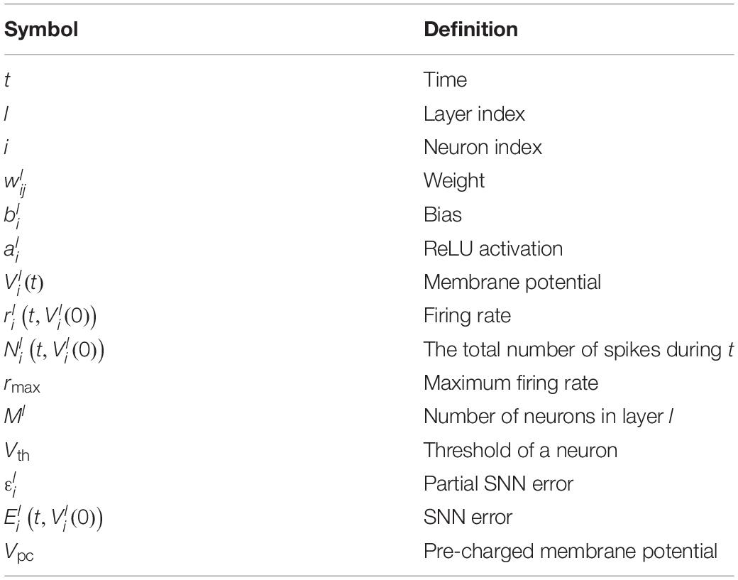
Table 1. Definition of symbols.

$$r_i^0(t,V_i^0(0))=a_i^0-\frac{V_i^0(t)-V_i^0(0)}{t}.(3)$$

For consistency, we assume that the input spikes are generated by the same method as in the other neural network layers. Starting with Eq. (3), we can recursively expand Eq. (2) as,

$$r_i^l(t,V_i^l(0))=a_i^l+{\mathrm{\epsilon }}_i^l+\sum _{i_{l-1}=1}^{M^{l-1}}{w}_{i_l{i}_{l-1}}^l{\mathrm{\epsilon }}_{i_{l-1}}^{l-1}+\mathrm{\cdots }+\sum _{i_{l-1}}^{M^{l-1}}{w}_{i_l{i}_{l-1}}^l\mathrm{\cdots }$$

$$\sum _{i_0=1}^{M^0}{w}_{i_1{i}_0}^1{\mathrm{\epsilon }}_{i_0}^0.(4)$$

Here, if ${\sum }_{j=1}^{M^{l-1}}{w}_{ij}^l{r}_j^{l-1}(t,V_i^l(0))+r_{\max }{b}_i^l>0$, a partial error ${\mathrm{\epsilon }}_i^l$ is $-\frac{V_i^l(t)-V_i^l(0)}{t}$; otherwise, it is zero since the neuron does not generate any spike. From Eq. (4), we can define an SNN error as,

$$E_i^l(t,V_i^l(0))=r_i^l(t,V_i^l(0))-a_i^l={\mathrm{\epsilon }}_i^l+\sum _{i_{l-1}=1}^{M^{l-1}}{w}_{i_l{i}_{l-1}}^l{\mathrm{\epsilon }}_{i_{l-1}}^{l-1}+\mathrm{\cdots }+$$

$$\sum _{i_{l-1}=1}^{M^{l-1}}{w}_{i_l{i}_{l-1}}^l\mathrm{\cdots }\sum _{i_0=1}^{M^0}{w}_{i_1{i}_0}^1{\mathrm{\epsilon }}_{i_0}^0.(5)$$

Eq. (5) says that the SNN error of layer l is the sum of the partial error generated in that layer and the partial errors generated at and propagated through the previous layers.

Up to the present, it has been customary to set all initial membrane potentials, $V_i^l(0)$, to zero before the inference starts. If $V_i^l(0)=0$, however, the partial error, ${\mathrm{\epsilon }}_i^l$, is always negative, resulting in the inherent latency of SNN. If we set $V_i^l(0)$ to some positive value, V_pc (< V_th), it corresponds to PCMP. Since $\frac{V_{\text{pc}}}{t}$ will compensate the negative value of the term, $\frac{V_i^l(t)}{t}$, it can have a strong impact on the SNN error during the initial transient.

Some studies have reported that the method of lowering V_th to reduce the latency by increasing the firing rate (Diehl et al., 2015; Park et al., 2019). As shown in Eq. (2), the decrease of V_th without considering the threshold balancing leads to the increase of the steady-state firing rate, resulting in a large error propagating to the subsequent layers. Thus, the degradation in the steady-state of performance can occur. However, from Eq. (4), we can notice that PCMP does not alter the steady-state firing rate because ${\mathrm{\epsilon }}_i^l$ decays to zero as the inference time increases. In other words, PCMP only induces an earlier firing of the first spike. If the integration starts from V_pc, the potential required to reach the threshold of a neuron (V_th) is reduced to V_th −V_pc, resulting in earlier firing of the first spike. After the first spike, the membrane potential is reset by subtraction so that the neuron starts to generate spikes with almost regular time interval (Rueckauer et al., 2017). Therefore, PCMP is powerful in that it only can reduce the latency without violating the equivalence condition between the ANN activations and the firing rates of SNN.

On the other hands, the firing rate $r_i^l(t,V_i^l(0))$ generates low-precision information and contains a considerable error at the early timesteps based on Eq. (4). As mentioned in Eq. (5), the error propagates to the subsequent layers multiplied by the weights, so it becomes significantly large in the output layer. Of course, the first few spikes play a significant role in biological nerve systems, and other spike coding methods such as temporal or first-time-to-spike coding are actively studied (Rullen and Thorpe, 2001; Park et al., 2020); however, it is likely that the initial few spikes occurring in the output neurons entail inaccurate information when rate-based coding is used. Thus, we try to discard the error spikes at the early timesteps by giving deliberate delay in the output neurons, referred as a DE. This method can be utilized in combination with PCMP to achieve further latency reduction.

Network Architecture

Firstly, we train a network composed of 3C20-5C50-FC50-FC10 for MNIST classification, referred as Net 1. nCm(s) represents n × n convolution operation with m filters and stride s, and FCn means a fully connected layer with n neurons. Dropout technique is employed with the probability of 50%, and the adaptive learning rate by multiplying 0.1 after 60, 120, and 180 epochs with the initial value of 1 × 10^–3 is applied. Weights are optimized by Adam with L2 decay parameter of 1 × 10^–4. After training, a test accuracy of 99.35% is achieved.

Net 2 is an all convolutional network consisting of 3C96-3C96(2)-3C192-3C192-3C192(2)-3C192-1C192-1C10-GAP where GAP denotes for global average pooling (Springenberg et al., 2014). Some nodes are randomly dropped out with the probability of 50% for generalization, and the adaptive learning rate by multiplying 0.5 after 50, 100, and 200 epochs with the initial value of 1 × 10^–3 is applied. Stochastic gradient descent (SGD) algorithm is utilized for optimization. The classification accuracy of 91.77% is obtained for test dataset.

In order to demonstrate the effect of the proposed methods on general SNN applications, Net 3 is trained as an autoencoder. The structure is 3C96-3C96(2)-3C32(2)-3C16(2)-3C^T32(2)-3C^T96(2)-3C^T96(2)-3C^T3 where nC^Tm(s) represents m transposed convolution filters of size n × n. CIFAR-10 dataset is employ to train the network with Adam optimizer and the adaptive learning rate by multiplying 0.1 after 120, 240, and 360 epochs with the initial value of 1 × 10^–3. Lena image (512 × 512) split into 256 of 32 × 32 patches is used as a test sample for inference. Detailed training method and hyper parameters are based on the previous work (Hwang et al., 2020).

The trained weights are normalized by “Data-based Normalization” and transferred to SNNs (Diehl et al., 2015). We employ the rate-based coding to represent ANN input activations by applying constant current inputs to the integrate-and-fire neurons. The simulation timestep is divided to simulate the SNNs most efficiently in the aspect of the computing complexity so that a neuron with the highest firing rate generates spikes in every timestep. The ANN-to-SNN conversion used in this work is based on the previous work (Rueckauer et al., 2017).

Results

Latency of SNNs

The classification accuracy and MSE of SNNs according to the simulation timestep for Net 1 ∼ 3 are shown in Figures 1A,B, respectively. As the simulation time increases, the performance of SNNs increases as well, and it converges to the ANN’s performance. As shown in Figure 1A, for Net 1, which represents a relatively simple network, it reaches ANN’s accuracy within a small number of timesteps; however, in a much deeper network, such as Net 2, the latency becomes severely worse resulting in a longer convergence time. We also extract MSE of Net 3 between the SNN firing rate and ANN’s activation in the output layer, so zero MSE means that the SNN’s output equals to the ANN’s output. As illustrated in Figure 1B, MSE of Net 3 gradually decreases with respect to the number of timesteps, but MSE does not reach ANN’s performance within 255th timestep.

FIGURE 1

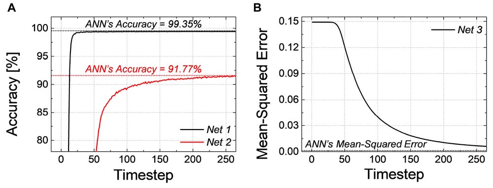
Figure 1. (A) Accuracy of Net 1, 2 and (B) MSE of Net 3 according to the simulation timestep. Time to reach ANN’s performance is required because of the latency of SNN.

The latency of SNN can be observed in < f_SNN > _norm, the averaged firing rate over all test samples normalized by ANN’s activation. < f_SNN > _norm of Net 1 ∼ 3 in the input and output layers according to the simulation timestep are shown in Figures 2A–C, respectively. If < f_SNN > _norm converges to one, it indicates that the performance of SNNs becomes equivalent to that of ANNs. We can see that even < f_SNN > _norm of the input layer has some latency until it converges to one (it is quite small in Net 1, but very conspicuous in Net 2 and 3). < f_SNN > _norm of the output layer is lagging behind that of the input layer due to the latency, and it is worse in the deep and complex network like Net 2 and 3.

FIGURE 2

Figure 2. < f_SNN > _norm, the averaged firing rate over all the test samples normalized by ANN’s activation in the input and output layers according to the simulation timestep for (A) Net 1, (B) Net 2, and (C) Net 3. < f_SNN > _norm of the output layer suffers from the latency compared with that of the input layer.

Pre-charged Membrane Potential

Firstly, we have simulated the effect of PCMP by applying the global PCMP (the same initial membrane potential, V_pc, to all neurons in the network). Figure 3A illustrates the classification accuracy as a function of simulation time for Net 1, while varying V_pc from 0.0 to 0.5 with 0.1 steps. As V_pc increases, there seems fast convergence to the ANN’s accuracy in that the accuracy vs. time curve shifts to the left. In order to precisely estimate the latency reduction, the number of timesteps to reach 99.0, 99.5, and 99.9% of the ANN’s accuracy (denoted as t_99.0, t_99.5, and t_99.9%) are extracted, as shown in Figure 3B. The timestep to reach 99.0 and 99.5% of the ANN’s accuracy is decreased with the increase of V_pc from 0.0 to 0.5. If the criterion of latency is raised to 99.9% of the ANN’s accuracy, PCMP up to 0.3 reduces the latency while too much PCMP increases it. PCMP can substantially improve the convergence time so that we can obtain the best latency reduced by 59% for t_99.0% (@V_pc of 0.5), 43% for t_99.5% (@V_pc of 0.5) and 25% for t_99.9% (@V_pc of 0.3) compared with the case without PCMP (@V_pc of 0.0). Figure 3C shows < f_SNN > _norm of Net 1 in the output layer with respect to the different levels of V_pc. The point of the rapid rise in < f_SNN > _norm moves to the left as V_pc increases, but too much V_pc induces over-firing during the early timesteps, which can rather degrade the latency.

FIGURE 3

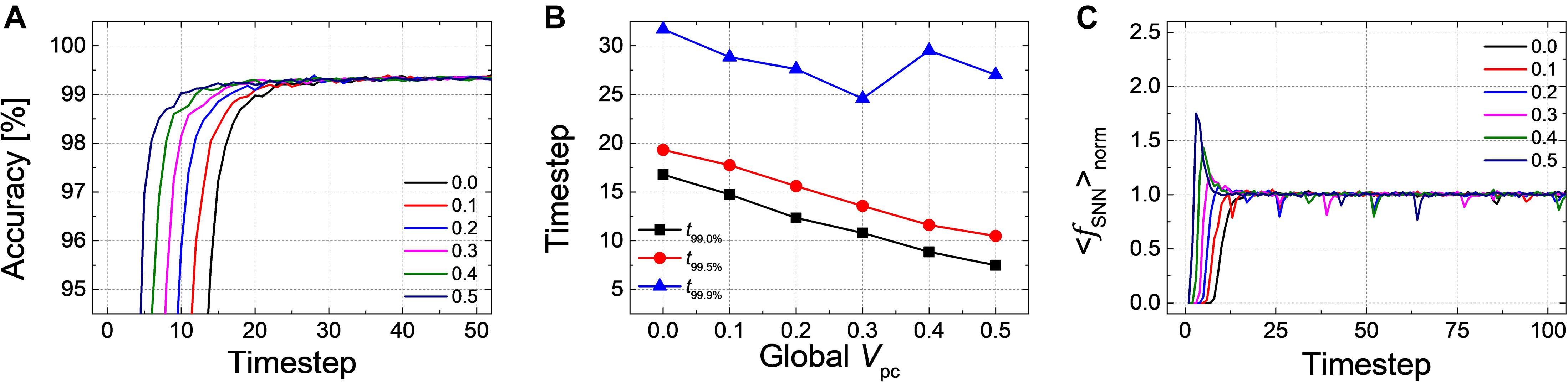
Figure 3. (A) Result of accuracy-timestep for Net 1 with the global V_pc varying from 0.0 to 0.5 with 0.1 steps. (B) Extracted timesteps (t_99.0%, t_99.0%, and t_99.9%) with respect to the amount of the global V_pc. (C) The average firing rate in the output layer with the different levels of the global V_pc according to the simulation timestep.

In addition, correlation diagrams which reveal that V_pc facilitates the rapid inference in SNNs by reducing inherent delay are extracted in Figure 4. How precisely the firing rates of SNNs reproduce the ANN activations can be analyzed through the correlation diagram, where an ANN activation of a neuron is on x-axis while its SNN firing rate is on y-axis (Rueckauer et al., 2017; Hwang et al., 2020). If the SNN firing rate is perfectly reproduce the ANN activation for all neurons, all points in the correlation diagram are on line (y = x); however, when there is the latency, the firing rate of SNNs falls behind the activation of ANNs; thus, the points on the correlation diagram are positioned below the line of perfect correlation (y = x). The correlation diagrams are extracted from all neurons in the network using test dataset at 50, 100, and 150th timesteps with V_pc of 0.0 and 0.5, as shown in Figures 4A,B, respectively. In both cases, the firing rates of the neurons close to the input layer correlate quite well with the ANN activations even at the early time. As the simulation time increases, the firing rates of the neurons close to the output layer converges to the ANN activations, so that the points tend to be on the line (y = x); however, the increase of the slope is much faster for V_pc of 0.5. The slope of the correlation diagram of the output layer for V_pc of 0.0 is still less than one at the 150th timestep, showing that there still remains some delay.

FIGURE 4

Figure 4. Correlation plots of Net 1 at 50, 100, and 150th timesteps for the global V_pc of (A) 0.0 and (B) 0.5. The latency occurs in early timestep, and its effect gradually disappears along with the simulation time. Latency reduction effect is more noticeable when the global V_pc of 0.5 is applied.

For Net 2, Figure 5A shows the changes of the classification accuracy according to the inference time with the different levels of V_pc. The time-accuracy curve prominently shifts to the left with the increase of V_pc from 0.0 to 0.3 while it goes back to the right when V_pc above 0.3 is applied. The timestep when the accuracy reaches to 99.0, 99.5, and 99.9% of the ANN’s accuracy is extracted with respect to the changes of V_pc in Figure 5B. Compared with the case without V_pc, the best latency is reduced by 19% for t_99.0% (@V_pc of 0.3), 13% for t_99.5% (@V_pc of 0.2), and 13% for t_99.9% (@V_pc of 0.3). The convergence time is increased when V_pc above a certain value is applied. < f_SNN > _norm in the output layer for Net 2 with respect to the different levels of PCMP from 0.0 to 0.5 is illustrated in Figure 5C. The early rising of < f_SNN > _norm is observed as V_pc increases; however, for the case with V_pc above 0.3, there occurs a fluctuation by over- and under-firing caused by too much PCMP, which is the cause of the increase in the latency.

FIGURE 5

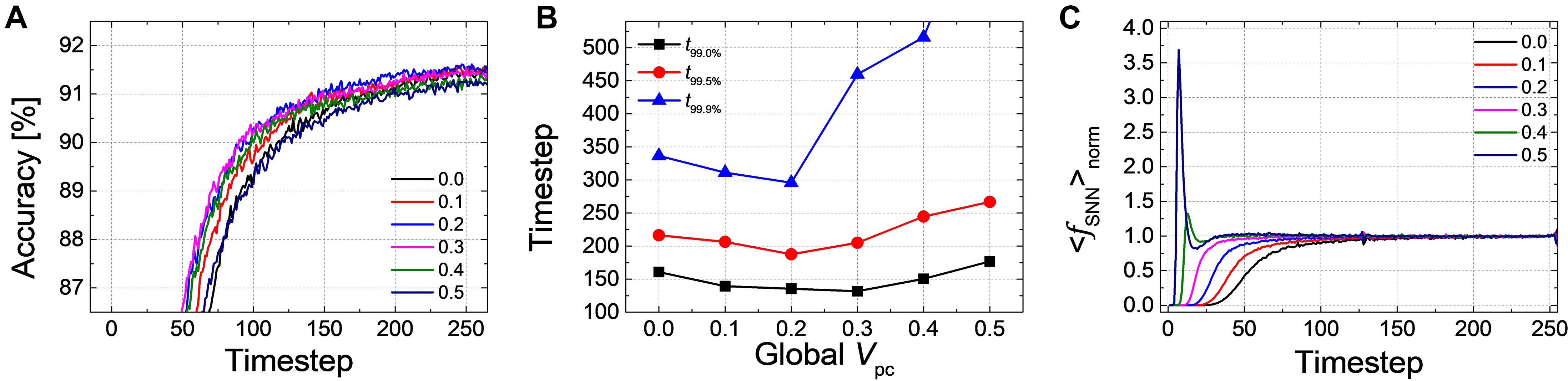
Figure 5. (A) Accuracy-timestep result for Net 2 with the global V_pc changing from 0.0 to 0.5 with 0.1 steps. (B) Extracted timestep to reach 99.0, 99.5, and 99.9% of the ANN’s accuracy according to the changes of the global V_pc. (C) The average firing rate in the output layer with different level of the global V_pc according to the simulation timestep. It is noticeable that the point of timestep in which the firing rate rises becomes earlier.

The correlation diagrams of Net 2 show the effect of the latency reduction more clearly than that for Net 1. Figures 6A,B represent the correlation diagrams of all neurons at the 100, 250, and 750th timesteps using all test data with V_pc of 0.0 and 0.3, respectively. In deep SNNs, as expected, the latency appears more pronounced for the neurons closer to the output layer, as illustrated in Figure 6A. The firing rates gradually increases so that it approaches the ANN activations, but it takes more time compared with the case of Net 1. The slope quickly reaches to one for V_pc of 0.3 compared with the case for V_pc of 0.0. Eventually, all the points are well-correlated to the ANN’s activations for the case using V_pc of 0.3 at the 750th timestep, while the latency still remains in the case of V_pc of 0.0 at the same timestep.

FIGURE 6

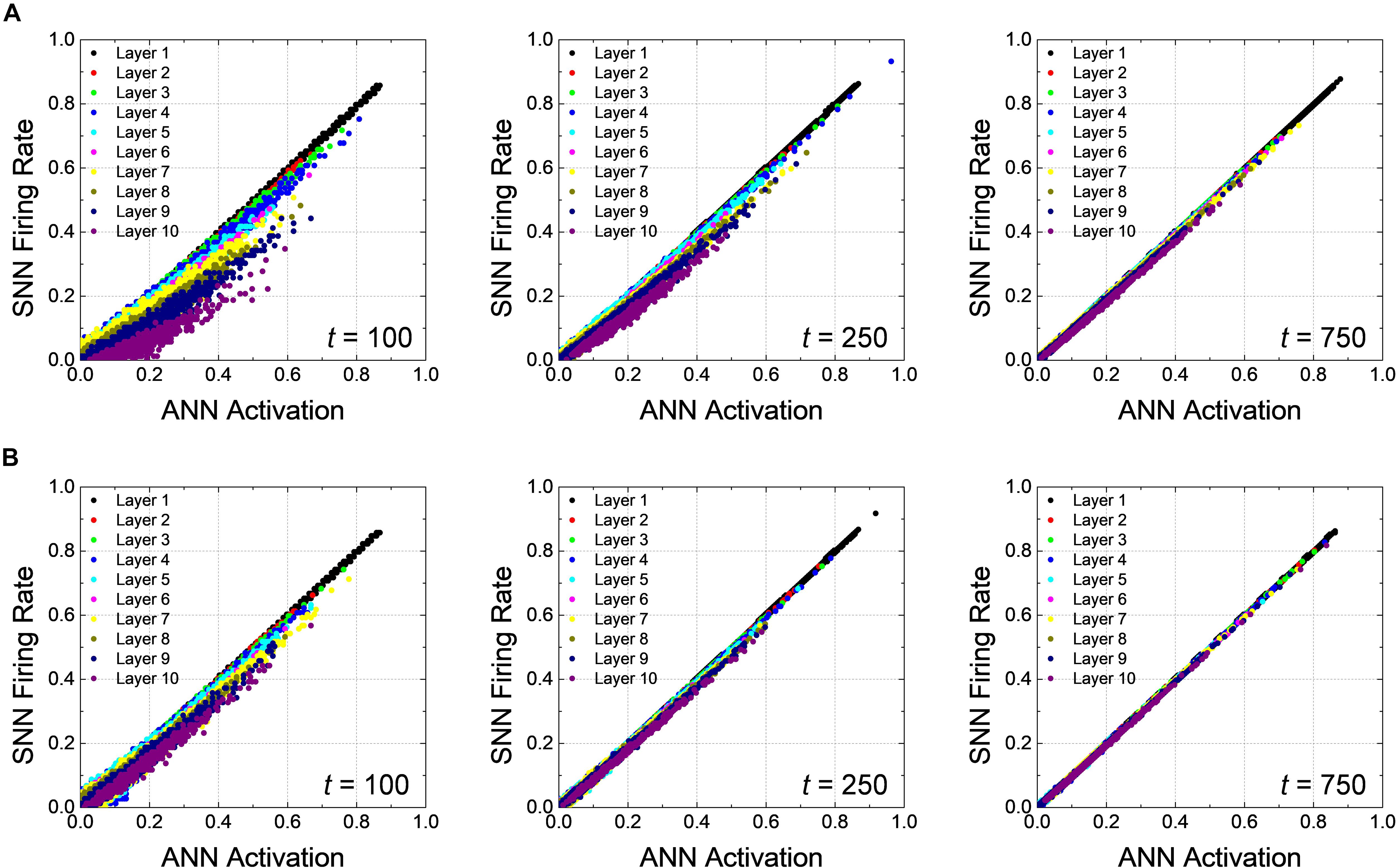
Figure 6. Correlation diagrams of Net 2 at 100, 250, and 750th timesteps for the global V_pc of (A) 0.0 and (B) 0.3. In a deep network, the latency is more clearly seen compared with the case of Net 1.

Pre-charged membrane potential is effective to reduce the latency as well not only for a classification problem but also for an autoencoder as Net 3. In particular, unlike the classification problems in which the relative number of output spikes matters, the absolute firing rate itself is of importance in autoencoder. Figure 7A shows the changes of MSE as a function of the inference time in the output layer with V_pc varying from 0.0 to 0.5. MSE gradually decreases as a function of the inference time, but it converges much faster when the amount of PCMP increases. The early firing of spikes and fast convergence are also observed by < f_SNN > _norm with respect to the inference time for the output layer with the different levels of PCMP, as shown in Figure 7B. The changes of a decompressed image in the output layer at the 50, 100, 150, 200, and 255th timesteps for V_pc of 0.0 and 0.5 are shown in Figures 7C,D, respectively. In both cases, the images at the 255th timestep are successfully restored close to the original image; however, compared with the images using V_pc of 0.0, the images using V_pc of 0.5 become similar to the original image more quickly.

FIGURE 7

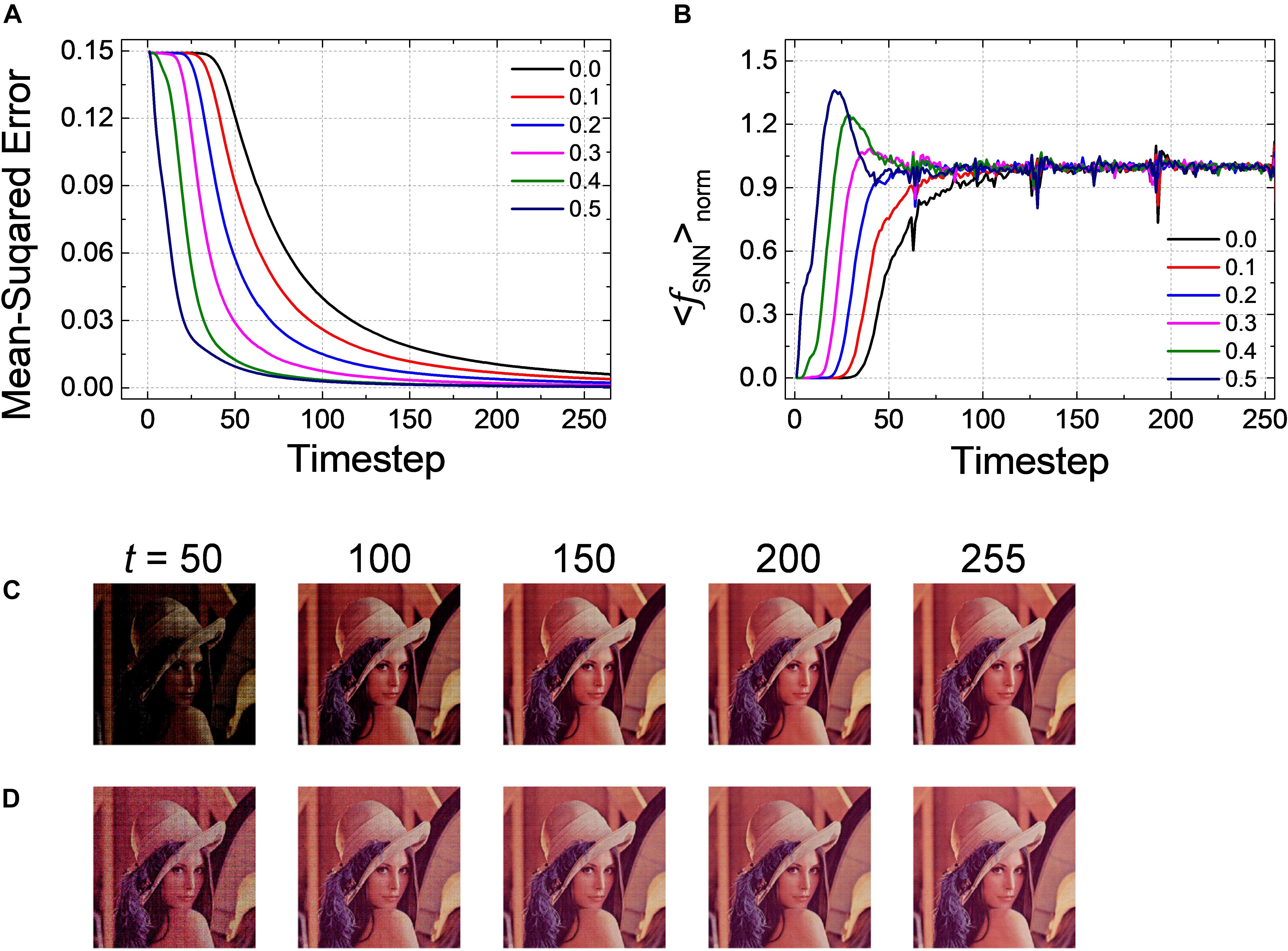
Figure 7. (A) Changes of MSE for Net 3 when increasing the amount of the global V_pc from 0.0 to 0.5 with 0.1 steps. MSE decreases more quickly as the global V_pc increases. (B) The average firing rate in the output layer with the different levels of the global V_pc according to the simulation timestep. Restored sample image in the output layer of Net 3 at 50, 100, 150, 200, and 255th timestep for the global V_pc of (C) 0.0 and (D) 0.5.

Optimization of Pre-charged Membrane Potential

The global PCMP that applies the same amount of V_pc to all neurons in the network is a practical approach because of its simplicity, but we may optimize the amount of PCMP layer by layer. Brute-force layer-wise optimization, however, requires extraordinary computational power. For example, if there are 10 layers and 10 possible V_pc values for each layer, we have to check 10¹⁰ cases, each of which would take at least 10 s with the help of a powerful graphical processing unit (GPU). The total amount of time we have to devote for this task would be more than 300 years.

Based on the observation that the SNN error, $E_i^l(t,V_i^l(0))$, depends on the partial errors, ${\mathrm{\epsilon }}_i^l$, for l ∈ {0,…,L}, we have devised a sequential layer-wise optimization method. Here, we assume that all the neurons in layer l have the same initial membrane potential, so $V_i^l(0)$ can be denoted as V^l. For layer-wise optimization, we define the mean-squared SNN error ⟨[E^l(t,V^l)]2⟩ in layer l for the training set, which is expressed as

$$⟨{[E^l(t,V^l)]}^2⟩=\frac{\sum _{i=1}^{M^l}{[E_i^l(t,V^l)]}^2}{M^l}(6)$$

As a first step, ⟨[E⁰(t,V⁰)]²⟩ is extracted by changing the initial membrane potential V⁰ from 0.0 to 0.5 with 0.01 steps. Then, V⁰ which minimizes the time sum of ⟨[E⁰(t,V⁰)]²⟩ during 1-epoch is determined as the optimal $V_{\text{pc}}^0$. Here, 255^th timestep is defined as one-epoch because the precision of the input image is eight-bit, so the input image is completely applied to the network at 255th timestep. This procedure can be repeated sequentially from the input to output layers. The point is that the optimization in layer l must be performed with the all the optimal PCMP in the previous layers ($V_{\text{pc}}^0,V_{\text{pc}}^1,\mathrm{\cdots },V_{\text{pc}}^{l-1}$) applied. The layer-wise optimization procedure is described in Algorithm 1.

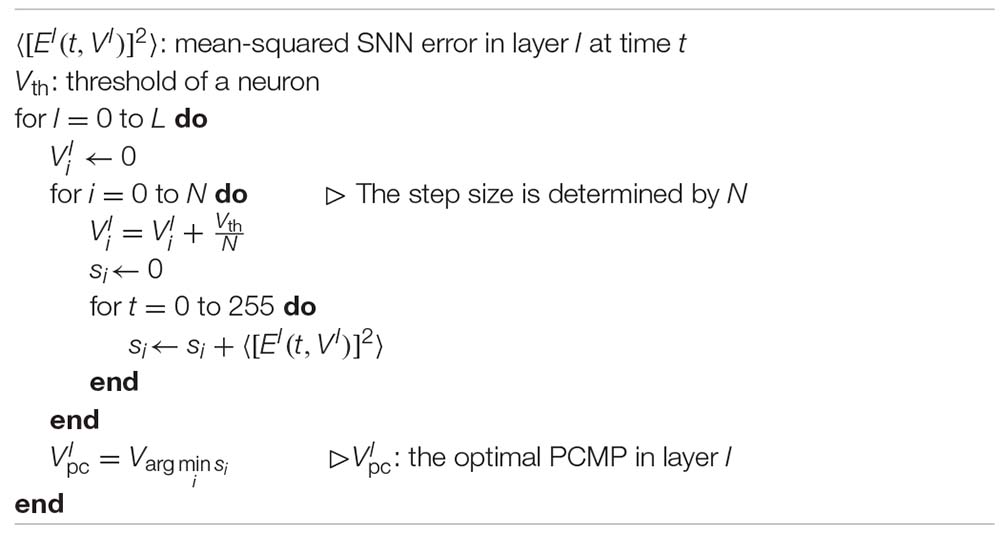
Algorithm 1: Layer-Wise Optimization

We conduct the layer-wise optimization, and the time sum of ⟨[E^l(t,V^l)]²⟩ for Net 1 ∼ 3 at l=1, as an example, is extracted according to PCMP in Figures 8A–C, respectively. It can be seen that the time sum of ⟨[E^l(t,V^l)]²⟩ decreases and then increases, so there is the global minimum of V^l which is determined as the optimal $V_{\text{pc}}^l$. Figures 9A–C describe the changes of MSE between the SNN firing rates and ANN activations in the output layer of Net 1 ∼ 3 over the simulation time by applying the global PCMP and the layer-wise optimization, respectively. It is confirmed that the layer-wise optimization results in a fast decrease of MSE compared with the case of the global PCMP. The latency of Net 1 and 2 is summarized in Table 2, and the best record is marked in bold with ^∗. In classification problems, it is found that a fast decrease in MSE does not necessarily guarantee rapid convergence in the accuracy since the accuracy is determined by comparing the relative number of spikes among the output neurons.

FIGURE 8

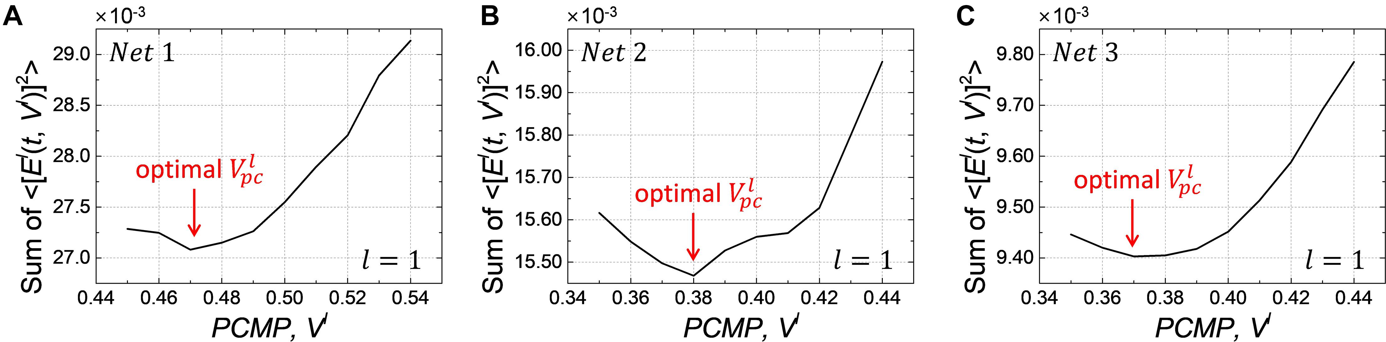
Figure 8. Changes of the time sum of ⟨[E^l(t,V^l)]²⟩ in layer l=1 when increasing the amount of PCMP, V^lfor (A) Net 1, (B) Net 2, and (C)Net 3. The optimization process is conducted from the input to the output layer sequentially, and it also needs to keep the optimized PCMPapplied to the previous layers when performing the optimization for the subsequent layers.

FIGURE 9

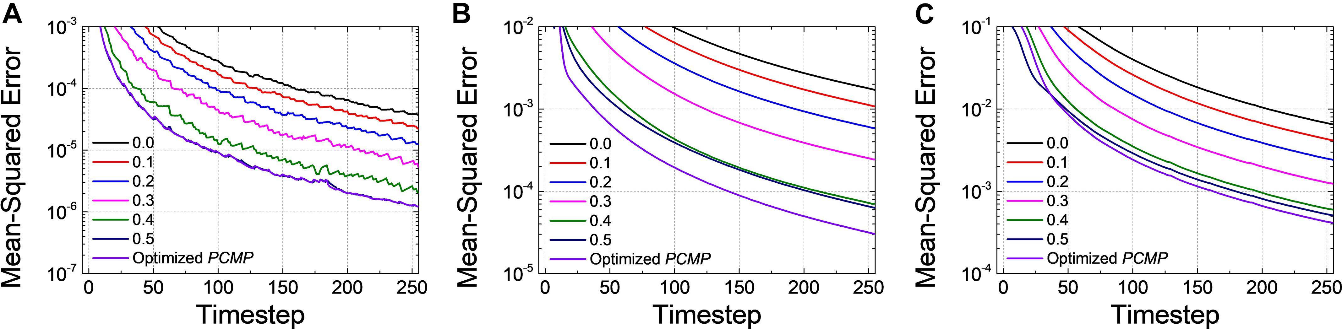
Figure 9. Changes of MSE for (A) Net 1, (B) Net 2, and (C) Net 3 when increasing the amount of the global V_pc from 0.0 to 0.5 with 0.1 steps and the optimized PCMP. Although the global PCMP is practical due to its simplicity, the layer-wise optimization is more effective in a fast decrease of MSE.

TABLE 2

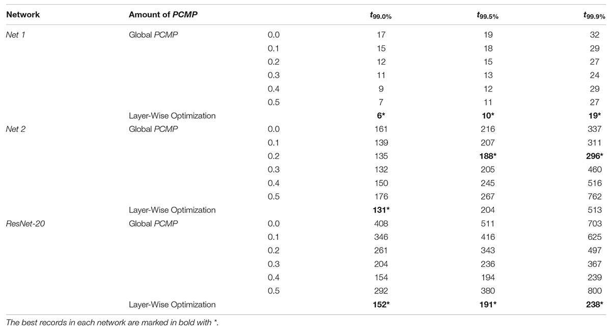
Table 2. Latency of Global PCMP and Layer-Wise Optimization for Net 1, Net 2, and ResNet-20.

Delayed Evaluation

There is a great fluctuation in the SNN error, $E_i^l(t,V_i^l(0))$, during the initial timesteps. This is because the firing rate of input spikes has not reached the steady-state value. That is, a transient appears at the initial timesteps for SNNs. Spikes can be under-fired or over-fired during the initial transient, which contributes to the spike rate as significant errors. Therefore, if the inference operation is intentionally delayed in the output layer to eliminate the errors in the spike rate during the initial transient, fast and accurate inference operation can be achieved. We call this inference method as a DE.

As an example, the classification accuracy according to the simulation time for Net 2 with DE of 40-timestep and without DE is illustrated in Figure 10A. During the intentional delay, the inference is not performed, so the classification accuracy cannot be extracted; however, it rapidly increases and converges to the ANN’s accuracy after the intentional delay. It may appear that the case with DE converges slower than that without DE, but if we closely examine the accuracy curves near the point where they cross each other, the accuracy with DE rapidly surpasses that without DE, as shown in the inset of Figure 10A. The effect of DE is also verified in Net 3. Figure 10B illustrates the changes of MSE with DE of 50-timestep and without DE. MSE remains constant during the early timesteps. Once the evaluation starts, however, MSE with DE decreases and approaches zero much faster than that without DE.

FIGURE 10

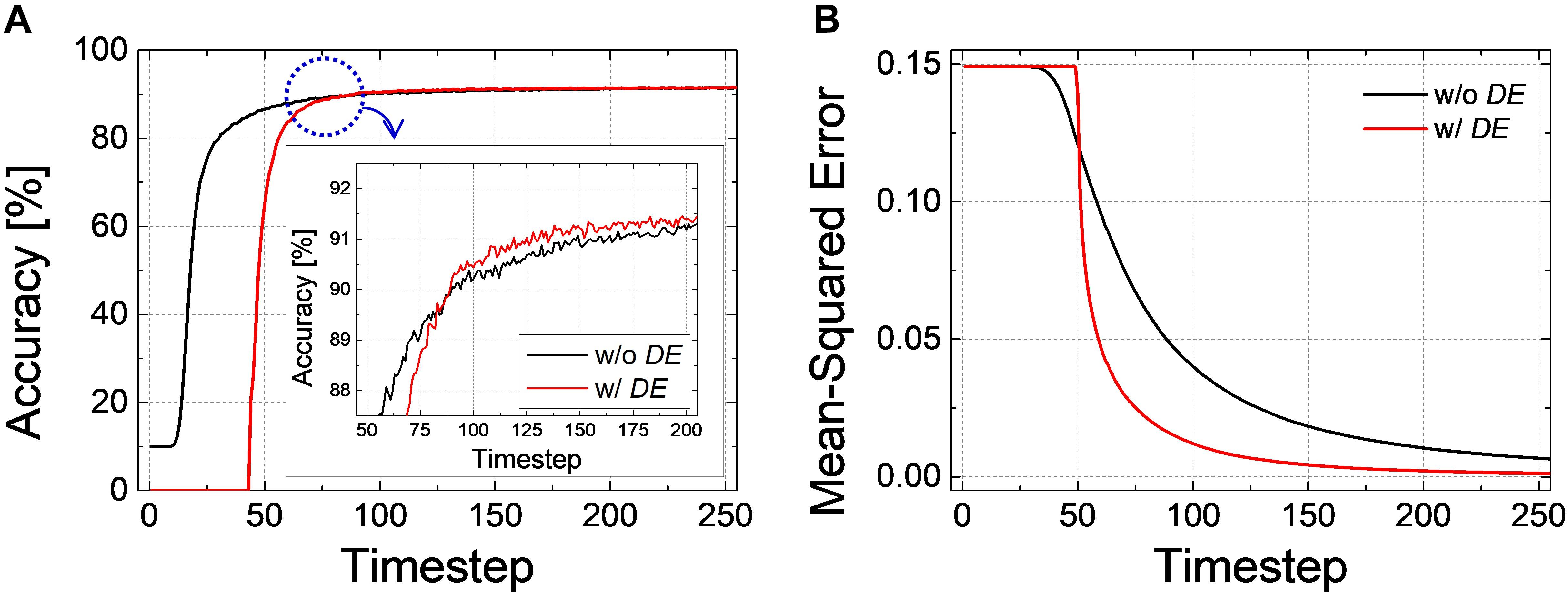
Figure 10. (A) Accuracy-timestep curve of Net 2 with- and without DE. Both cases converge to the ANN’s performance, but the accuracy with DE converges faster than that without DE. (B) Changes of MSEwith respect to the simulation timestep for Net 3 with- and without DE. MSE with DE decreases and approaches zero much faster than that without DE.

We have investigated the inference performance by varying the intentional delay of DE. For example, Figure 11A shows the changes of timestep to reach 99.0% of the ANN’s accuracy (t_99.0%) for Net 1 with global and optimized PCMP. Firstly, t_99.0% shows no change when the intentional delay is short. In classification problems, the output neuron firing the most is considered as the correct answer; there is a period of time when no spike is generated in the output layer, so an intentional delay shorter than this “no-spike” period will not change the most-firing neuron; therefore, no change of accuracy is observed. If the intentional delay increases, however, t_99.0% increases as if it is pushed up by the excessive intentional delay. Even if the SNN is very close to the steady state, the evaluation time should be sufficiently long to achieve high accuracy; otherwise, the number of spikes corresponding to a low ANN activation would be too small for accurate evaluation. We can call this period of time “excessive intentional delay” period. The latency reduction by DE does not appear since Net 1 has a short latency due to the relatively simple network structure and data to classify.

FIGURE 11

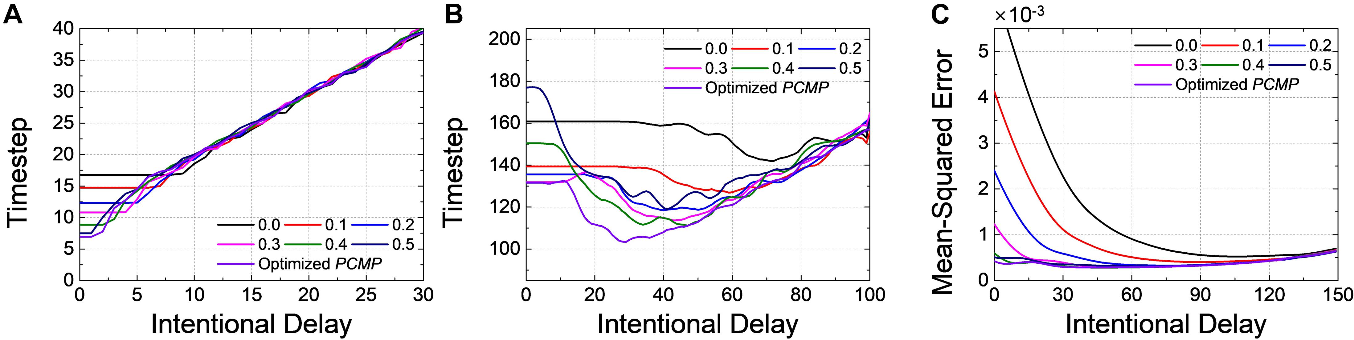
Figure 11. Changes of timestep when 99.0% of the ANN’s accuracy is reached with respect to the intentional delay for (A) Net 1 and (B) Net 2. Changes of MSE at 1-epoch (255th timestep) for (C) Net 3. Different levels of the global and the optimized PCMP are used for Net 1 ∼ 3. Delayed evaluation (DE) is effective to achieve the further reduction of the latency, and it can be applicable simultaneously with PCMP.

For Net 2 with global and optimized PCMP, t_99.0% is extracted with respect to the intentional delay, as shown in Figure 11B. As mentioned above in Figure 11A, there occurs “no-spike” period as well in Net 2. After the no-spike period, spikes start to be generated in the output layer, but the spike rate is still incorrect. By DE, we can remove errors in the spike rate, which helps to decrease t_99,0%. Thus, this period of time where t_99.0% decreases is referred as “error removal” period. Here, we can notice that that the combined use of PCMP and DE is significantly effective in reducing the latency. With large the intentional delay, however, t_99.0% suffers from “excessive intentional delay” period, it is dominated by the intentional delay.

For Net 3 with global and optimized PCMP and MSE at 1-epoch (255th timestep) is extracted by changing the intentional delay, as illustrated in Figure 11C. Unlike the classification problem, MSE decreases rapidly with the increase of DE. Since DE excludes a chunk of “no-spike” period in evaluation, the output spike rates get closer to the target spike rates rapidly. As DE increases further, however, MSE remains more or less constant. This is because the precision reduced by DE induces errors, but there is also the error reduction due to the removal of the initial transient. Those effects cancel each other out, resulting in little changes of MSE. After that, MSE increases since it starts to be in “excessive intentional delay” period.

Effects on ResNet-20

In order to demonstrate the effectiveness of the proposed methods in much deeper and most generally used neural network models, we train ResNet-20 using CIFAR-10 dataset (He et al., 2016). Firstly, the network is trained by SGD algorithm with the momentum of 0.9 and L2 weight decaying parameter of 1 × 10^–4. Adaptive learning rate is employed with the initial learning rate of 0.1, so it is multiplied by a factor of 0.1 after 82, 123, and 164 epochs. Also, 32 × 32 random cropping (padding = 4) and the horizontal flipping are used for data augmentation. We can obtain the accuracy of 91.82% for the test dataset. The trained network is converted to SNN using the weight normalization method of ResNet which has been already reported in the previous research (Hu et al., 2018).

Figure 12A shows the accuracy of the spiking ResNet-20 according to the simulation timestep with the different value of the global PCMP. When increasing the global PCMP from 0.0 to 0.4, the curve shifts to the left, and it goes back to the right when the global PCMP of 0.5 is applied. We extract t_99.0, t_99.5, and t_99.9% with the different amount of the global PCMP, as illustrated in Figure 12B. For all criteria, it is found that the convergence time decreases with the increase of the global PCMP up to 0.4 and increases again at the global PCMP of 0.5. Figure 12C indicates the result of MSE in the output layer when the layer-wise optimization is performed. MSE with the optimized PCMP appears smaller than that with the global PCMP. The best records of the latency in ResNet-20 with PCMP are summarized in Table 2. We also perform the DE in ResNet-20, and t_99.0% is extracted with respect to the intentional delay, as shown in Figure 12D. It is confirmed that the convergence time remains the same during “no-spike” period, decreases during “error removal” period, and increases during “excessive intentional delay” period. These results are consistent with the results above; therefore, the effectiveness of the proposed methods is successfully demonstrated in much deeper networks.

FIGURE 12

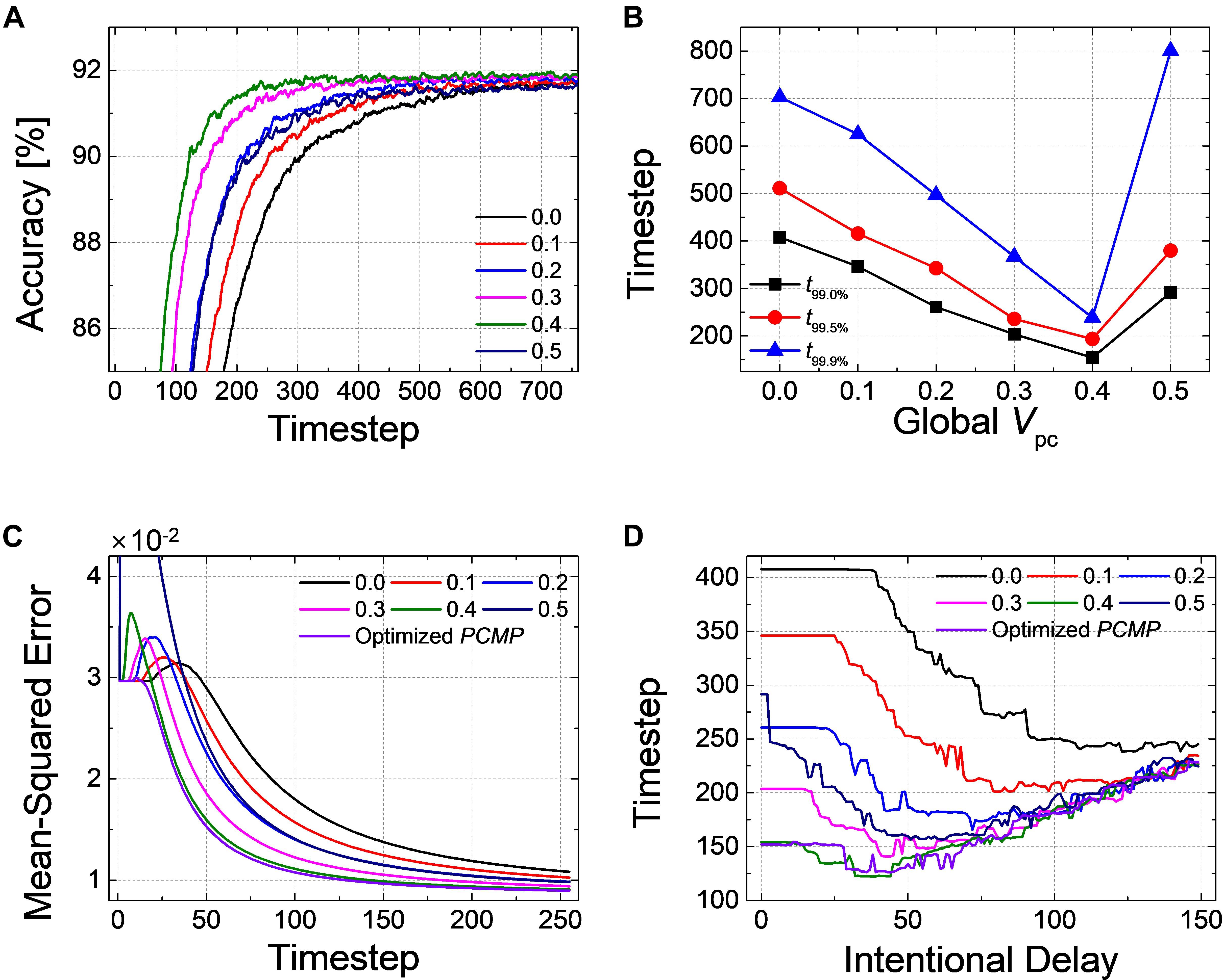
Figure 12. Effects of the proposed methods on ResNet-20. (A) Changes of the classification accuracy according to the global V_pc from 0.0 to 0.5. (B) Extracted timesteps (t_99.0%, t_99.0%, and t_99.9%) with respect to the amount of the global V_pc. (C) Changes of MSE for when increasing the amount of the global V_pc from 0.0 to 0.5 with 0.1 steps and the optimized PCMP. (D) Changes of timestep when 99.0% of the ANN’s accuracy is reached when using DE.

Discussion

Reduction of Computational Cost

The one of the most powerful advantage in using SNN is that energy-efficient inference is possible due to its event-driven characteristic. SNN updates its state when there is spike; therefore, the computational cost is proportional to the number of synaptic operations, which can be approximated by the number of spikes when performing the inference. Reducing the latency of SNN can contribute to saving of the number of synaptic operations required to determine the result. In order to confirm the advantage of the proposed methods in terms of the computation cost, we extract the number of synaptic operations per image (SOPs/image) for Net 1 ∼ 3, as shown in Figure 13. For classification problems such as Net 1 and 2, SOPs/image is extracted based on the latency to reach 99.0, 99.5, and 99.9% of the ANN’s accuracy (t_99.0, t_99.5, and t_99.9%). In the case of autoencoder, such as Net 3, MSE at 1-epoch is set as a reference when neither PCMP nor DE is applied, and SOPs/image is extracted based on the latency to reach the reference MSE.

FIGURE 13

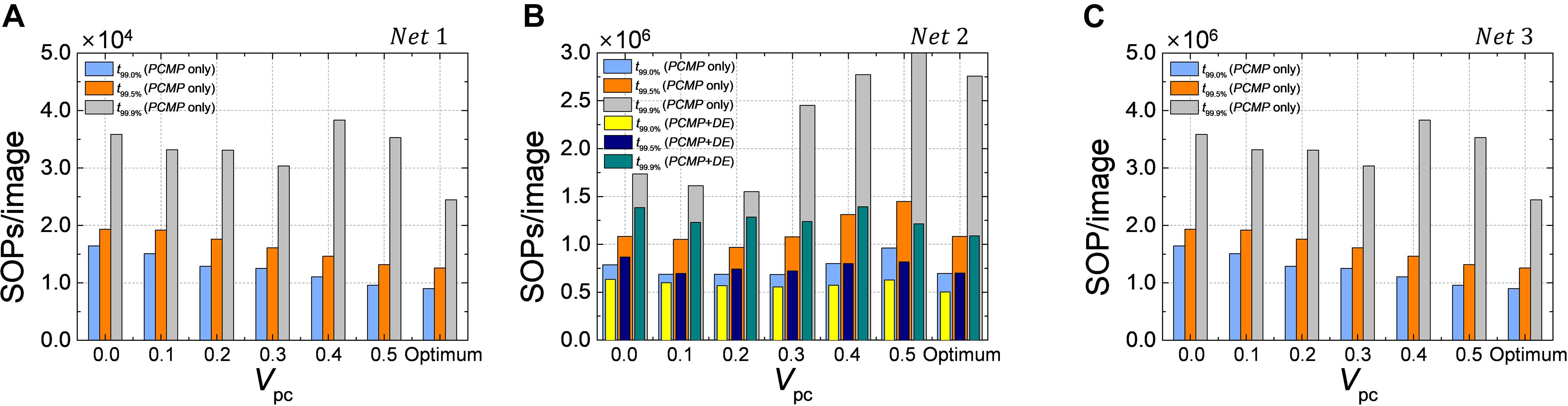
Figure 13. The number of synaptic operations per image (SOPs/image) for (A) Net 1, (B) Net 2, and (C) Net 3. SOPs/image is extracted based on t_99.0%, t_99.0%, and t_99.9% in the classification problems and on the reference MSE (MSE@1-epoch without PCMP and DE). The effect of the proposed methods for energy-efficient computing is remarkable.

Because DE has no effect on the latency reduction in Net 1, Figure 13A shows SOPs/image for Net 1 only using the global PCMP (0.0 ∼ 0.5) and optimized PCMP by the layer-wise optimization. It is clearly confirmed that the latency reduction by PCMP leads to the reduction of SOPs/image. The best computational cost is obtained when the layer-wise optimization of PCMP is performed, where it is reduced by 46, 35, and 32% for t_99.0, t_99.5, and t_99.9%, respectively, compared with the case without PCMP and DE. For Net 2, as shown in Figure 13B, when only PCMP is applied, the best SOPs/image is obtained at V_pc of 0.2 for t_99.9 and t_99.5% and at the optimized V_pc for t_99.0%, which are reduced by 11, 11, and 12%, respectively, compared with the case without PCMP. Moreover, it is obviously demonstrated that the combination of PCMP and DE has a significant effect on reducing the computation cost so that it helps to reduce SOPs/image by 37, 36, and 38% for t_99.0, t_99.5, and t_99.9%, respectively, compared with the case without PCMP and DE. The effect of PCMP and DE on the reduction of the computational cost is verified as well in the autoencoder, Net 3, the best SOPs/image to reach the reference MSE is reduced by 74% when the optimized V_pc and DE are applied, as shown in Figure 13C.

Comparison With Prior Work

Table 3 shows the comparison results with the prior work in terms of dataset, spike encoding, accuracy, architecture, accuracy, and the latency. In the previous research implementing CNN through rate-based coding, the latency of 200-timestep was required to achieve the accuracy of 99.10% for MNIST (Diehl et al., 2015). However, it is possible to reach the accuracy of 99.25% for MNIST with the latency of 19-timestep based on the same spike encoding method by using the proposed methods. There also have been various studies implementing SNNs for MNIST pattern recognition using a spike encoding method other than rate-based coding (Kim et al., 2018; Park et al., 2019; Park et al., 2020). Most of the studies showed sufficiently high accuracy (above 99.00%), and, especially, the spike encoding method called the weighted spike showed the best performance with the latency of 8-timestep (Kim et al., 2018). The network for CIFAR-10 classification has a more complex network than that for MNIST, so it generally shows a longer latency. Net 2 in this work shows better accuracy compared to the comparison groups, and its latency is also generally the same or better than other encoding methods. In addition, the proposed methods for ResNet-20 is as effective as the previously reported method using FS-coding on the same structure resulting in the comparable latency (Stöckl and Maass, 2020). Among the previous studies for CIFAR-10, the weighted spike scheme showed the shortest latency of 42-timestep. In the case of autoencoder, the latency is extracted based on the timestep to reach the reference MSE as mentioned above. However, since most of the SNN-related studies focus on implementing the classification problem, there are not enough studies to compare. Comparing several aspects of the performance with the prior studies may be somewhat unfair because not all the networks have the same architecture. Even so, the proposed methods in this work are applicable to any architecture of SNN, and they still have an important meaning for implementing low-latency SNN because they show comparable or better performance compared with other methods in the previous studies.

TABLE 3

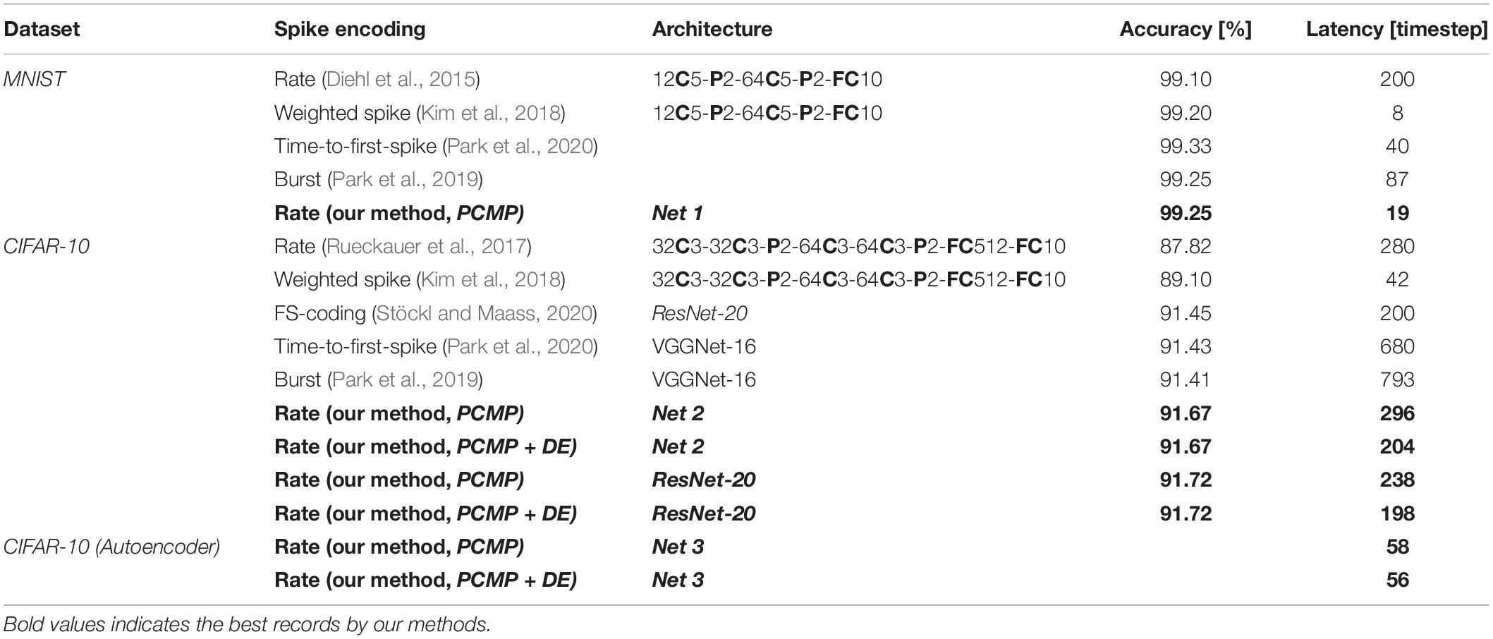
Table 3. Comparison with prior work.

Conclusion

In this work, methods to reduce the inherent latency in SNN are proposed, which is applicable at the inference stage. The membrane potential of a neuron is charged to some extent prior to inference operation, which is denoted as the pre-charged membrane potential (PCMP). Also, we introduce a deliberate delay in the output layer to discard some spikes occurring at the initial timesteps, referred as a DE. It is demonstrated through the model equations of SNNs that PCMP reduces the SNN error by inducing the earlier firing of the first spike, and DE eliminates the error spikes at the early timesteps so that low-latency SNN can be achieved. In SNN applications, such as classification and autoencoder, the proposed methods successfully reduce the latency, the combined use of PCMP and DE can help to achieve further latency reduction. Moreover, required the synaptic operations are significantly improved by using the proposed methods, which leads to energy-efficient computing.

Data Availability Statement

The original contributions presented in the study are included in the article/Supplementary Material, further inquiries can be directed to the corresponding author/s.

Author Contributions

SH, JC, M-HO, and KM: conceptualization. TJ, KP, and JY: data curation. SH: writing—original draft preparation. SH and B-GP: writing and editing. J-HL and B-GP: supervision. B-GP: project administration. All authors have read and agreed to the submitted version of the manuscript.

Funding

This work was supported by the BK21 FOUR program of the Education and Research Program for Future ICT Pioneers, Seoul National University in 2020 and in part by Institute of Information and Communications Technology Planning and Evaluation (IITP) grant funded by the Korea government (MSIT) (No. 2020-0-01294, Development of IoT based edge computing ultra-low power artificial intelligent processor).

Conflict of Interest

The authors declare that the research was conducted in the absence of any commercial or financial relationships that could be construed as a potential conflict of interest.

References

Amir, A., Taba, B., Berg, D., Melano, T., Mckinstry, J., Di Nolfo, C., et al. (2017). “A low power, fully event-based gesture recognition system,” in Proceedings of the IEEE Conference on Computer Vision and Pattern Recognition, (Piscataway, NJ: IEEE), 7243–7252.

Google Scholar

Cao, Y., Chen, Y., and Khosla, D. (2015). Spiking deep convolutional neural networks for energy-efficient object recognition. Int. J. Comp. Vis. 113, 54–66.

Google Scholar

Cardarilli, G. C., Cristini, A., Di Nunzio, L., Re, M., Salerno, M., and Susi, G. (2013). “Spiking neural networks based on LIF with latency: Simulation and synchronization effects,” in Proceedings of the 2013 Asilomar Conference on Signals, Systems and Computers, (Piscataway, NJ: IEEE), 1838–1842.

Google Scholar

Chen, C., Seff, A., Kornhauser, A., and Xiao, J. (2015). “Deepdriving: learning affordance for direct perception in autonomous driving,” in Proceedings of the IEEE International Conference on Computer Vision, (Piscataway, NJ: IEEE), 2722–2730.

Google Scholar

Diehl, P. U., Neil, D., Binas, J., Cook, M., Liu, S.-C., and Pfeiffer, M. (2015). “Fast-classifying, high-accuracy spiking deep networks through weight and threshold balancing,” in Proceedings of the Neural Networks (IJCNN), 2015 International Joint Conference on: IEEE, (Piscataway, NJ: IEEE), 1–8.

Google Scholar

Ghosh-Dastidar, S., and Adeli, H. (2009). Spiking neural networks. Int. J. Neural. Syst. 19, 295–308.

Google Scholar

Gütig, R., and Sompolinsky, H. (2006). The tempotron: a neuron that learns spike timing–based decisions. Nat. Neurosci. 9, 420–428. doi: 10.1038/nn1643

PubMed Abstract | CrossRef Full Text | Google Scholar

Han, S., Mao, H., and Dally, W. J. (2015). Deep compression: compressing deep neural networks with pruning, trained quantization and huffman coding. arXiv [preprint].

Google Scholar

He, K., Zhang, X., Ren, S., and Sun, J. (2016). “Deep residual learning for image recognition,” in Proceedings of the IEEE Conference on Computer Vision and Pattern Recognition, (Piscataway, NJ: IEEE), 770–778.

Google Scholar

Hu, Y., Tang, H., Wang, Y., and Pan, G. (2018). Spiking deep residual network. arXiv [preprint].

Google Scholar

Hubara, I., Courbariaux, M., Soudry, D., El-Yaniv, R., and Bengio, Y. (2017). Quantized neural networks: training neural networks with low precision weights and activations. J. Mach. Learn. Res. 18, 6869–6898.

Google Scholar

Hubara, I., Courbariaux, M., Soudry, D., El-Yaniv, R., and Bengio, Y. (2016). “Binarized neural networks,” in Proceedings of the Advances in Neural Information Processing Systems, (Vancouver: NIPS) 4107–4115.

Google Scholar

Hwang, S., Chang, J., Oh, M.-H., Lee, J.-H., and Park, B.-G. (2020). Impact of the sub-resting membrane potential on accurate inference in spiking neural networks. Sci. Rep. 10:3515.

Google Scholar

Iakymchuk, T., Rosado-Muñoz, A., Guerrero-Martínez, J. F., Bataller-Mompeán, M., and Francés-Víllora, J. V. (2015). Simplified spiking neural network architecture and STDP learning algorithm applied to image classification. EURASIP J. Image Video Process. 2015:4.

Google Scholar

Indiveri, G., Corradi, F., and Qiao, N. (2015). “Neuromorphic architectures for spiking deep neural networks,” in Proceedings of the 2015 IEEE International Electron Devices Meeting (IEDM), (Piscataway, NJ: IEEE).

Google Scholar

Kim, J., Kim, H., Huh, S., Lee, J., and Choi, K. (2018). Deep neural networks with weighted spikes. Neurocomputing 311, 373–386. doi: 10.1016/j.neucom.2018.05.087

CrossRef Full Text | Google Scholar

Krizhevsky, A., Sutskever, I., and Hinton, G. (2017). Imagenet classification with deep convolutional neural networks. Commun. ACM 60, 84–90. doi: 10.1145/3065386

CrossRef Full Text | Google Scholar

LeCun, Y., Bengio, Y., and Hinton, G. (2015). Deep learning. Nature 521, 436–444.

Google Scholar

Li, H., Lin, Z., Shen, X., Brandt, J., and Hua, G. (2015). “A convolutional neural network cascade for face detection,” in Proceedings of the IEEE Conference on Computer Vision and Pattern Recognition, (Piscataway, NJ: IEEE), 5325–5334.

Google Scholar

Maass, W. (1997). Networks of spiking neurons: the third generation of neural network models. Neural. Netw. 10, 1659–1671. doi: 10.1016/s0893-6080(97)00011-7

CrossRef Full Text | Google Scholar

Merolla, P. A., Arthur, J. V., Alvarez-Icaza, R., Cassidy, A. S., Sawada, J., Akopyan, F., et al. (2014). A million spiking-neuron integrated circuit with a scalable communication network and interface. Science 345, 668–673. doi: 10.1126/science.1254642

PubMed Abstract | CrossRef Full Text | Google Scholar

Neil, D., Pfeiffer, M., and Liu, S.-C. (2016). “Learning to be efficient: algorithms for training low-latency, low-compute deep spiking neural networks,” in Proceedings of the 31st Annual ACM Symposium on Applied Computing, (New York, NY: ACM), 293–298.

Google Scholar

O’Connor, P., and Welling, M. (2016). Deep spiking networks. arXiv [preprint].

Google Scholar

Park, S., Kim, S., Choe, H., and Yoon, S. (2019). “Fast and efficient information transmission with burst spikes in deep spiking neural networks,” in Proceedings of the 2019 56th ACM/IEEE Design Automation Conference (DAC), (Piscataway, NJ: IEEE), 1–6.

Google Scholar

Park, S., Kim, S., Na, B., and Yoon, S. (2020). “T2FSNN: deep spiking neural networks with time-to-first-spike coding,” in Proceedings of the 57th ACM/IEEE Design Automation Conference (DAC), (Piscataway, NJ: IEEE).

Google Scholar

Paugam-Moisy, H., and Bohte, S. (2012). Computing with Spiking Neuron Networks. Berlin: Springer.

Google Scholar

Ponulak, F., and Kasiński, A. (2010). Supervised learning in spiking neural networks with ReSuMe: sequence learning, classification, and spike shifting. Neural. Comput. 22, 467–510. doi: 10.1162/neco.2009.11-08-901

PubMed Abstract | CrossRef Full Text | Google Scholar

Ponulak, F., and Kasiński, A. (2011). Introduction to spiking neural networks: information processing, learning and applications. Acta Neurobiol. Exp. 71, 409–433.

Google Scholar

Rosenblatt, F. (1958). The perceptron: a probabilistic model for information storage and organization in the brain. Psychol. Rev. 65:386. doi: 10.1037/h0042519

PubMed Abstract | CrossRef Full Text | Google Scholar

Rueckauer, B., and Liu, S.-C. (2018). “Conversion of analog to spiking neural networks using sparse temporal coding,” in 2018 IEEE International Symposium on Circuits and Systems (ISCAS): IEEE, 1–5.

Google Scholar

Rueckauer, B., Lungu, I.-A., Hu, Y., Pfeiffer, M., and Liu, S.-C. (2017). Conversion of continuous-valued deep networks to efficient event-driven networks for image classification. Front. Neurosci. 11:682. doi: 10.3389/fnins.2017.00682

PubMed Abstract | CrossRef Full Text | Google Scholar

Rullen, R. V., and Thorpe, S. J. (2001). Rate-based coding versus temporal order coding: what the retinal ganglion cells tell the visual cortex. Neural Comput. 13, 1255–1283. doi: 10.1162/08997660152002852

PubMed Abstract | CrossRef Full Text | Google Scholar

Schmidhuber, J. (2015). Deep learning in neural networks: an overview. J. Neural Netw. 61, 85–117. doi: 10.1016/j.neunet.2014.09.003

PubMed Abstract | CrossRef Full Text | Google Scholar

Sengupta, A., Ye, Y., Wang, R., Liu, C., and Roy, K. (2019). Going deeper in spiking neural networks: VGG and residual architectures. Front. Neurosci. 13:95. doi: 10.3389/fnins.2019.00095

PubMed Abstract | CrossRef Full Text | Google Scholar

Seo, J.-S., Brezzo, B., Liu, Y., Parker, B. D., Esser, S. K., Montoye, R. K., et al. (2011). “A 45nm CMOS neuromorphic chip with a scalable architecture for learning in networks of spiking neurons,” in Proceedings of the 2011 IEEE Custom Integrated Circuits Conference (CICC), (Piscataway, NJ: IEEE), 1–4.

Google Scholar

Springenberg, J. T., Dosovitskiy, A., Brox, T., and Riedmiller, M. A. (2014). Striving for simplicity: the all convolutional net. arXiv [preprint].

Google Scholar

Stöckl, C., and Maass, W. (2020). Classifying Images with few spikes per neuron. arXiv [preprint].

Google Scholar

Stromatias, E., Neil, D., Galluppi, F., Pfeiffer, M., Liu, S.-C., and Furber, S. (2015). “Scalable energy-efficient, low-latency implementations of trained spiking deep belief networks on SpiNNaker,” in Proceedings of the 2015 International Joint Conference on Neural Networks (IJCNN), (Piscataway, NJ: IEEE), 1–8.

Google Scholar

Tavanaei, A., Ghodrati, M., Kheradpisheh, S. R., Masquelier, T., and Maida, A. (2018). Deep learning in spiking neural networks. Neural Netw. 111, 47–63. doi: 10.1016/j.neunet.2018.12.002

PubMed Abstract | CrossRef Full Text | Google Scholar

Thorpe, S., Delorme, A., and Van Rullen, R. (2001). Spike-based strategies for rapid processing. Neural Netw. 14, 715–725. doi: 10.1016/s0893-6080(01)00083-1

CrossRef Full Text | Google Scholar

Webb, B., and Scutt, T. (2000). A simple latency-dependent spiking-neuron model of cricket phonotaxis. Biol. Cybern. 82, 247–269. doi: 10.1007/s004220050024

PubMed Abstract | CrossRef Full Text | Google Scholar

Yang, T.-J., Chen, Y.-H., and Sze, V. (2017). “Designing energy-efficient convolutional neural networks using energy-aware pruning,” in Proceedings of the IEEE Conference on Computer Vision and Pattern Recognition, (Piscataway, NJ: IEEE), 5687–5695.

Google Scholar

Zenke, F., and Ganguli, S. (2018). Superspike: supervised learning in multilayer spiking neural networks. Neural Comput. 30, 1514–1541. doi: 10.1162/neco_a_01086

CrossRef Full Text | Google Scholar

Zhang, T., Zeng, Y., Zhao, D., and Shi, M. (2018). “A plasticity-centric approach to train the non-differential spiking neural networks,” in Proceedings of the Thirty-Second AAAI Conference on Artificial Intelligence, (New Orleans, LA).

Google Scholar