- School of Computer Science and Engineering, University of Electronic Science and Technology of China, Chengdu, China
Neural circuits respond to multiple sensory stimuli by firing precisely timed spikes. Inspired by this phenomenon, the spike timing-based spiking neural networks (SNNs) are proposed to process and memorize the spatiotemporal spike patterns. However, the response speed and accuracy of the existing learning algorithms of SNNs are still lacking compared to the human brain. To further improve the performance of learning precisely timed spikes, we propose a new weight updating mechanism which always adjusts the synaptic weights at the first wrong output spike time. The proposed learning algorithm can accurately adjust the synaptic weights that contribute to the membrane potential of desired and non-desired firing time. Experimental results demonstrate that the proposed algorithm shows higher accuracy, better robustness, and less computational resources compared with the remote supervised method (ReSuMe) and the spike pattern association neuron (SPAN), which are classic sequence learning algorithms. In addition, the SNN-based computational model equipped with the proposed learning method achieves better recognition results in speech recognition task compared with other bio-inspired baseline systems.
1. Introduction
For years, researchers have been exploring and trying to simulate the brain's powerful and high-speed information processing capabilities and learning mechanisms. While the traditional artificial neural networks (ANNs) have achieved outstanding performance in various application fields, they assume that sensory information is represented and transmitted via the firing rate of the neuron. Nevertheless, the rate-based coding does not seem to transmit all the information associated with the rapid processing sensory tasks, such as vision, smell, and hearing stimulus modalities (Hopfield, 1995; Gautrais and Thorpe, 1998; Cariani, 2004; Mohemmed et al., 2013). A new type of artificial neural network that is dedicated to the study of more biologically plausible neuronal models and neural networks has emerged and has been well used (Wu et al., 2018a,b), which is called spiking neural networks (SNNs). On the other hand, many recent studies have shown that spike-timing neural activities exist in several areas of the brain, such as the visual cortex (Bair and Koch, 1996), the retina (Meister, 1998; Uzzell and Chichilnisky, 2004; Gollisch and Meister, 2008), and the lateral and geniculate nucleus (Reinagel and Reid, 2000). Temporally encoded SNNs that represent information as precisely timed spikes rather than mean firing rates have also been studied extensively (Maass, 1997; Andrew, 2002; Ghosh-Dastidar and Adeli, 2009b; Nguyen et al., 2012; Wang et al., 2012). Though the powerful computing performance of SNNs has been demonstrated (Keller and Hahnloser, 2009), its practical application is still limited by its computational complexity, and the learning algorithms applicable to SNNs are also generally short of high efficiency and stability. Therefore, it is of great significance to develop new effective and robust learning algorithms to take full advantage of the powerful computing performance of SNNs.
In many cases, learning behavior is thought to be performed by utilizing the error signals, i.e., the mismatches between expected and actual spiking behaviors (Thach, 1996; Bastos et al., 2012; Keller et al., 2012; Wu et al., 2019). Supervised learning based on error signals has obtained the most documented evidence in the study of the cerebellum and cerebellar cortex of the central nervous system, although the exact mechanism still remains unclear (Ito, 2000). The aim of supervised learning is to minimize the gap between actual output and expected output, and according to the different ways of reducing the gap, the existing learning algorithms of SNNs can be divided into two categories. One is to utilize rigorous mathematical analysis to derive formulas of loss reduction, and the other is to make weight updating according to the inspiration of biological mechanisms, such as the Widrow-Hoff rule (Widrow and Lehr, 1990) and the spike-timing dependent plasticity (STDP) rule (Masquelier et al., 2009), where the synaptic strength is enhanced when the presynaptic neuron elicits spikes before the postsynaptic neuron and vice versa.
Many methods based on mathematical analysis adopt the idea of gradient descent, but they define the cost function in different ways. SpikeProp (Bohte et al., 2002) minimizes the loss defined by the distance between the true firing time and the single desired firing time using gradient descent rule, and later this algorithm was improved to emit multiple spikes (Ghosh-Dastidar and Adeli, 2009a; Xu et al., 2013a). In addition to these methods, Tempotron (Gütig and Sompolinsky, 2006), an algorithm that has been proved to be effective for binary temporal classification but unable to handle the firing of multiple spikes, and some other algorithms (Zhang et al., 2018, 2019a) define the cost function as the distance between the membrane voltage and the firing threshold. Recently, there is another thought of defining cost function of multi-spike sequences. For example, Multi-Spike Tempotron (MST) (Gütig, 2016) is designed to decrease the difference between a hypothetical threshold and the fixed threshold. MST also employs the gradient descent strategy, and in each iteration the difference between the fixed biological firing threshold and the hypothetical threshold under which neurons emit the expected amount of spikes is calculated. However, it requires multiple recursive calculations to derive the hypothetical threshold, making the learning process indirect and computationally time-consuming. TDP1 and TDP2 (Yu et al., 2018) simplify the calculation of MST to some extent, which improves the learning efficiency, but there is still the problem of seeking the hypothesis threshold through iteration.
The Remote Supervised Method (ReSuMe) (Ponulak and Kasiński, 2010) is a classic algorithm that combines the STDP and anti-STDP learning rules to modulate the synaptic weights. There are also some improved algorithms to further strengthen the learning property of the ReSuMe by integrating it with delay learning (Taherkhani et al., 2015a,b, 2018), and particle swarm optimization (PSO) algorithm (Xie et al., 2014), etc. In addition, the Spike Pattern Association Neuron (SPAN) (Mohemmed et al., 2012), Chronotron E-learning (Florian, 2012), and the Precise-Spike-Driven (PSD) (Yu et al., 2013) algorithm are in a similar vein, whereby they transform spike trains or sequences into analog signals by convolution, then apply the Widrow-Hoff rule to update weights. SPAN uses a variant metric of the van Rossum metric (van Rossum, 2001) to define the distance between the actual and desired spike sequences, while Chronotron E-learning uses the Victor and Purpura metric (Victor and Purpura, 2009). SPAN transforms all the discrete input, actual and desired output spikes to continuous signals, while only input signals are convolved in PSD. Compared with algorithms requiring convolution operation, algorithms based on the perceptron rule, such as the perceptron-based spiking neuron learning rule (PBSNLR) (Xu et al., 2013b) and its improved version (Qu et al., 2015), the normalized perceptron based learning rule (NPBLR) (Xie et al., 2017), are easier to calculate. In general, these algorithms are more biologically plausible and have lower computational complexity than the algorithms based on the gradient descent rule, but they are still not very effective and robust in the task of learning target spatiotemporal spike patterns.
Except for these algorithms, the algorithm Learning Spike Sequences with Finite Precision (FP) (Memmesheimer et al., 2014) uses the existing postsynaptic potential to adjust the synaptic weights at the first unmatched time between the actual and desired output spike trains in each trial. However, the simple and crude way of weight modification makes it use less spike information and also lack good robustness in the face of noise. Then in this paper, we propose a new efficient and robust learning algorithm. The proposed algorithm not only utilizes the first wrong spike time, but also utilizes all previous spike temporal information to calculate the weight update quantities. Simulation results demonstrate that the proposed learning rule has higher learning accuracy, efficiency, and better robustness as compared with ReSuMe and SPAN. In addition, in this paper, we also put forward a dynamic decoding strategy for precise multi-spike learning algorithms. With a combination of the proposed learning algorithm and the decoding strategy, the SNN-based computational model outperforms other bio-inspired baseline systems in a speech recognition task.
The structure of the article is as follows. In 2, after a brief introduction of the neuron model, our method is presented. In 3, we conduct some experiments to explore the performance of the method, and the simulation results are provided. The different properties of the proposed algorithm, ReSuMe and SPAN are analyzed and compared in 4. Finally, we draw the conclusion in 5.
2. Neuron Model and Learning Algorithm
In this section, we first introduce the spiking neuron model used in this article, then elaborate on the algorithm we proposed. Finally, the measurement used to evaluate the learning performance is introduced.
2.1. Neuron Model
Many spiking neuron models have been proposed over the years, among which conductance-based models can simulate biological neurons' dynamics accurately to a large extent but require considerable computational cost because of the inherent complexity of their expressions. By contrast, the current-based leaky integrate-and-fire (LIF) (Gerstner and Kistler, 2002) model can well simulate the dynamics of biological neurons with lower computation cost, which has made it a widely used model in many papers, including this one.
In the LIF model, learning neuron accumulates its membrane voltage V(t) by integrating synaptic currents from N upstream neurons, yielding
where is the firing time of the jth spike from the ith synapse and is the firing time of the jth spike generated by the learning neuron. ϑ is the firing threshold. wi represents the synaptic strength of the ith synapse, and it controls the amplitude of the postsynaptic potential induced by its spike, while the kernel K(·) controls the shape, and it is defined as
where τm and τs are the time constants of the membrane potential and the synaptic current, respectively. Vnorm is the normalization constant that stretches the peak value of K(·) to unit, and it is calculated by
with β = τm/τs. If the voltage V(t) reaches the firing threshold, it triggers a spike immediately, then this new spike causes the membrane voltage of the neuron to encounter a reset operation, which is expressed by the second term in Equation (1).
2.2. First Error Learning Algorithm
The aim of our learning algorithm is to modify the neuron's synaptic weights so that it can generate the target spike sequence corresponding to the given input spike pattern. Most existing algorithms train the neuron to fire spikes directly toward the desired times, but here we set a tolerance window with a small width ε (less than the distance between any two desired spike times) at each desired time, and by training the neuron to emit a spike within the corresponding tolerance window in chronological order, the requirement of firing target spike sequence is finally achieved. Accordingly, we present our learning method taking advantage of the idea of running synaptic modification rules only at the first wrong spike time in each trial in Memmesheimer et al. (2014).
There are different types of wrong spike times, but in general they all fall into one of the three categories and are shown in Figure 1:
• If there is a spike fired outside all tolerable windows, this spike time is a wrong spike time of type a;
• If there are two spikes generated within a same window, the second spike time is a wrong spike time of type b;
• If there is no spike within the desired tolerable window, the desired spike time is a wrong spike time of type c.
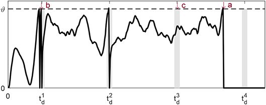
Figure 1. Three error types: undesired spike outside the tolerable window (a), undesired spike inside the tolerable window (b) and missed spike within the tolerable window (c). The gray vertical bars near the desired spike times are the respective tolerable windows.
Following the idea of running synaptic modification rules only at the first wrong spike time in each trial, the proposed First Error Learning rule (FE-Learn) calculates weight adjustment in a new way that utilizes more temporal information between the input and output spike trains. Based on the different error types, the proposed method employs two weight updating processes. The cost function is defined as
where terr is the first wrong spike time and the ± sign corresponds to weight increment and decrement, respectively.
2.2.1. Weight Increment at Desired Output Spike Times
In terms of error type c, a spike is supposed to be emitted within the tolerable window of a desired output spike time , while it is not, so terr is equal to . Then, we apply the gradient descent method to stretch the membrane potential at time terr to the threshold ϑ.
In gradient-based learning, the weight modification Δwi is proportional to the negative of the derivative of the cost function with respect to wi:
where λ1 > 0 is the learning rate that defines the size of the weight increment. From Equation (1), the membrane potential V(terr) not only receives the direct influence of the synaptic weights, but also the indirect influence of them, which is transmitted by the previous output spike times . The derivative term in Equation (5) is hence given by
From Equation (1), the first term of Equation (6) can be expressed as
and the partial derivative in the second term is
while for the derivative , applying the chain rule, we can get
in order to save the computation cost, we eliminate the iterative computation term in Equation (9). Following the linear assumption of threshold crossing in Bohte et al. (2002), Ghosh-Dastidar and Adeli (2009a), and Yu et al. (2018), the neuron's membrane potential is thought to increase linearly in the infinitesimal time step before the firing time. Hence, there is
where
and can be solved by Equation (7), and with can be solved by Equation (8).
Note that each actual output spike time before the terr is within the tolerable window of the corresponding desired spike time , and there is usually a slight deviation between and . So the weight modification strategy based on Equation (6) may exacerbate this deviation after multiple updates, resulting in more unnecessary adjustments. In order to address this, in the actual weight adjustment, we substitute for in Equation (6) through Equation (11) and give a scaling factor Sr (> 0) to the second term of Equation (6) to control the weight updating at (< terr) not excessively (the detailed analysis is presented in 4), which is proven to be meaningful and vital by experiments.
2.2.2. Weight Decrement at Undesired Output Spike Times
When there is a spike fired outside the tolerable window (error type a) or there is more than one spike fired inside the same tolerable window (error type b), the contributory synaptic weights should be weakened to prevent the extra spike. Instead of utilizing all the past firing spikes (actual or desired) like the case of weight increment, for error types a and b, synaptic weight decrement depends only on the error time terr, i.e., the scaling rate Sr is set to zero. As a result, the second term in Equation (6) is removed, and the updating rule at undesired output spikes is defined as
where λ2 > 0 is the learning rate which defines the size of the weight decrement. ∂V(terr)/∂wi is solved by Equation (7).
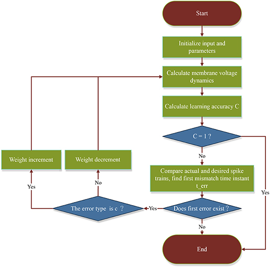
The intention of removing the second term in Equation (6) is to avoid disturbing the properly emitted output spikes before terr. How this affects the previously emitted spikes is explained in 4. To better illustrate the process of the proposed FE-Learn algorithm, we give a flowchart in Figure 2.
2.3. Metric of Learning Performance
The correlation-based metric C defined in Schreiber et al. (2003) is adopted in the next experiments to evaluate the learning performance of the learning algorithm, and it was also used in Ponulak and Kasiński (2010) and Taherkhani et al. (2015a). C(0 < C < 1) represents the similarity degree of two vectors, and the larger the value of C, the higher the similarity between the two vectors. The metric is defined in the following equation:
where υo and υd are vectors which are the convolution (in discrete time) of actual and desired output spike trains by a symmetric Gaussian filter given as f(t, σ) = exp(−t2/2σ2), respectively. The parameter σ determining the width of the filter is set to 2 in this article. And υd · υo represents the dot product of the two vectors, while |υd| and |υo| are the Euclidean norms of them, respectively.
3. Simulation results
Next, we conduct extensive experiments to explore the influence of different parameters with different values on the learning performance of the FE-Learn. Moreover, the robustness in the face of noise of different intensities is tested, and finally, FE-Learn is applied to a practical speech recognition task.
3.1. Performance Evaluation of FE-Learn
The effects of several important parameters on learning performance are investigated in this section, including the time duration of spike trains, the number of synaptic inputs, and the firing rates of input and output spike trains. We compared the FE-Learn against ReSuMe and SPAN. In these simulations, the time constant of the membrane potential and the synaptic currents, τm and τs, are set to 10 and 2.5 ms, respectively. And the firing threshold and the time step are set to 1 mV and 1 ms, respectively. The synaptic weights are randomly initialized by the Gaussian distribution N(0.01, 0.01). Twenty trials with different input and desired output pairs are conducted for each experiment.
3.1.1. Effect of the Time Duration
In this section, the learning neuron has 400 synaptic afferents. The aim is to train the neuron to reproduce a desired spike train with a time duration of 200 ~ 3,000 ms and the length of the interval is 200 ms. Before each training trial, the desired output is a spike train with a firing rate of 100 Hz, and input spike trains with a firing rate of 10 Hz are generated according to the homogeneous Poisson processes. During each training, the maximum value of C and the running time required to reach it are recorded. After 20 training trials, the average values of all maximum C and corresponding running times are reported.
Figure 3A shows the variation trend in learning accuracies of FE-Learn, SPAN, and ReSuMe. The learning accuracies of the three algorithms can reach one when the time duration of spike trains varies from 200 to 600 ms, but when the time duration exceeds 800 ms, the learning accuracies of SPAN and ReSuMe start to decline, and the learning times increase gradually. Meanwhile, the learning accuracy of FE-Learn is limited by the width of the tolerable window ε, so it can keep constant at 1 when ε = 1, C ≈ 0.96 when ε = 3 and C ≈ 0.89 when ε = 5, and the learning accuracy drops significantly when the width of the tolerable window changes. Under the same width of the tolerable window, the learning time increases with the increase of spike train length. The general trend is that FE-Learn can obtain higher learning accuracy than SPAN and ReSuMe with less time.
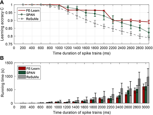
Figure 3. Effect of the time duration of spike trains on learning performance. When the time duration of spike trains is in [200, 1,000], [1,200, 2,000], [2,200, 3,000] ms, the corresponding width of the tolerable window is 1, 3, and 5 ms, respectively. Learning accuracy comparison of FE-Learn, SPAN, and ReSuMe under different time duration of spike trains (A), running time comparison of FE-Learn, SPAN, and ReSuMe under different time duration of spike trains (B).
3.1.2. Effect of the Number of the Synaptic Inputs
The effect of the number of the synaptic inputs is investigated in this section, and it varies from 100 to 500 with an interval of 50. The time duration of the spike trains is set to 800 ms. The desired output spike train with a firing rate of 100 Hz and input spike train with a firing rate of 10 Hz are generated according to the homogeneous Poisson processes at the beginning of each training trial.
Figure 4 shows the experimental results. As shown in Figure 4A, a small number of synaptic inputs lead to a low learning accuracy for both SPAN and ReSuMe—for instance, the learning accuracy of SPAN is only 0.81 and for ReSuMe it is 0.79—when the neuron is trained with only 100 synaptic inputs, but SPAN takes a very short time, and although FE-Learn with ε = 5 takes more time, it can achieve higher accuracy. When the number of synaptic inputs is greater than or equal to 300, the width of the tolerable window of FE-Learn is set to 1 ms. Then, the learning accuracy of it can reach 1, while the learning accuracies of SPAN and ReSuMe slowly increase to 1 with the increase of the number of synaptic inputs. Additionally, under the same width of the tolerable window, the learning time of FE-Learn can decrease with the increase of the number of the synaptic inputs. In short, FE-Learn performs better than ReSuMe both in terms of accuracy and running time, and obtains higher accuracy than SPAN with comparable time.
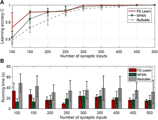
Figure 4. Effect of the number of the synaptic inputs on learning performance. When the synaptic input is in 100, [150, 250], [300, 500], the corresponding width of the tolerable window is 5, 3, and 1, respectively. Learning accuracy comparison of FE-Learn, SPAN, and ReSuMe with different number of the synaptic inputs (A), running time comparison of FE-Learn, SPAN, and ReSuMe with different number of the synaptic inputs (B).
3.1.3. Effect of the Firing Rate
The effect of the firing rate of the spike trains is evaluated in the following experiments. For the input spike trains, the firing rates (rin) are varied from 6 to 18 Hz with an interval of 4 Hz, while for the desired output spike trains the firing rates (rout) vary from 20 to 160 Hz with an interval of 20 Hz. The time duration of the spike trains is 800 ms and the amount of the synaptic inputs is set to 400. In each trial, the learning continues until the algorithm converges and the averages of the maximum obtained C from 20 trials are reported in Figure 5.
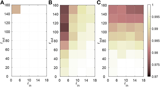
Figure 5. Effect of the firing rate of the spike trains on learning performance of FE-Learn (A), SPAN (B), and ReSuMe (C). All parameters except the firing rates of input spike trains rin and the desired output spike trains rout are fixed. The width of the tolerable window ε is set to 1.
From Figure 5A, the learning accuracy of FE-Learn can achieve 1 except when the firing rates of the input spike train and the desired output spike trains are 6 and 160 Hz, respectively, but even in this worst case, the accuracy still reaches 0.986. However, the performances of SPAN and ReSuMe become worse with the decrease of rin and the increase of rout, and their lowest accuracies are about 0.97, as shown in Figure 5B.
3.2. Robustness to Noise
In this section, the robustness of the neuron trained by FE-Learn and ReSuMe is investigated. The neuron has 400 synaptic inputs. The time duration of the input and expected spike trains is set as 500 ms, both of which are Poisson spike trains, and the firing rates of them are 10 and 100 Hz, respectively. After deterministic training, the response reliability of the neuron is considered in the case of adding background noise on the membrane potential and adding jittering noise on the input pattern.
3.2.1. Robustness to Background Noise on the Membrane Potential
After training, the membrane potential of the trained neuron is affected by background Gaussian white noise with mean 0 and variance σb ∈ [0.03, 0.33] mV in this case. The variance interval is 0.03 mV, and for every value of σb, 20 independent experiments are conducted. The metric C is still used to measure the similarity of the actual output and desired output.
As shown in Figure 6, the learning accuracies of the three algorithms decrease with the increase of noise intensity. However, the correlation metric C achieved by the neuron trained by FE-Learn is consistently higher than that of SPAN and ReSuMe, confirming that the neuron trained by FE-Learn is more robust when encountering background noise.
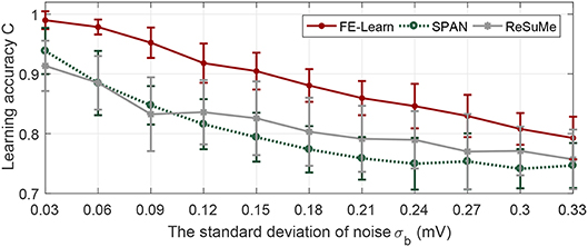
Figure 6. Antinoise capability of FE-Learn, SPAN, and ReSuMe against background voltage noise. The width of the tolerable window ε is set to 1.
3.2.2. Robustness to Jittering Noise on the Input Pattern
In this case, a Gaussian jitter with mean 0 and variance σj ∈ [0.2, 2] ms is added to each input spike after deterministic training. In addition, every spike of the noisy input pattern may be randomly deleted with a probability of 0.05 while some new spikes may be randomly added into the noisy input pattern, which are generated by a 1 Hz homogeneous Poisson process. Just as before, the correlation measure C of the distance between the actual and the desired output spike sequences is calculated.
As can be seen from Figure 7, with the increase of the noise intensity, the correlation between the actual and the desired output spike trains shows a gradual downward trend, but for FE-Learn, it stays about 0.05 and 0.1 higher than that of SPAN and ReSuMe, respectively. Unlike before, SPAN performs better than ReSuMe when exposed to jitter noise. However, neurons trained by the FE-Learn have better anti-noise performance against jitter noise than either of them.
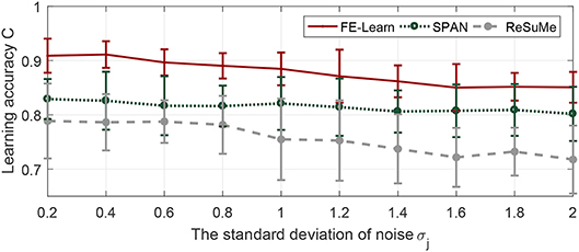
Figure 7. Antinoise capability of FE-Learn, SPAN, and ReSuMe against jittering noise. The width of the tolerable window ε is set to 1.
3.3. Effect of Learning Parameters
The width of the tolerance window ε and the scaling rate Sr are two important parameters of FE-Learn. We conduct experiments to explore the influence of them on learning efficiency and robustness of FE-Learn. Then we give a spatiotemporal spike pattern recognition experiment, and show the effect of ε on the testing performance.
3.3.1. Effect on Efficiency
In this section, the learning neuron has 400 synaptic afferents, and the time duration is 800 ms. Input pattern and target pattern are generated as in the previous experiments with a firing rate of 10 and 400, respectively. The scaling rate varies from 0 to 2 with an interval of 0.2, and the width of the tolerance window has four different values, 1, 3, 5, and 7 (under the condition that time step equals one, width equal to 2 is actually the same as width equal to 1, so there is no need to explore the situation of 2, 4, and 6). For each pair of ε and Sr, the learning continues until the algorithm converges and the average of the maximum obtained C from 20 trials are reported in Figure 8.
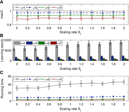
Figure 8. Effect of tolerance window width and scaling rate on learning efficiency. The evaluation index includes learning accuracy (A), the number of epochs (B), and the running time (C).
Tolerance window width determines the learning accuracy of convergence, and Figure 8A shows this obviously, and it also shows that no matter what the scaling rate is, the algorithm will eventually converge to the accuracy limited by the corresponding window width. From Figures 8B,C, we can see that, only when the tolerance window width is 1, the time of convergence increases as the scaling rate increases, and is always much higher than other cases, i.e., when the width is greater than 1, the scaling rate has little impact on the convergence speed, and the convergence time is always very small.
3.3.2. Effect on Robustness
The experiment settings are the same as last section, except that the time duration is changed to 500 ms. We add background noise and jittering noise to the network after each training trial.
As seen in Figure 9, whether for background noise or jittering noise, the smaller the tolerance window width, the stronger the noise resistance. From Figure 9A, the antinoise capability against background noise becomes stronger with the increase of scaling rate, but from Figure 9B, the antinoise capability against jittering noise does not change obviously with the change of scaling rate.
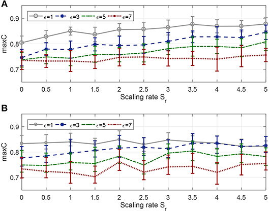
Figure 9. Effect of tolerance window width and scaling rate on robustness. (A) Antinoise capability against background noise with standard deviation σb = 0.2. (B) Antinoise capability against jittering noise with standard deviation σj = 1.
Combined with Figures 8, 9, when the window width is greater than 1, FE-Learn can converge rapidly and the convergence speed is not sensitive to the scaling rate, but increasing it can improve the antinoise performance to background noise. When the width is 1, the convergence speed of the algorithm is very slow, and the smaller the scaling rate is, the faster the convergence speed is, but the worse the antinoise performance to background noise is.
3.3.3. Effect of the Width of Tolerance Window on Overfitting
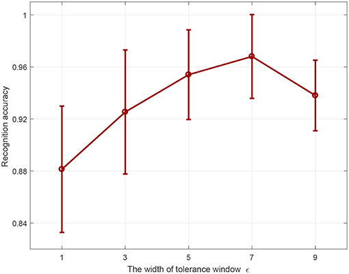
In this section, we conduct experiments to investigate the effect of the width of tolerance window on overfitting. Three different spatiotemporal spike patterns are randomly generated with 400 synaptic afferents, all of which are triggered at 5 Hz. The time duration of each spatiotemporal spike pattern is 200 ms. For each spike pattern, 25 samples are generated for training by adding a jitter noise drawn from a Gaussian distribution with a standard deviation of 3 ms, resulting in a training set with 3 × 25 samples. The test set is obtained in the same way. The learning neuron is trained to emit the corresponding desired output spike trains ([5:15:170], [15:15:180], [25:15:190]) in response to the three kinds of spike patterns. When the actual output spike train is most similar to the desired output spike train of a category, then the input pattern is classified into that category. For each ε, the average recognition accuracy on the test set from 20 trials is reported in Figure 10.
As shown in Figure 10, when ε is less than or equal to 7 ms, the classification accuracy on the test set increases with the increase of window width. This is because a smaller window means more rigorous learning on the training set, which will lead to overfitting and reduce the generalization on the test set. For example, when the window width is 7 ms, the mean recognition accuracy on the test set is 96%. However, when the window width is 1 ms, the accuracy is only about 88%. On the other hand, an overly large window will make the training insufficient, thus reducing the recognition accuracy. For instance, the recognition accuracy decreases to 93.80% when the window width is 9 ms. In a nutshell, a relatively large ε generalizes better, and the recognition accuracy on the unseen data is higher.
3.4. Classification Task
3.4.1. Spatiotemporal Spike Pattern Classification
In this experiment, we investigate the ability of the proposed FE-Learn in classifying spatiotemporal patterns. The setup for the experiment is the same as in section 3.3.3. The aim of the task is to classify three different spatiotemporal spike patterns. Both the training set and test set contain 3 × 25 samples. For each algorithm, after 300 learning epochs on the training set, the classification performance on the training set and test set is tested. The results are shown in Figure 11.
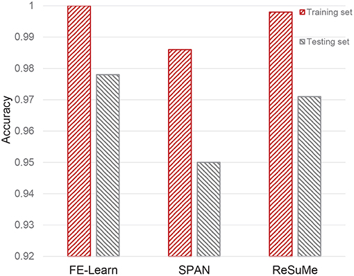
Figure 11. Classification capability of FE-Learn, SPAN, and ReSuMe on spatiotemporal spike patterns.
As can be seen from Figure 11, the classification accuracies of FE-learn, SPAN, and ReSuMe on the training set are 1, 0.986, and 0.998 while those on the test set are 0.978, 0.95, and 0.971, respectively. FE-Learn achieves better performance in both the training set and test set. On the other hand, from the respective differences between the training accuracy and the testing accuracy (0.022 for FE-Learn, 0.036 for SPAN, 0.027 for ReSuMe), FE-Learn has a better generalization ability.
3.4.2. Speech Classification
SNNs have great advantages in handling temporally rich signals since they can transform the spatiotemporal information into desired output spike patterns, which means that SNNs are well-suited for realistic tasks such as motion and speech recognition. In order to verify the capability of FE-Learn, the spiking neurons trained by the algorithm are used to conduct a spoken digit classification task. In this work, we investigate the TIDIGITS corpus (Leonard and Doddington, 1993), one of the most commonly used data sets in benchmarking speech recognition algorithms. The utterances of this data set were collected from speakers who come from 22 different dialectical regions and are digit sequences, containing 11 words: “zero,” “one,” ··· , “nine,” and “oh.”
In this case, the threshold encoding mechanism (Gütig et al., 2009) is adopted to encode the speech data into spike patterns, and the encoding mode is the same as that in Zhang et al. (2019b). Firstly, a Constant-Q Transform (CQT) cochlear filter bank (Pan et al., 2018) is used to filter the original speech waveform to get a spectrogram. Then, the spectrogram is divided into multiple frequency bins. For each bin, a cochlear filter of the corresponding frequency is used to filter it into a series of spikes by recording events that cross thresholds up and down. Finally, the spikes filtered by all cochlear filters are vertically integrated to obtain a complete input spike pattern. Referring to the visualization processing tool of auditory information provided in Dominguez-Morales et al. (2016), a visual representation of this process is given in Figure 12. In the experiment, the training set and test set include 2,464 and 2,486 speech spike patterns, respectively.
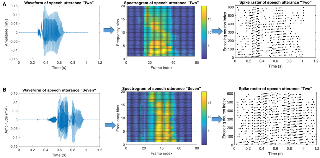
Figure 12. Threshold coding mechanism of speech data. (A) The Encoding process of a speech utterance “Two.” (B) The Encoding process of a speech utterance “Seven.” The left column shows the original speech waveforms, the middle column shows corresponding spectrograms and the right column shows the final encoded spike pattern.
The computational model used here is shown in Figure 13. There are eleven groups of output neuron in the classification layer, and each group contains ten neurons, which correspond to the same category. The goal of this experiment is to train the target group of neurons to emit a desired spike train when receiving the input patterns of the corresponding category, and to remain silent otherwise. However, it is not clear how to determine the target output spike train corresponding to each category as each speech digit category contains many different sub-patterns and the differences between these sub-patterns make a fixed desired output spike train impractical. To resolve this problem, a strategy for dynamically determining the target spike train is proposed as follows.
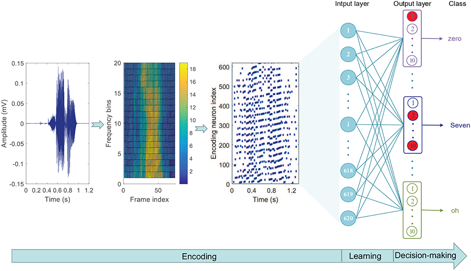
Figure 13. Network architecture of speech classification. The three diagrams on the left show the encoding process of the speech data and the network structure is on the right. The input layer contains 620 neurons and the output layer contains 11 groups of neuron (mullion), corresponding to 11 output categories, and each group is composed of ten neurons. Among the ten output neurons with the same serial number in these 11 groups, the one that emits the most spikes is the “activated” neuron (red circle). The output category belongs to the group with the largest number of “activated” neurons.
When entering a training input pattern, we record the membrane voltage traces of target neurons and non-target neurons. The desired spike trains Td and the first wrong time terr are defined as follows.
1. For the non-target neurons: Td = ∅.
• If no spike is generated, no learning is required.
• If the actual output spike trains To ≠ ∅, then the first wrong spike time terr is the first actual output spike time.
2. For the non-target neurons: Td is dynamically determined, and suppose tmax is the time instant when the maximum membrane voltage Vmax under the threshold is reached. ϑe (< ϑ) is a pre-defined encoding threshold.
• If no spike is generated, Td = {tmax}, then obviously, terr = tmax.
• If the actual output spike trains To ≠ ∅ and Vmax is above the pre-defined encoding threshold ϑe, then Td = To ∪ {tmax}, terr = tmax.
• If the actual output spike trains To ≠ ∅ and Vmax is below the pre-defined encoding threshold ϑe, then Td = To and no learning is required.
According to the defined Td and terr, the corresponding weight updating formula is called for learning. During the test, the output category belongs to the group with the largest number of activated neurons (red neuron shown in the output layer in Figure 13). Moreover, the training strategy with margins in Gütig (2016) is applied in this work. We also test the performance of ReSuMe and SPAN on this task with the same network configuration, encoding method, and training strategy as FE-Learn.
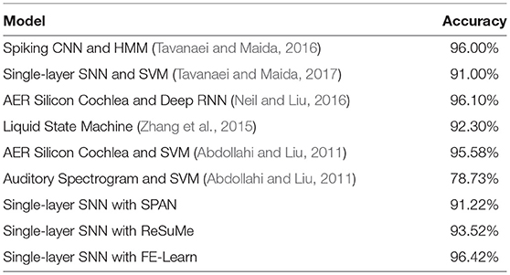
As shown in Table 1, the spiking convolutional neural network (Tavanaei and Maida, 2016) and the deep recurrent network (Neil and Liu, 2016) perform well in this speech recognition task, and they can obtain an accuracy of 96 and 96.1%, respectively. However, compared with their complex network structures, the computational model we used here is very simple while the accuracy of our method is higher than others. As shown in Table 1, the single layer spiking neural network with the proposed FE-Learn algorithm obtains an accuracy of 96.42%, which is superior to other biologically motivated baselines, as well as ReSuMe and SPAN with the same network structure, encoding scheme, and training strategy. The excellent performance of FE-Learn shows its great potential in practical application.
Additionally, in order to investigate the performance of FE-Learn in more complex cases, we also conduct speech classification experiments of the three algorithms with different input noise intensities. The standard deviation of jitter noise added to the input spike pattern increases from 0.5 to 5 ms with an interval of 0.5 ms. As shown in Figure 14, the classification accuracy of the proposed FE-Learn is 94.69% even when the noise intensity is 5 ms, which is much higher than ReSuMe and SPAN with the same noise level. Therefore, the robustness of the FE-Learn is better than ReSuMe and SPAN in practical application.
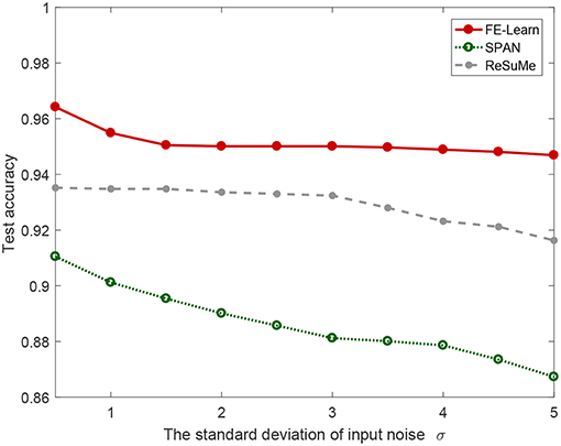
Figure 14. Speech recognition performance of FE-learn, SPAN, and ReSuMe in the test set in the face of input noise.
4. Discussion
In this section, we first analyze the difference between the three algorithms and explain the role of the parameter Sr through a concrete example. Then we figure out the reasons that contribute to FE-Learn's better performance over ReSuMe and SPAN in accuracy, computation time, and generalization.
The membrane potential curves before and after a single weight updating have been shown in Figures 15A,C, respectively. In Figure 15B, the synaptic learning curves depict the spike-timing dependence of weight adjustment at time terr. ReSuMe has an exponential learning curve (the gray dashed line), which means that the closer the input spike time is to terr, the larger the synaptic weight update is. However, due to the existence of the time constants of the membrane voltage and synaptic current, the input spike closest to terr does not make the largest contribution to the membrane voltage at terr, so the learning of ReSuMe does not serve the aim very well. As for SPAN, we depict its spike-timing dependence curve (green dotted line) of weight adjustment with α-kernel in Mohemmed et al. (2012) at time terr. From Figure 15A, each actual output spike time before the terr is within the tolerable window of the corresponding desired spike time. Accordingly, the convolution of the error is very small, resulting in very little weight change at terr. The shape of the learning curve is determined by the convolution kernel, and the inconsistency between the convolution kernel and the current kernel of the neuron model can also lead to mismatching between the weight change of the synaptic and its potential contribution.
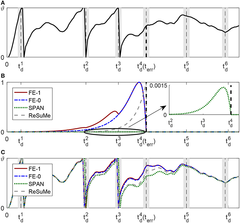
Figure 15. Comparison between FF-learn, SPAN, and ReSuMe for one weight updating. The neuron has been trained to elicit the first three spikes in corresponding tolerable windows, which are represented by the gray shadow region, the desired spike times are located at the middle of the windows. The black vertical dashed lines represent the first wrong time terr. (A) Membrane dynamics of the neuron before this learning. (B) Synaptic learning curves of FE-Learn with scaling rate Sr = 1 (red solid line) FE-Learn with scaling rate Sr = 0 (blue dotted line), SPAN (green dotted line), and ReSuMe (gray dashed line). (C) Membrane dynamics of the neuron after one learning using different rules.
As we already know, FE-learn with Sr = 1 utilizes all the spike times before terr to calculate weight increment, so the learning curve of it has multiple crests compared with that of FE-learn with Sr = 0 which has one crest. It means that the former would promote the synaptic weights whose input spikes happened before with a larger amount, but for those spikes fired between and , the weight updates are the same (the red solid line and the blue dashed line coincide). As shown in Figure 15C, the membrane potential at is successfully raised in all cases, and the spike times before are pushed forward a little bit. But for FE-learn with Sr = 1, this is more obvious than others because of the greater weight updates and thus the greater voltages at these times, which means that it is more robust to noise disturbance. However, an overly strong weight update may cause the previous output spikes to be removed from the corresponding tolerable windows, so the appropriate strength of weight adjustment at previous desired spike times which is controlled by the scaling factor Sr is crucial. As for the case of weight decrement, we only want to reduce the membrane voltage at terr, but do not want the previously correctly emitted spikes to be affected, so setting Sr to zero is reasonable.
As shown in the experimental results, FE-Learn achieves a higher learning accuracy with less training time and has a better generalization. First of all, the reason for the high accuracy of our method is that our method follows the BPBA (Bigger PSP, Bigger Adjustment) (Xu et al., 2013a) principle to effectively overcome learning interference among multiple desired spikes, while the weight update rules in ReSuMe and SPAN cannot be combined with the BPBA principle. Besides, to improve the efficiency of the program, we have calculated and stored the PSPs (Postsynaptic potentials) of every time step before training. For example, when the time duration is T, the time step is dt and the number of the synaptic inputs is N, storing the calculated PSPs requires N · T/dt storage units. For the three algorithms, the calculation of the neuron dynamics and weight adjustments are all based on the stored PSPs, and the additional memory costs required by them are very small, implying that they have a similar memory overhead. On the other hand, in each training epoch, ReSuMe makes multiple weight adjustments at each desired and actual firing time, while SPAN changes weight at each time step. However, FE-Learn only makes a weight adjustment once at terr in one epoch, and the membrane potential after terr does not need to be calculated in our experiments. This is the reason that FE-Learn requires less computation time. Finally, as the constraint on the tolerable window for spiking loosens, the generalization ability of proposed FE-learn learning is much better than others. This is the reason for the better results in Figure 11.
5. Conclusion
The proposed FE-Learn is designed for identifying spatiotemporal spike patterns, i.e., the neuron is trained to output the specific spike sequence for the given input spike pattern. FE-Learn adjusts the synaptic weights at the first wrong output spike time, and only when the trained neuron correctly fires the first spike at the desired time does FE-Learn begin to focus on adjusting the weights to fire the second desired spike. The adjustment of the synaptic weight is proportional to the derivative of the membrane voltage of the first wrong time with respect to the synapse. These three error types described above actually belong to two types: one is at the desired spike time, the other is at the actual spike time. They correspond to the two opposite cases of increasing and decreasing synaptic weights. For the first case, the desired spike times before the wrong spike time are also used to calculate the derivative, but for the second case, only the wrong spike time is used.
Although the proposed FE-Learn has reliable performance in the experiments, the inherent properties of this algorithm make it converge to the narrow window of the desired spike times, and it is difficult to emit a precisely timed spike. Hence we will explore how to balance the width of the window (accuracy) and the learning speed in the next work. Furthermore, extending FE-Learn to multi-layer deep spiking neural networks is another interesting future direction to explore.
Data Availability
The datasets analyzed for this study can be found in the TIDIGITS speech corpus https://catalog.ldc.upenn.edu/LDC93S10.
Author Contributions
XL performed the experiments and writing. XL, HQ, YC, and YZ contributed to the experiment's design and interpretation of the results.
Funding
This work was supported in part by the National Science Foundation of China under Grant 61573081 and Grant 61806040, and in part by the Foundation for Youth Science and Technology Innovation Research Team of Sichuan Province under Grant 2016TD0018.
Conflict of Interest Statement
The authors declare that the research was conducted in the absence of any commercial or financial relationships that could be construed as a potential conflict of interest.
References
Abdollahi, M., and Liu, S.-C. (2011). “Speaker-independent isolated digit recognition using an aer silicon cochlea[c],” in Biomedical Circuits & Systems Conference IEEE (La Jolla, CA).
Andrew, A. M. (2002). Spiking neuron models: single neurons, populations, plasticity. Kybernetes 4, 277C280. doi: 10.1108/k.2003.06732gae.003
Bair, W., and Koch, C. (1996). Temporal precision of spike trains in extrastriate cortex of the behaving macaque monkey. Neural Comput. 8:1185. doi: 10.1162/neco.1996.8.6.1185
Bastos, A. M., Usrey, W. M., Adams, R. A., Mangun, G. R., Fries, P., and Friston, K. J. (2012). Canonical microcircuits for predictive coding. Neuron 76, 695–711. doi: 10.1016/j.neuron.2012.10.038
Bohte, S. M., Kok, J. N., and La Poutre, H. (2002). Error-backpropagation in temporally encoded networks of spiking neurons. Neurocomputing 48, 17–37. doi: 10.1016/S0925-2312(01)00658-0
Cariani, P. A. (2004). Temporal codes and computations for sensory representation and scene analysis. IEEE Trans. Neural Netw. 15, 1100–1111. doi: 10.1109/TNN.2004.833305
Dominguez-Morales, J. P., Jimenez-Fernandez, A., Dominguez-Morales, M., and Jimenez-Moreno, G. (2016). Navis: neuromorphic auditory visualizer tool. Neurocomputing 237, 418–422. doi: 10.1016/j.neucom.2016.12.046
Florian, R. A. V. (2012). The chronotron: a neuron that learns to fire temporally precise spike patterns. PLoS ONE 7:e40233. doi: 10.1371/journal.pone.0040233
Gautrais, J., and Thorpe, S. (1998). Rate coding versus temporal order coding: a theoretical approach. Biosystems 48, 57–65. doi: 10.1016/S0303-2647(98)00050-1
Gerstner, W., and Kistler, W. M. (2002). Spiking Neuron Models. Cambridge: Cambridge University Press.
Ghosh-Dastidar, S., and Adeli, H. (2009a). A new supervised learning algorithm for multiple spiking neural networks with application in epilepsy and seizure detection. Neural Netw. 22, 1419–1431. doi: 10.1017/CBO9780511815706
Ghosh-Dastidar, S., and Adeli, H. (2009b). Spiking neural networks. Int. J. Neural Syst. 19, 295–308. doi: 10.1142/S0129065709002002
Gollisch, T., and Meister, M. (2008). Rapid neural coding in the retina with relative spike latencies. Science 319, 1108–1111. doi: 10.1126/science.1149639
Gütig, R. (2016). Spiking neurons can discover predictive features by aggregate-label learning. Science 351:aab4113. doi: 10.1126/science.aab4113
Gütig, R., and Sompolinsky, H. (2006). The tempotron: a neuron that learns spike timing-based decisions. Nat. Neurosci. 9, 420–428. doi: 10.1038/nn1643
Gütig, R., Sompolinsky, H., and Deweese, M. R. (2009). Time-warp-invariant neuronal processing. PLoS Biol. 7:e1000141. doi: 10.1371/journal.pbio.1000141
Hopfield, J. J. (1995). Pattern recognition computation using action potential timing for stimulus representation. Nature 376, 33–36. doi: 10.1038/376033a0
Ito, M. (2000). Mechanisms of motor learning in the cerebellum. Brain Res. 886, 237–245. doi: 10.1016/S0006-8993(00)03142-5
Keller, G. B., Bonhoeffer, T., and Hübener, M. (2012). Sensorimotor mismatch signals in primary visual cortex of the behaving mouse. Neuron 74, 809–815. doi: 10.1016/j.neuron.2012.03.040
Keller, G. B., and Hahnloser, R. H. (2009). Neural processing of auditory feedback during vocal practice in a songbird. Nature 457, 187–90. doi: 10.1038/nature07467
Leonard, R. G., and Doddington, G. (1993). Tidigits Speech Corpus. Philadelphia, PA: Linguistic Data Consortium.
Maass, W. (1997). Network of spiking neurons: the third generation of neural network models. Trans. Soc. Comput. Simul. Int. 14, 1659–1671. doi: 10.1016/S0893-6080(97)00011-7
Masquelier, T., Guyonneau, R., and Thorpe, S. J. (2009). Competitive stdp-based spike pattern learning. Neural Comput. 21:1259. doi: 10.1162/neco.2008.06-08-804
Meister, M. (1998). “Refractoriness and neural precision,” in Conference on Advances in Neural Information Processing Systems (Denver, CO), 110–116.
Memmesheimer, R. M., Ran, R., ölveczky, B., and Sompolinsky, H. (2014). Learning precisely timed spikes. Neuron 82, 925–938. doi: 10.1016/j.neuron.2014.03.026
Mohemmed, A., Schliebs, S., Matsuda, S., and Kasabov, N. (2012). Span: spike pattern association neuron for learning spatio-temporal spike patterns. Int. J. Neural Syst. 22:1250012. doi: 10.1142/S0129065712500128
Mohemmed, A., Schliebs, S., Matsuda, S., and Kasabov, N. (2013). Training spiking neural networks to associate spatio-temporal inputcoutput spike patterns. Neurocomputing 107, 3–10. doi: 10.1016/j.neucom.2012.08.034
Neil, D., and Liu, S. C. (2016). “Effective sensor fusion with event-based sensors and deep network architectures,” in IEEE International Symposium on Circuits and Systems (Montréal, QC).
Nguyen, V. A., Starzyk, J. A., Goh, W. B., and Jachyra, D. (2012). Neural network structure for spatio-temporal long-term memory. IEEE Trans. Neural Netw. Learn. Syst. 23, 971–983. doi: 10.1109/TNNLS.2012.2191419
Pan, Z., Li, H., Wu, J., and Chua, Y. (2018). “An event-based cochlear filter temporal encoding scheme for speech signals,” in 2018 International Joint Conference on Neural Networks(IJCNN) (Rio de Janeiro), 1–8.
Ponulak, F., and Kasiński, A. (2010). Supervised learning in spiking neural networks with resume: sequence learning, classification, and spike shifting. Neural Comput. 22, 467–510. doi: 10.1162/neco.2009.11-08-901
Qu, H., Xie, X., Liu, Y., Zhang, M., and Li, L. (2015). Improved perception-based spiking neuron learning rule for real-time user authentication. Neurocomputing 151, 310–318. doi: 10.1016/j.neucom.2014.09.034
Reinagel, P., and Reid, R. C. (2000). Temporal coding of visual information in the thalamus. J. Neurosci. 20:5392. doi: 10.1523/JNEUROSCI.20-14-05392.2000
Schreiber, S., Fellous, J. M., Whitmer, D., Tiesinga, P., and Sejnowski, T. J. (2003). A new correlation-based measure of spike timing reliability. Neurocomputing 52, 925–931. doi: 10.1016/S0925-2312(02)00838-X
Taherkhani, A., Belatreche, A., Li, Y., and Maguire, L. P. (2015a). Dl-resume: a delay learning-based remote supervised method for spiking neurons. IEEE Trans. Neural Netw. Learn. Syst. 26, 3137–3149. doi: 10.1109/TNNLS.2015.2404938
Taherkhani, A., Belatreche, A., Li, Y., and Maguire, L. P. (2015b). “Multi-dl-resume: multiple neurons delay learning remote supervised method,” in International Joint Conference on Neural Networks (Killarney), 1–7.
Taherkhani, A., Belatreche, A., Li, Y., and Maguire, L. P. (2018). A supervised learning algorithm for learning precise timing of multiple spikes in multilayer spiking neural networks. IEEE Trans. Neural Netw. Learn. Syst. 2018, 1–14. doi: 10.1109/TNNLS.2018.2797801
Tavanaei, A., and Maida, A. (2017). “Bio-inspired multi-layer spiking neural network extracts discriminative features from speech signals,” in International Conference on Neural Information Processing (Guangzhou), 99–908.
Tavanaei, A., and Maida, A. S. (2016). A spiking network that learns to extract spike signatures from speech signals. Neurocomputing 240, 191–199. doi: 10.1016/j.neucom.2017.01.088
Thach, W. T. (1996). On the specific role of the cerebellum in motor learning and cognition: clues from pet activation and lesion studies in man. Behav. Brain Sci. 19, 411–433. doi: 10.1017/S0140525X00081504
Uzzell, V. J., and Chichilnisky, E. J. (2004). Precision of spike trains in primate retinal ganglion cells. J. Neurophysiol. 92, 780–789. doi: 10.1152/jn.01171.2003
van Rossum, M. C. (2001). A novel spike distance. Neural Comput. 13, 751–763. doi: 10.1162/089976601300014321
Victor, J. D., and Purpura, K. P. (2009). Metric-space analysis of spike trains: theory, algorithms and application. Netw. Comput. Neural Syst. 8, 127–164. doi: 10.1088/0954-898X/8/2/003
Wang, W., Subagdja, B., Tan, A. H., and Starzyk, J. A. (2012). Neural modeling of episodic memory: encoding, retrieval, and forgetting. IEEE Trans. Neural Netw. Learn. Syst. 23, 1574–1586. doi: 10.1109/TNNLS.2012.2208477
Widrow, B., and Lehr, M. A. (1990). 30 years of adaptive neural networks: perceptron, madaline, and backpropagation. Proc. IEEE 78, 1415–1442. doi: 10.1109/5.58323
Wu, J., Chua, Y., and Li, H. (2018a). “A biologically plausible speech recognition framework based on spiking neural networks,” in 2018 International Joint Conference on Neural Networks (IJCNN) (Rio de Janeiro: IEEE), 1–8.
Wu, J., Chua, Y., Zhang, M., Li, H., and Tan, K. C. (2018b). A spiking neural network framework for robust sound classification. Front. Neurosci. 12:836. doi: 10.3389/fnins.2018.00836
Wu, J., Chua, Y., Zhang, M., Yang, Q., Li, G., and Li, H. (2019). Deep spiking neural network with spike count based learning rule. arXiv [preprint]. arXiv:1902.05705.
Xie, X., Hong, Q., Liu, G., and Liu, L. (2014). “Recognizing human actions by using the evolving remote supervised method of spiking neural networks,” in International Conference on Neural Information Processing (Kuching).
Xie, X., Qu, H., Liu, G., and Zhang, M. (2017). Efficient training of supervised spiking neural networks via the normalized perceptron based learning rule. Neurocomputing 241, 152–163. doi: 10.1007/978-3-319-12637-1_46
Xu, Y., Zeng, X., Han, L., and Yang, J. (2013a). A supervised multi-spike learning algorithm based on gradient descent for spiking neural networks. Neural Netw. 43, 99–113. doi: 10.1016/j.neunet.2013.02.003
Xu, Y., Zeng, X., and Zhong, S. (2013b). A new supervised learning algorithm for spiking neurons. Neural Comput. 25:1472V1511. doi: 10.1162/NECO_a_00450
Yu, Q., Li, H., and Tan, K. C. (2018). Spike timing or rate? neurons learn to make decisions for both through threshold-driven plasticity. IEEE Trans. Cybern. 49, 2178–2189. doi: 10.1109/TCYB.2018.2821692
Yu, Q., Tang, H., Tan, K. C., and Li, H. (2013). Precise-spike-driven synaptic plasticity: Learning hetero-association of spatiotemporal spike patterns. PLoS ONE 8:e78318. doi: 10.1371/journal.pone.0078318
Zhang, M., Hong, Q., and Xie, X. (2018). Empd: an efficient membrane potential driven supervised learning algorithm for spiking neurons. IEEE Trans. Cogn. Dev. Syst. 10, 151–162. doi: 10.1109/TCDS.2017.2651943
Zhang, M., Qu, H., Belatreche, A., Chen, Y., and Yi, Z. (2019a). A highly effective and robust membrane potential-driven supervised learning method for spiking neurons. IEEE Trans. Neural Netw. Learn. Syst. 30, 123–137. doi: 10.1109/TNNLS.2018.2833077
Zhang, M., Wu, J., Chua, Y., Luo, X., Pan, Z., Liu, D., et al. (2019b). “MPD-AL: an efficient membrane potential driven aggregate-label learning algorithm for spiking neurons,” in Thirty-Third AAAI Conference on Artificial Intelligence (Honolulu, HI).
Keywords: spike neural networks, supervised learning, synaptic plasticity, first error learning, speech recognition
Citation: Luo X, Qu H, Zhang Y and Chen Y (2019) First Error-Based Supervised Learning Algorithm for Spiking Neural Networks. Front. Neurosci. 13:559. doi: 10.3389/fnins.2019.00559
Received: 26 February 2019; Accepted: 15 May 2019;
Published: 06 June 2019.
Edited by:
Yansong Chua, Institute for Infocomm Research (A*STAR), SingaporeReviewed by:
Angel Jimenez-Fernandez, University of Seville, SpainMelika Payvand, Institute of Neuroinformatics, ETH Zurich, Switzerland
Copyright © 2019 Luo, Qu, Zhang and Chen. This is an open-access article distributed under the terms of the Creative Commons Attribution License (CC BY). The use, distribution or reproduction in other forums is permitted, provided the original author(s) and the copyright owner(s) are credited and that the original publication in this journal is cited, in accordance with accepted academic practice. No use, distribution or reproduction is permitted which does not comply with these terms.
*Correspondence: Hong Qu, aG9uZ3F1QHVlc3RjLmVkdS5jbg==
 Xiaoling Luo
 Hong Qu
 Yun Zhang
 Yi Chen