
 Yi Zheng2
- 1Institute of Complexity Science and Big Data Technology, Guangxi University, Nanning, China
- 2PMB Intelligence LLC, Sunnyvale, CA, USA
Understanding the causal relation between neural inputs and movements is very important for the success of brain-machine interfaces (BMIs). In this study, we analyze 104 neurons’ firings using statistical, information theoretic, and fractal analysis. The latter include Fano factor analysis, multifractal adaptive fractal analysis (MF-AFA), and wavelet multifractal analysis. We find neuronal firings are highly non-stationary, and Fano factor analysis always indicates long-range correlations in neuronal firings, irrespective of whether those firings are correlated with movement trajectory or not, and thus does not reveal any actual correlations between neural inputs and movements. On the other hand, MF-AFA and wavelet multifractal analysis clearly indicate that when neuronal firings are not well correlated with movement trajectory, they do not have or only have weak temporal correlations. When neuronal firings are well correlated with movements, they are characterized by very strong temporal correlations, up to a time scale comparable to the average time between two successive reaching tasks. This suggests that neurons well correlated with hand trajectory experienced a “re-setting” effect at the start of each reaching task, in the sense that within the movement correlated neurons the spike trains’ long-range dependences persisted about the length of time the monkey used to switch between task executions. A new task execution re-sets their activity, making them only weakly correlated with their prior activities on longer time scales. We further discuss the significance of the coalition of those important neurons in executing cortical control of prostheses.
1. Introduction
Brain-machine interface (BMI) is aimed to provide a method for people with damaged sensory and motor functions to use their brain to control artificial devices and restore their lost ability via the devices. The feasibility of using adaptive input-output models to map the fundamental timing relations between neural inputs and hand movement trajectory has been extensively demonstrated (1–20). To achieve the mapping, model parameters are chosen in such a way that the difference between model output and hand movements is minimized using a statistical criterion such as mean-square error (21–24). The adaptive models proposed usually contain a very large number of parameters and require very extensive training (25–27). Moreover, they assume that neuronal firings in the cortex are stationary, while in reality this rarely can be true. This limits the optimal correlation between model output and hand trajectory to be around 70–80%. To help gain fundamental understanding of the causal relation between neural inputs and hand movements, in this study, we examine long-range temporal correlations (or long-range dependence, LRD in short) and multifractality in a large group of neuronal firings.
Events in extracellular neuronal recording generate two types of time series: (1) the time interval between successive firings, called the inter-spike interval (ISI) data; (2) a counting process, representing the number of firings in a chosen time window. In the last two decades, considerable efforts have been made to characterize fractal, non-Poisson behavior of neuronal dynamics (28–38). While most early works along this line employ Fano factor analysis, recently, other techniques, including detrended fluctuation analysis (39) and multiplicative cascade multifractal (40) have also been used. In this work, we employ three different types of fractal and multifractal analysis methods to explore how temporal LRD may be associated with the causal relations between neural inputs and movement trajectory.
2. Materials and Methods
2.1. Experimental Procedures
Neuronal firing data for 104 cells, collected synchronously at Duke University when an owl monkey performed a three-dimensional (3-D) reaching task involving a right-handed reach to food and subsequent placing the food to mouth (11) were analyzed here. The total observation time was about 36 min. While the details of the behavioral paradigm and surgical procedure for chronic microwire recordings can be found in the literature (11), it is important to mention the components of the paradigm that are important for this work. Microwire electrodes were implanted in the cortical regions with known motor associations (41). Table 1 shows the assignment of electrode arrays in the four cortical regions. The monkey’s hand position, which was considered as the desired signal by adaptive models, was also recorded (with a time shared clock) and digitized with 200-Hz sampling rate. On average, the time interval between two successive reaching tasks is about 8 s. From the neuronal firing data, spike detection was performed. Note that some neurons fired more than 104 times during about 36 min, while a few neurons only fired a few tens of times during this entire time period. This indicates the tremendous differences among the neurons. This point will be further elaborated through statistical analysis and information theoretical analysis below.
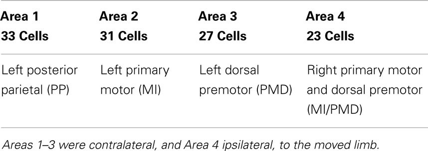
Table 1. Assignment of electrode arrays in the four cortical regions.
2.2. Statistical and Information Theoretical Analysis
If a neuron fires according to a Poisson process, then its ISI follows an exponential distribution described by
where λ > 0 is a parameter. To assess how different the distribution of ISI is from an exponential distribution, we shall also examine gamma distribution, log-normal distribution, and power-law distribution.
The gamma distribution is specified by
where parameters λ, t > 0, and Γ(t) is the gamma function:
When t is an integer (say k), the distribution is called the Erlang distribution, which governs the summation of k independent exponentially distributed random variables.
Log-normal distribution is given by
It is the distribution for the random variable Y = eX, where X has a normal (or Gaussian) distribution. To assess the goodness-of-fit of log-normal distribution to certain ISI data, one can first take logarithm of the ISI data, then check if the distribution is similar to Gaussian.
Power-law distribution can be written as
where α and b are called the shape and the location parameters, respectively. When plotted in double-logarithmic scale, such a distribution produces a straight line. To better understand the causal relation between neural inputs and movement trajectories, it is useful to analyze the correlations between them. One simple way is the cross-correlation analysis. More general correlations, including non-linear correlations, can be characterized by mutual information. To compute the dependence of cross-correlation and mutual information with time, one can partition the data into many small segments, then calculate the correlations between the corresponding segments, and finally plot the correlation against the time index associated with each segment. Let the segment of firing data of a neuron be denoted by w(t), and hand trajectory (either x, y, or z component) be denoted by u(t). The cross-correlation, denoted by C(w,u), can be calculated by the simple equation
where ⟨⟩ denotes average within the segment, and L is a small time chosen in such a way that ⟨w(t)u(t − L)⟩is maximized. When C(w,u) is normalized by the standard deviations of w(t) and u(t), one obtains the correlation coefficient. Before taking the average within each segment, one could remove the mean values of w(t) and u(t) first.
The mutual information of w(t) and u(t), written as I(w,u), is the amount of information gained about u when w is learned, and vice versa. Denote the probability distribution for w(t) by P(W = wi), i = 1, …, Nw, that for u(t) by P(U = ui), i = 1, …, Nu, and the joint distribution for w(t) and u(t) by P(W = wi, U = uj). Then
I(w,u) = 0 if and only if W and U are independent.
2.3. LRD and Multifractal Analysis
Multifractal theory provides an elegant statistical characterization of many complex dynamical variations in nature and engineering (42). There are two major types of multifractal analysis, structure function based and singular measure based (42, 43). For a relation between them, we refer to Hu et al. (44).
Within the framework of structure function based multifractal analysis, there are three techniques (42): one is the standard approach, including the Fano factor analysis; another is detrending based; the third is wavelet based. While they are equivalent when analyzing ideal fractal processes, detrending and wavelet based formulations are more reliable when analyzing real world data (43). To facilitate interpretation of our analysis below, we describe them in order here.
2.3.1. Structure function based multifractal analysis
Let X = {Xt:t = 0, 1, 2, …} be a covariance stationary stochastic process with mean μ, variance σ2, and autocorrelation function r(k), k ≥ 0. The process is said to have long-range correlation or LRD (42) if r(k) is of the form
where 0 < H < 1 is the Hurst parameter: depending on whether H is smaller than, equal to, or larger than 1/2, the process is said to have anti-persistent, short-range, or persistent long-range correlations (42, 43). Note that when 1/2 < H < 1, Σk r(k) = ∞. This justifies the term “long-range correlation” or LRD. We now consider estimation of H. A convenient framework is based on the random walk process y, defined as,
where is the mean of X. We then examine whether the following scaling laws hold or not,
where q is real and the average is taken over all possible pairs of (y(i + m), y(i)). Note that q > 0 emphasizes large absolute value, while q < 0 emphasizes small absolute value (to better understand this statement, it is helpful to think about concrete cases such as q = 10 and −10). When H(q) is a constant, the process is called a monofractal; otherwise, it is called a multifractal. The case of q = 2 is of special interest, since H(2) = H. In this case, equation (8) is often called fluctuation analysis (FA). It is equivalent to many other methods, including Fano factor analysis. In the context of ISI analysis, this can be explained as follows. Fano factor is defined as
where Ni(T) is the number of spikes in the ith window of duration T. For a Poisson process, F(T) is 1, independent of T. For a fractal process, Var[Ni(T)] ∝ T2H, while Mean[Ni(T)] ∝ T. Therefore,
In other words, Fano factor can be viewed as examining the relation between [⟨|y(i + m) − y(i)|2⟩/m] and m instead of the relation between [⟨|y(i + m) − y(i)|2⟩] and m.
2.3.2. Multifractal adaptive fluctuation analysis
When a time series is non-stationary or containing a trend, the standard structure function based approach does not work well. Our experiences with fMRI analysis (45, 46) and other applications (47) suggest that detrended fluctuation analysis (DFA) and wavelet multi-resolution analysis are more robust. Here we apply another powerful method, adaptive fluctuation analysis (AFA), which is similar to DFA but provides additional advantages over DFA (48, 49). For example, AFA can deal with arbitrary, strong non-linear trends while DFA cannot (44, 50), AFA has better resolution of fractal scaling behavior for short time series (51), AFA has a direct interpretation in terms of spectral energy while DFA does not (50), and there is a simple proof of why AFA yields the correct H while such a proof is not available for DFA (see equations (6) and (7) in Ref. (50)).
AFA works as follows (50). We first construct a random walk process from the original data using equation (7). Next, for a window size w, we determine, for the random walk process u(i) (or the original process if it is already a random walk process), a global trend v(i), i = 1, 2, …, N (44, 52, 53). Here N is the length of the random walk process. The residual, u(i) − v(i), characterizes fluctuations around the global trend, and its variance yields the Hurst parameter H,
AFA can be easily extended to MF-AFA, by extending equation (11) to a multifractal formulation,
where q is a real number: depending on whether q is positive or negative, large or small values of deviations are emphasized, respectively. In many applications, the case of q = 2 may be most concerned, since H(2) = H. For notational convenience, F(2)(w) may be simply denoted as F(w).
Equation (11) can also be extended to high-dimensional case, such as an image or a high-dimensional trajectory. In the case of 2-D, this can be achieved by first applying the algorithm to the x-component of the data, then applying it to the y-component. At least for the polynomial order 1, whether x-component first or y-component first will not make any difference, so far as functions such as d/dx d/dy f(x,y) = d/dy d/dx f(x,y).
2.3.3. Wavelet based multifractal analysis
The essence of wavelet based multifractal analysis is similar to that of adaptive multifractal analysis. Technically, it is based on the coefficients of a discrete wavelet decomposition. It involves a scaling function ϕ0 and a mother wavelet ψ0. The scaling function satisfies
The wavelet ψ0 must have zero average and decay quickly at both ends (54). The scaled and shifted versions of ϕ0 and ψ0 are given by
where j and k are the scaling (dilation) and the shifting (translation) index, respectively. Different value of j corresponds to analyzing a different resolution level of the signal. One popular technique used to perform the discrete wavelet transform (DWT) is the multiresolution analysis (MRA). The procedure of performing MRA consists of the following steps (54):
(1) At the j-th resolution, compare ϕj, k(n) and ψj, k(n) to the section at the start of the input signal x(n), this amounts to taking k = 0. Calculate the approximation coefficient ax(j,k) and the detailed coefficient dx(j,k) using the following equations
(2) Shift ϕj, k(n) and ψj, k(n) to the right, this corresponds to taking k = 1, 2, …. For each k value, repeat step (1) until the whole signal is covered.
(3) The signal approximation SAj and the signal detail SDj at the j-th resolution level are computed as
(4) Repeat steps (1) through (3) for the (j + 1)-th resolution level but use the signal approximation SAj obtained in step (2) as the input signal.
For examples detailing these steps, we refer to Hu et al. (47) and Gao et al. (42).
Let the maximum scale resolution level chosen for analysis be J. The signal can be reconstructed using the following equation (54):
The first term represents the approximation at level J, and the second term represents the details at resolution level J and lower. MRA builds a pyramidal structure that requires an iterative application of the scaling and the wavelet functions, respectively. Let
where nj is the number of coefficients at level j. For fractal signals such as the spike counting process, one has
where c0 is some constant.
Formulation based on equation (14) can be extended to wavelet based multifractal analysis, by considering
and examining whether the following scaling relations hold or not:
If yes, then we have
where each cq is some constant.
3. Results
3.1. Varying Degree of Correlation between Neuronal Firings and Hand Trajectory
To understand how neuronal firings control hand trajectory, it is instructive to visually examine the correlation between neural firings and hand trajectory. For this purpose, three consecutive hand movements are shown in Figure 1A, while neuronal firings of five neurons associated with those three hand movements are shown in Figures 1B–F. A number of interesting features can be observed from Figures 1B–F: (i) the firing rate varies considerably among the neurons. For example, neuron 1, plotted in Figure 1B, fired a lot more than most other neurons. (ii) The firing of neuron 1 of Figure 1B does not have much correlation with the hand trajectory. In fact, more than half of the neurons behaved like this. (iii) While neurons 2–4, plotted in Figures 1C–E, appear to have strong correlations with the hand movement trajectory, the degree of correlation varies with time considerably. For example, neuron 2, 3, and 4 did not fire much during the monkey’s “first,” “second,” and “third” period of hand movement, respectively. It should be mentioned that albeit neuron 5, shown in Figure 1F, fired a lot during all these three periods, it also had “quiet” periods even though the monkey was actively grabbing food to mouth. These observations suggest (i) different neurons have different degree of importance in determining the causal relation between neural inputs and hand movements, and (ii) even for the same neuron, this degree of importance varies with time considerably.
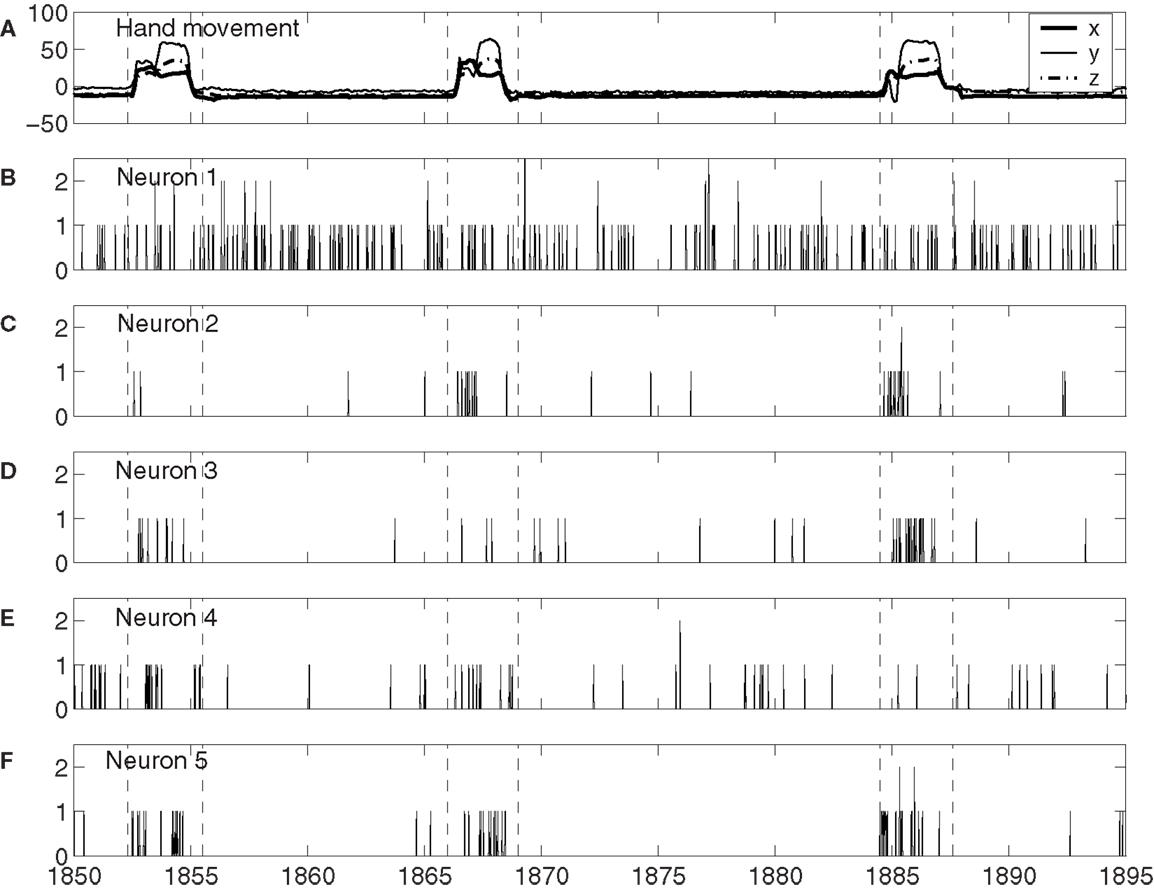
Figure 1. (A) X, Y, Z components of the monkey’s hand movements. Dashed lines indicate time intervals when the monkey stretched its hand to grab food and subsequently place the food to its mouth. (B–F) Neuronal firings of five neurons associated with the hand movements plotted in (A).
3.2. Heterogeneity of Neuronal Firings Revealed by Distributional Analysis
Conventionally, neuronal ISI data are modeled by exponential and gamma distributions. Besides these two distributions, many other distributions have been observed from the monkey’s neuronal firing data, such as log-normal and power-law distributions. Four examples are shown in Figures 2A–D, for exponential, gamma, log-normal, and power-law distributions, respectively, for four different neurons. Systematic distributional analysis of the 104 neuronal firings examined here reveals that there are 13, 21, 24, and 22 neuronal firings follow exponential, gamma, log-normal, and power-law distributions, respectively, while 24 firings could not be classified, due to lack of data. See Table 2. These distributional analyses clearly indicate that the ISI data of different neurons may follow very different distributions, and therefore, the neurons, in terms of their firing patterns, can be considered very heterogeneous. It is well-known that associated with a distribution, there is a specific stochastic process (55, 56). Existence of multiple distributions therefore implies existence of different stochastic processes underlying neuronal firings in the cortex.
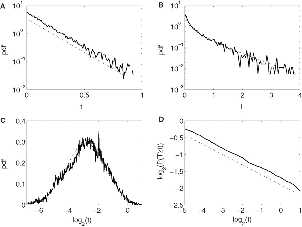
Figure 2. Four types of neuron ISI distributions. (A) Exponential, (B) gamma, (C) log-normal, and (D) power-law. Plotted in (A–C) and (D) are probability density functions (pdfs) and complementary cumulative distribution function (CCDF), respectively.
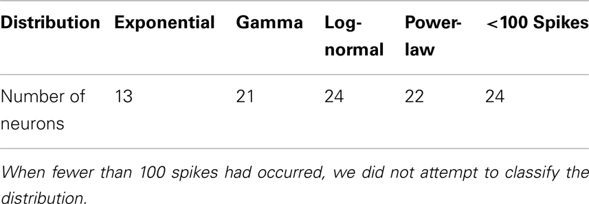
Table 2. Number of neuronal firings following exponential, gamma, log-normal, and power-law distributions.
3.3. Non-Stationary Neuronal Firings Revealed by Correlation Analysis
To quantify the time-varying correlations between the neuronal firings and movement trajectory, we computed cross-correlation coefficient and mutual information. The results are shown in Figures 3A,B, respectively. Evidently, both types of correlations vary with time considerably. Since hand trajectory is stationary, this indicates that neuronal firing patterns are highly non-stationary. The non-stationarity is one of the fundamental reasons that the accuracy of currently used adaptive models cannot be further improved.
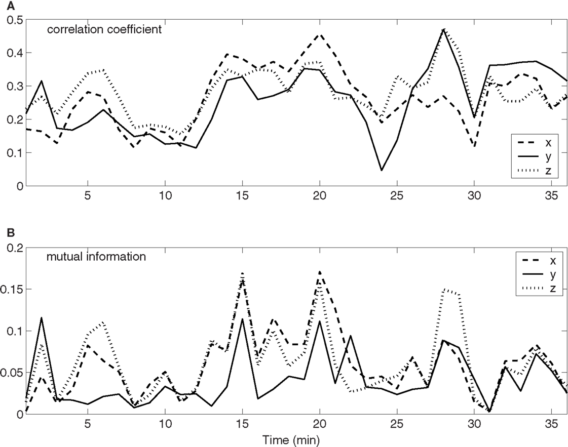
Figure 3. Time-varying correlations between spike counting data and hand movement data. (A) Correlation coefficient; (B) mutual information.
3.4. LRD in Neuronal Firings Revealed by Fano Factor Analysis
To gain insights into the distinguished features that define the set of neurons that have strong correlations with hand trajectory (i.e., neurons that are similar to those shown in Figures 1C–F), we now carry out Fano factor analysis on the counting process of spikes. For this purpose, we have classified neurons into two groups, one group is not correlated with hand movement, just as the one shown in Figure 1B, while the other group is well correlated with hand movement, as those shown in Figures 1C–F. We then have obtained the counting processes by choosing the size of the small time window to be Δt = 0.1 s. Figure 4 shows the results for six neurons, where F(T) denotes Fano factor. Note that neurons (a–c) are not well correlated with hand movement, while neurons (d–f) are. Recall that for a Poisson process, F(T) = 1, while for a fractal process, F(T) ∝ T2H − 1. Since in no cases F(T) = 1, we have to conclude that Poisson processes are not relevant here. While Figure 4 suggests fractal neuronal firings, we have to note that the power-law scaling of F(T) ∝ T2H − 1, where 2H − 1 is the slope of the plots in the Figure, are not well defined for most of the neurons. Nevertheless, H is generally greater than 1/2, especially when time scale is large. Recall that H > 1/2 indicates LRD. In the context of neuronal firings, this means that very active firing will be more likely followed by another active firing, while quiet firing will be more likely followed by another quiet firing. In other words, a small ISI will be more likely followed by another small ISI, while a large ISI will be more likely followed by another large ISI [for a similar interpretation in the context of switching times in multistable visual perception, we refer to (57, 58)]. Therefore, the firings of these neurons have LRD. However, Fano factor analysis does not clearly indicate the correlations between neuronal firings and the hand movement.
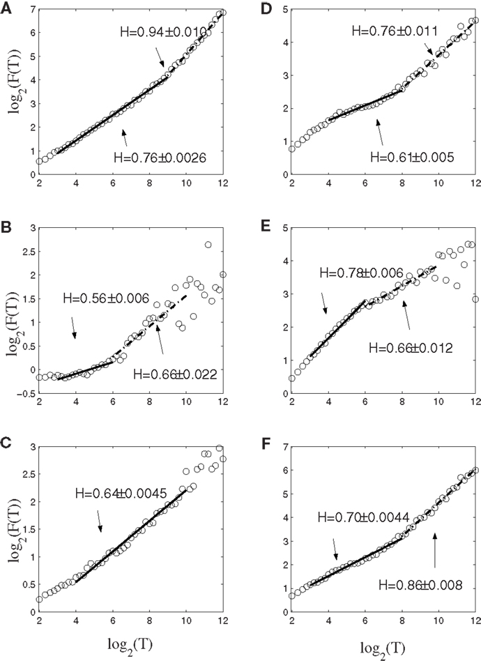
Figure 4. Fano factor analysis of the spike count data of 6 neurons, where F(T) denotes the Fano factor. The slopes in the figure amount to 2H − 1. Note that visually, neurons (A–C) are not well correlated with hand movements, while neurons (D–F) are highly correlated with hand movements.
3.5. LRD in Neuronal Firings Revealed by AFA
Next, we apply AFA to the spike counting processes of the same six neurons. The results are shown in Figure 5. Note that the slopes in the Figure correspond to H. It is observed that the lines are quite straight, therefore, the power-law relation of equation (11) is well defined. More interestingly, it is observed that three neurons, shown in Figures 5A–C, are characterized by a single fractal scaling, with the Hurst parameter ranging from about 0.5 to about 0.73, indicating no correlations or weak correlations. On the other hand, the three other neurons shown in Figures 5D–F have very large Hurst parameters, indicating very strong temporal LRD. Note that the AFA curves for those three neurons present a turning point (called fractal scaling break) at around m = 26 ∼ 27, which corresponds to about 6.4 ∼ 12.8 s. Interestingly, the time scale of 6.4 ∼ 12.8 s is comparable to the average time of 8 s between two successive reaching tasks. These two features, a large Hurst parameter, and fractal scaling break at the time scale comparable to the average time between two successive reaching tasks, suggest that neurons well correlated with hand trajectory experienced a “re-setting” effect at the start of each reaching task, in the sense that within the movement correlated neurons the spike trains’ LRD persisted about the length of time the monkey used to switch between task executions. A new task execution re-sets their activity, making them only weakly correlated with their prior activities on longer time scales. This necessitates that a difference in the detail of long-range dependence must come into being with the new task execution, breaking the LRD associated with the prior task.
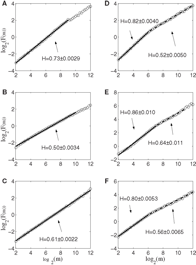
Figure 5. AFA of the same six neurons. Note that the slopes in the figure amounts to 2H. Also note that neurons (A–C) only have one scaling range, while neurons (D–F) have two scaling ranges.
3.6. LRD in Neuronal Firings Revealed by Wavelet Analysis
Figure 6 shows the result of wavelet analysis of the spike counting data of the same six neurons. We observe that the results are consistent with those based on AFA. Therefore, we can conclude that firings of the neurons well correlated with hand movements are characterized by large H with a scaling range up to the average time between two successive reaching tasks.
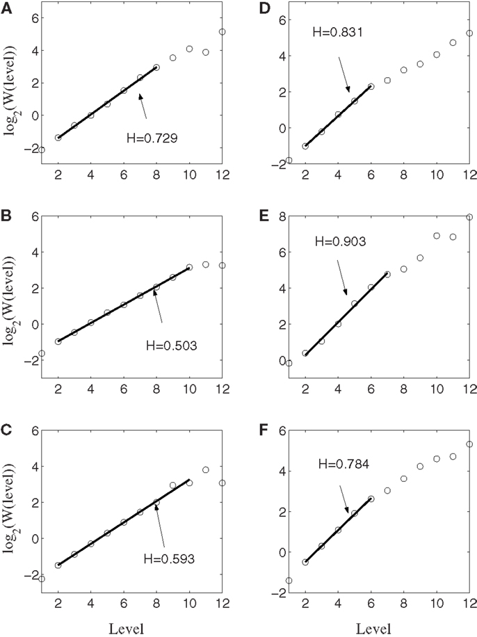
Figure 6. Wavelet analysis of the same six neurons. Here, the slope equals H. Notice the consistency with AFA analysis.
3.7. Multifractal AFA and Wavelet Analysis of Superimposed Neuronal Firings
To examine whether the neurons in the four brain areas (Table 1) may have different fractal properties, we combined the neuronal firings in each brain area and obtained a “superimposed” spike train, and then performed multifractal analysis based on MF-AFA and multifractal wavelet analysis. The results are shown in Figures 7 and 8, respectively. Recalling that multifractal is characterized by a non-constant H(q), while a monofractal is characterized by a fairly constant H(q), we conclude that areas 1 and 4 show multifractal behavior, while areas 2 and 3 show weak multifractal or monofractal behavior. This suggests that different brain areas may have different roles in coordinating movements.
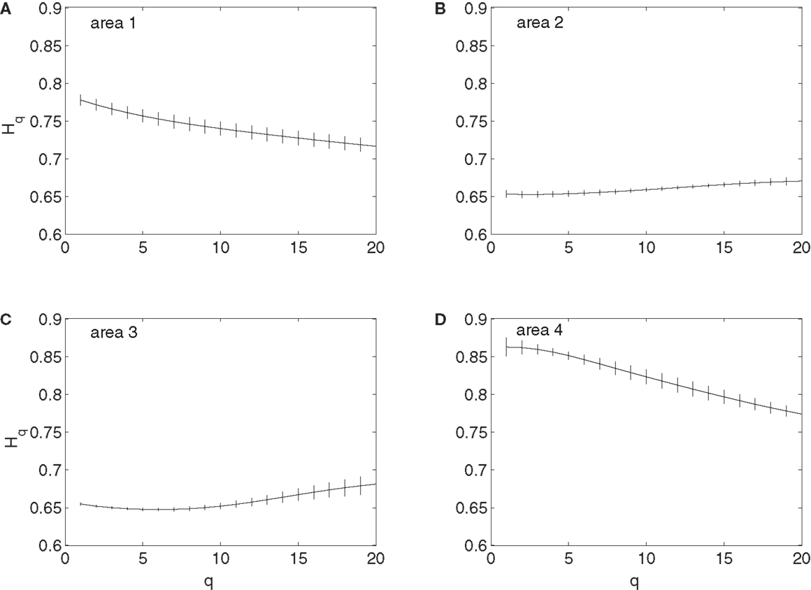
Figure 7. MF-AFA of the “superimposed” spike train in the four brain areas, where (A) for area 1, left posterior parietal (PP); (B) area 2, left primary motor (MI); (C) area 3, left dorsal premotor (PMD); and (D) area 4, right primary motor and dorsal premotor (MI/PMD).
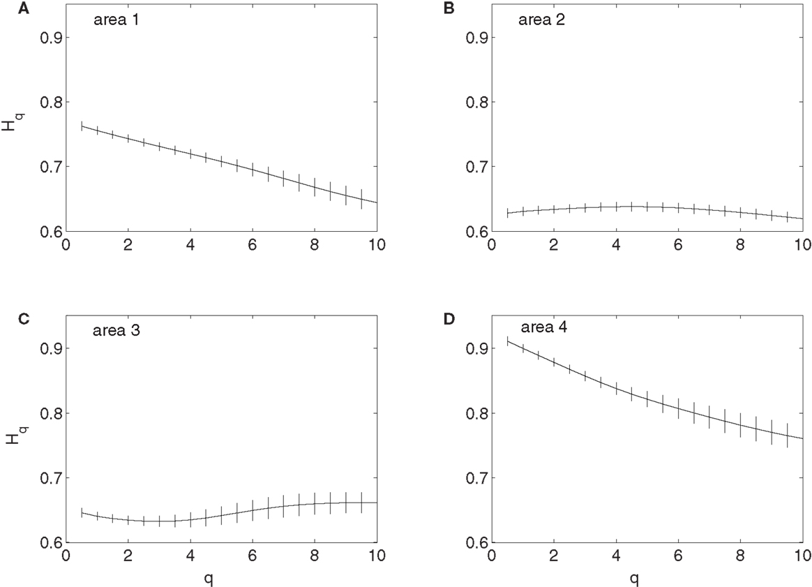
Figure 8. MF wavelet analysis of the “superimposed” spike train in the four brain areas, where (A) for area 1, left posterior parietal (PP); (B) area 2, left primary motor (MI); (C) area 3, left dorsal premotor (PMD); and (D) area 4, right primary motor and dorsal premotor (MI/PMD).
3.8. Important vs. Irrelevant Neurons
Although 104 neurons have been analyzed here, there are only slightly more than 10 neurons that exhibit the interesting fractal scalings discussed above, and thus can be classified as important neurons. Amazingly, when those neurons are used to train a Wiener filter, the simulated trajectory already achieves about 65% correlation with the actual hand trajectory. However, when similar number of other neurons are used to predict a trajectory, the correlation between the predicted trajectory and the actual trajectory becomes very poor. Therefore, those neurons are indeed the most important in reaching tasks.
4. Discussions
To better understand the causal relation between neural inputs and movements, in this study, we have employed three different types of fractal and multifractal techniques, including Fano factor analysis, multifractal adaptive fluctuation analysis (MF-AFA), and wavelet multifractal analysis, to study whether neuronal firings related to movements may have LRD. We find that Fano factor analysis always indicates LRD in neuronal firings, irrespective of whether those firings are correlated with movement trajectory or not. Therefore, Fano factor analysis, while indicating that neuronal firings related to movements are generally non-Poisson, does not reveal any actual correlations between neural inputs and movements. This may be due to the overwhelming non-stationarity nature of neuronal firings. More interestingly, we have found that MF-AFA and wavelet multifractal analysis can clearly indicate that when neuronal firings are not well correlated with movement trajectory, they only have weak or very short-range temporal correlations. When neuronal firings are well correlated with movements, they are characterized by very strong temporal correlations, up to a time scale comparable to the average time between two successive reaching tasks. Beyond that time scale, LRD no longer exists. This suggests that neurons well correlated with hand trajectory experienced a re-setting effect at the start of each reaching task, in the sense that within the movement correlated neurons the spike trains’ LRD persisted about the length of time the monkey used to switch between task executions. A new task execution re-sets their activity, making them only weakly correlated with their prior activities on longer time scales. This necessitates that a difference in the detail of long-range dependence must come into being with the new task execution, breaking the LRD associated with the prior task.
The existence of a group of neurons whose firings are well correlated with hand movement suggests that neural information processing is carried out by a dynamic coalition of neurons, as hypothesized by Edelman and Tononi (59), Crick and Koch (60), Gao et al. (57), and Furstenau (61). By a coalition of neurons, it is meant that the coalition involves many types of excitatory and inhibitory interconnected neurons, which change the activities of their fellow members. By dynamic, it is meant that neurons within the coalition may leave the coalition and not participate in neural information processing, such as controlling hand movements. After they leave the coalition, they may re-join the coalition later; or new neurons can join the coalition. To better understand these statements, we note that in the time interval of three hand movements shown in Figure 1, if we define the dynamic coalition of neurons by their correlation with the hand trajectory, then neuron 1 does not belong to the coalition, neuron 5 belongs to the coalition, and neurons 2 to 4 are transient members – they do not belong to the coalition at the 1st, 2nd, and 3rd hand movement, respectively. This dynamic aspect is also responsible for the re-setting aspect of the important neurons discussed earlier. While the process of leaving and joining the coalition makes the structure of the network of the coalition highly time-varying, the collective behavior of the coalition must be fairly stable, since it controls movements. It is interesting to note that the notion of soft assemble proposed by Turvey (62) and the hypothesis of self-organization perception and action proposed by Van Orden et al. (63) are consistent with the framework discussed here.
The above discussion highly suggests that understanding the collective behavior of the coalition of neurons will be critical for fully realizing the promises of BMIs. One testable idea is to select neurons having relatively large Hurst parameters for adaptation algorithms thereby reducing the number of free parameters. Our own experience, as described in the last section, suggests that this is a valid idea. This is also consistent with the work of Sanchez et al. (26). The best predictions by adaptive algorithms may be obtained by not only using the notion of LRD, but also the notion of “dynamic” or “non-stationary.” By the latter, we mean that when a neuron has left the coalition of neurons performing a desired task, it then should be removed in the adaptive algorithm for prediction.
Conflict of Interest Statement
The authors declare that the research was conducted in the absence of any commercial or financial relationships that could be construed as a potential conflict of interest.
Acknowledgments
The authors thank Dr. Nicolelis for providing the neuronal firing data.
References
1. Andersen RA, Musallam S, Pesaran B. Selecting the signals for a brain-machine interface. Curr Opin Neurobiol (2004) 14:720–6. doi:10.1016/j.conb.2004.10.005
2. Donoghue JP. Bridging the brain to the world: a perspective on neural interface systems. Neuron (2008) 60:511–21. doi:10.1016/j.neuron.2008.10.037
3. Waldert S, Preissl H, Demandt E, Braun C, Birbaumer N, Aertsen A, et al. Hand movement direction decoded from MEG and EEG. J Neurosci (2008) 28:1000–8. doi:10.1523/JNEUROSCI.5171-07.2008
4. Schalk G, Kubanek J, Miller KJ, Anderson NR, Leuthardt EC, Ojemann JG, et al. Decoding two-dimensional movement trajectories using electrocorticographic signals in humans. J Neural Eng (2007) 4:264–75. doi:10.1088/1741-2560/4/3/012
5. Stark E, Abeles M. Predicting movement from multiunit activity. J Neurosci (2007) 27:8387–94. doi:10.1523/JNEUROSCI.1321-07.2007
6. Schwartz AB, Cui XT, Weber DJ, Moran DW. Brain-controlled interfaces: movement restoration with neural prosthetics. Neuron (2006) 52:205–20. doi:10.1016/j.neuron.2006.09.019
7. Hochberg LR, Serruya MD, Friehs GM, Mukand JA, Saleh M, Caplan AH, et al. Neuronal ensemble control of prosthetic devices by a human with tetraplegia. Nature (2006) 442:164–71. doi:10.1038/nature04970
8. Rickert J, de Oliveira SC, Vaadia E, Aertsen A, Rotter S, Mehring C. Encoding of movement direction in different frequency ranges of motor cortical local field potentials. J Neurosci (2005) 25:8815–24. doi:10.1523/JNEUROSCI.0816-05.2005
9. Georgopoulos AP, Schwartz AB, Kettner RE. Neuronal population coding of movement direction. Science (1986) 233:1416–9. doi:10.1126/science.3749885
10. Chapin JK, Moxon KA, Markowitz RS, Nicolelis MAL. Real-time control of a robot arm using simultaneously recorded neurons in the motor cortex. Nat Neurosci (1999) 2:664–70. doi:10.1038/10223
11. Wessberg J, Stambaugh CR, Kralik JD, Beck PD, Laubach M, Chapin JK, et al. Real-time prediction of hand trajectory by ensembles of cortical neurons in primates. Nature (2000) 408:361–5. doi:10.1038/35042582
12. Schwartz AB, Taylor DM, Tillery SIH. Extraction algorithms for cortical control of arm prosthetics. Curr Opin Neurobiol (2001) 11:701–7. doi:10.1016/S0959-4388(01)00272-0
13. Serruya MD, Hatsopoulos NG, Paninski L, Fellows MR, Donoghue JP. Instant neural control of a movement signal. Nature (2002) 416:141–2. doi:10.1038/416141a
14. Taylor DM, Tillery SIH, Schwartz AB. Direct cortical control of 3D neuroprosthetic devices. Science (2002) 296:1829–32. doi:10.1126/science.1070291
15. Carmena JM, Lebedev MA, Crist RE, O’Doherty JE, Santucci DM, Dimitrov DF, et al. Learning to control a brain-machine interface for reaching and grasping by primates. PLoS Biol (2003) 1(2):e42. doi:10.1371/journal.pbio.0000042
16. Wu W, Black MJ, Mumford D, Gao Y, Bienenstock E, Donoghue JP. Modeling and decoding motor cortical activity using a switching Kalman filter. IEEE Trans Biomed Eng (2004) 6:933–42. doi:10.1109/TBME.2004.826666
17. Wu W, Gao Y, Bienenstock E, Donoghue JP, Black MJ. Bayesian population decoding of motor cortical activity using a Kalman filter. Neural Comput (2006) 18:80–118. doi:10.1162/089976606774841585
18. Li Z, O’Doherty JE, Lebedev MA, Nicolelis MA. Adaptive decoding for brain-machine interfaces through Bayesian parameter updates. Neural Comput (2011) 23:3162–204. doi:10.1162/NECO_a_00207
19. Hauschild M, Mulliken GH, Fineman I, Loeb GE, Andersen RA. Cognitive signals for brain-machine interfaces in posterior parietal cortex include continuous 3D trajectory commands. Proc Natl Acad Sci U S A (2012) 16:17075–80. doi:10.1073/pnas.1215092109
20. Shanechi MM, Williams ZM, Wornell GW, Hu RC, Powers M, Brown EN. A real-time brain-machine interface combining motor target and trajectory intent using an optimal feedback control design. PLoS One (2013) 8:e59049. doi:10.1371/journal.pone.0059049
21. Wiener N. Extrapolation, Interpolation, and Smoothing of Stationary Time Series with Engineering Applications. Cambridge, MA: MIT press (1949).
25. Kim SP, Sanchez JC, Erdogmus D, Rao YN, Wessberg J, Principe JC, et al. Divide-and-conquer approach for brain machine interfaces: nonlinear mixture of competitive linear models. Neural Netw (2003) 16:865–71. doi:10.1016/S0893-6080(03)00108-4
26. Sanchez JC, Carmena JM, Lebedev MA, Nicolelis MAL, Harris JG, Principe JC. Ascertaining the importance of neurons to develop better brain-machine interfaces. IEEE Trans Biomed Eng (2004) 51:943–53. doi:10.1109/TBME.2004.827061
27. Sanchez JC, Erdogmus D, Nicolelis MAL, Wessberg J, Principe JC. Interpreting spatial and temporal neural activity through a recurrent neural network brain-machine interface. IEEE Trans Neural Syst Rehabil Eng (2005) 13:213–9. doi:10.1109/TNSRE.2005.847382
28. Teich MC. Fractal character of the auditory neural spike train. IEEE Trans Biomed Eng (1989) 36:150–60. doi:10.1109/10.16460
29. Teich MC, Lowen SB. Fractal patterns in auditory nerve-spike trains. IEEE Eng Med Biol Mag (1994) 13:197–202. doi:10.1109/51.281678
30. Turcott RG, Barker PDR, Teich MC. Long-duration correlation in the sequence of action potentials in an insect visual interneuron. J Stat Comput Simul (1995) 52:253–71. doi:10.1080/00949659508811677
31. Teich MC, Turcott RG, Siegel RM. Temporal correlation in cat striate-cortex neural spike trains. IEEE Eng Med Biol Mag (1996) 15:79–87. doi:10.1109/51.537063
32. Teich MC, Heneghan C, Lowen SB, Ozaki Y, Kaplan E. Fractal character of the neural spike train in the visual system of the cat. J Opt Soc Am A (1997) 14:529–46. doi:10.1364/JOSAA.14.000529
33. Baddeley R, Abbott LF, Booth MC, Sengpiel F, Freeman T, Wakeman EA, et al. Responses of neurons in primary and inferior temporal visual cortices to natural scenes. Proc Biol Sci (1997) 264:1775–83. doi:10.1098/rspb.1997.0246
34. Lewis CD, Gebber GL, Larsen PD, Barman SM. Long-term correlations in the spike trains of medullary sympathetic neurons. J Neurophysiol (2001) 85:1614–22.
35. Das M, Gebber GL, Barman SM, Lewis CD. Fractal properties of sympathetic nerve discharge. J Neurophysiol (2003) 89:833–40. doi:10.1152/jn.00757.2002
36. Ratnam R, Nelson ME. Nonrenewal statistics of electrosensory afferent spike trains: implications for the detection of weak sensory signals. J Neurosci (2000) 120:6672–83.
37. Orer HS, Das MS, Barman SM, Gebber GL. Fractal activity generated independently by medullary sympathetic premotor and preganglionic sympathetic neurons. J Neurophysiol (2003) 90:47–54. doi:10.1152/jn.00066.2003
38. Nelson ME. Multiscale spike train variability in primary electrosensory afferents. J Physiol Paris (2002) 96:507–16. doi:10.1016/S0928-4257(03)00006-8
39. Bhattacharya J, Edwards J, Mamelak AN, Schuman EM. Long-range temporal correlations in the spontaneous spiking of neurons in the hippocampal-amygdala complex of humans. Neuroscience (2005) 131:547–55. doi:10.1016/j.neuroscience.2004.11.013
40. Zheng Y, Gao JB, Sanchez JC, Principe JC, Okun MS. Multiplicative multifractal modeling and discrimination of human neuronal activity. Phys Lett A (2005) 344:253–64. doi:10.1016/j.physleta.2005.06.092
41. Nicolelis MAL, Ghazanfar AA, Faggin BM, Votaw S, Oliveira LMO. Reconstructing the engram: simultaneous, multisite, many single neuron recordings. Neuron (1997) 18:529–37. doi:10.1016/S0896-6273(00)80295-0
42. Gao J, Cao Y, Tung W, Hu J. Multiscale Analysis of Complex Time Series – Integration of Chaos and Random Fractal Theory, and Beyond. Hoboken, NJ: Wiley Interscience (2007).
43. Gao JB, Hu J, Tung WW, Cao YH, Sarshar N, Roychowdhury VP. Assessment of long range correlation in time series: how to avoid pitfalls. Phys Rev E Stat Nonlin Soft Matter Phys (2006) 73:016117. doi:10.1103/PhysRevE.73.016117
44. Hu J, Gao JB, Wang XS. Multifractal analysis of sunspot time series: the effects of the 11-year cycle and Fourier truncation. J Stat Mech (2009). doi:10.1088/1742-5468/2009/02/P02066
45. Hu J, Lee JM, Gao JB, White KD, Crosson B. Assessing a signal model and identifying brain activity from fMRI data by a detrending-based fractal analysis. Brain Struct Funct (2008) 212:417–26. doi:10.1007/s00429-007-0166-9
46. Lee JM, Hu J, Gao JB, Crosson B, Peck KK, Wierenga CE, et al. Discriminating brain activity from task-related artifacts in functional MRI: fractal scaling analysis simulation and application. Neuroimage (2008) 40:197–212. doi:10.1016/j.neuroimage.2007.11.016
47. Hu J, Gao JB, Posner FL, Zheng Y, Tung WW. Target detection within sea clutter: a comparative study by fractal scaling analyses. Fractals (2006) 14:187–204. doi:10.1142/S0218348X06003210
48. Riley MA, Kuznetsov N, Bonnette S, Wallot S, Gao JB. A tutorial introduction to adaptive fractal analysis. Front Fractal Physiol (2012) 28:371. doi:10.3389/fphys.2012.00371
49. Kuznetsov N, Bonnette S, Gao JB, Riley MA. Adaptive fractal analysis reveals limits to fractal scaling in center of pressure trajectories. Ann Biomed Eng (2012) 41:1646–60. doi:10.1007/s10439-012-0646-9
50. Gao JB, Hu J, Tung WW. Facilitating joint chaos and fractal analysis of biosignals through nonlinear adaptive filtering. PLoS One (2011) 6:e24331. doi:10.1371/journal.pone.0024331
51. Gao JB, Hu J, Mao X, Perc M. Culturomics meets random fractal theory: insights into long-range correlations of social and natural phenomena over the past two centuries. J R Soc Interface (2012) 9:1956–64. doi:10.1098/rsif.2011.0846
52. Gao JB, Sultan H, Hu J, Tung WW. Denoising nonlinear time series by adaptive filtering and wavelet shrinkage: a comparison. IEEE Signal Process Lett (2010) 17:237–40. doi:10.1109/LSP.2009.2037773
53. Tung WW, Gao JB, Hu J, Yang L. Recovering chaotic signals in heavy noise environments. Phys Rev E Stat Nonlin Soft Matter Phys (2011) 83:046210. doi:10.1103/PhysRevE.83.046210
55. Grimmett G, Stirzaker D. Probability and Random Processes. 3rd ed. Oxford: Oxford University Press (2001).
57. Gao JB, Billock VA, Merk I, Tung WW, White KD, Harris JG, et al. Inertia and memory in ambiguous visual perception. Cogn Process (2006) 7:105–12. doi:10.1007/s10339-006-0030-5
58. Zhou YH, Gao JB, White KD, Merk I, Yao K. Perceptual dominance time distributions in multistable visual perception. Biol Cybern (2004) 90:256–63. doi:10.1007/s00422-004-0472-8
60. Crick F, Koch C. A framework for consciousness. Nat Neurosci (2003) 6:119–26. doi:10.1038/nn0203-119
61. Furstenau N. A nonlinear dynamics model for simulating correlations of cognitive bistability. Biol Cybern (2010) 103:175–98. doi:10.1007/s00422-010-0388-4
62. Turvey MT. Action and perception at the level of synergies. Hum Mov Sci (2007) 26:657–97. doi:10.1016/j.humov.2007.04.002
Keywords: brain-machine interface, Fano factor, adaptive fluctuation analysis, wavelet, neuronal firings
Citation: Hu J, Zheng Y and Gao J (2013) Long-range temporal correlations, multifractality, and the causal relation between neural inputs and movements. Front. Neurol. 4:158. doi: 10.3389/fneur.2013.00158
Received: 28 July 2013; Paper pending published: 14 August 2013;
Accepted: 24 September 2013; Published online: 09 October 2013.
Edited by:
Olivier Darbin, University South Alabama, USAReviewed by:
John G. Holden, University of Cincinnati, USAKeith D. White, University of Florida, USA
Copyright: © 2013 Hu, Zheng and Gao. This is an open-access article distributed under the terms of the Creative Commons Attribution License (CC BY). The use, distribution or reproduction in other forums is permitted, provided the original author(s) or licensor are credited and that the original publication in this journal is cited, in accordance with accepted academic practice. No use, distribution or reproduction is permitted which does not comply with these terms.
*Correspondence: Jianbo Gao, Institute of Complexity Science and Big Data Technology, Guangxi University, 100 Daxue Road, Nanning 530005, China e-mail:amJnYW8ucG1iQGdtYWlsLmNvbQ==