- 1 Signal Processing Laboratory 5, Ecole Polytechnique Fédérale de Lausanne, Lausanne, Switzerland
- 2 Department of Radiology, University Hospital Center and University of Lausanne, Lausanne, Switzerland
Advanced neuroinformatics tools are required for methods of connectome mapping, analysis, and visualization. The inherent multi-modality of connectome datasets poses new challenges for data organization, integration, and sharing. We have designed and implemented the Connectome Viewer Toolkit – a set of free and extensible open source neuroimaging tools written in Python. The key components of the toolkit are as follows: (1) The Connectome File Format is an XML-based container format to standardize multi-modal data integration and structured metadata annotation. (2) The Connectome File Format Library enables management and sharing of connectome files. (3) The Connectome Viewer is an integrated research and development environment for visualization and analysis of multi-modal connectome data. The Connectome Viewer’s plugin architecture supports extensions with network analysis packages and an interactive scripting shell, to enable easy development and community contributions. Integration with tools from the scientific Python community allows the leveraging of numerous existing libraries for powerful connectome data mining, exploration, and comparison. We demonstrate the applicability of the Connectome Viewer Toolkit using Diffusion MRI datasets processed by the Connectome Mapper. The Connectome Viewer Toolkit is available from http://www.cmtk.org/
1 Introduction
What nervous systems do – essentially – is to connect. Investigations into the connectivity properties of nervous systems have a long history (Douglas and Martin, 2007; Fishman, 2007). Despite many efforts, contemporary knowledge about the specificity of structural and functional connectivity is still poor. The new field of connectomics is emerging to tackle the challenge of mapping complete neural circuitry, or connectomes.
Connectomes represent the fundamental pathways on which complex spatiotemporal activity patterns evolve. In turn, these activity patterns modify underlying structural pathways. For an understanding of how activity patterns arise (physiology) and what they are able to produce and mean (behavior), it is indispensable to have connectome data (neuroanatomy) on all spatial descriptive levels.
On the cellular level of description, light, and electron microscopy are the main imaging tools for mapping neuronal circuitry. Partial and complete connectomes have been mapped in a variety of organisms and structures such as the nematode Caenorhabditis elegans (Ward et al., 1975; White et al., 1976), the crustacean Daphnia’s optic lobe (Macagno et al., 1979), cat visual cortex (Binzegger et al., 2004), macaque (Felleman and Van Essen, 1991; Markov et al., 2010), the rabbit retina (Anderson et al., 2011), the mouse interscutularis muscle (Lu et al., 2009), hippocampus (Ascoli, 2010), or Drosophila melanogaster (Cardona et al., 2010; Chklovskii et al., 2010; Hampel et al., 2011).
On the macroscale level of description, diffusion-weighted magnetic resonance imaging (MRI) is the main imaging technology employed for mapping the structural connectivity of the human connectome (Hagmann, 2005; Sporns et al., 2005; Sporns, 2011). Magnetic resonance connectomics (Hagmann et al., 2010) is increasingly recognized as a tool for basic and clinical neuroscience. Several methodological advances in image acquisition, reconstruction, and tractography (Wedeen et al., 2008; Johansen-Berg and Behrens, 2009) suggest that automated processing pipelines will make it possible to generate comprehensive in vivo whole brain statistical connectomes.
Despite the big differences in spatial scale and data size, both levels of connectome mapping consist of similar stages. Connectome mapping workflows involve image acquisition, registration and segmentation, data organization and sharing, high-throughput pipelining, analysis, and visualization. Advanced neuroinformatics tools will be required to meet challenges that each stage presents. In this article, we will focus on the development of neuroinformatics tools in the emerging field of macroscale connectomics.
The efficiency of sharing data and source code would benefit if a transdisciplinary lingua franca for programming was available. Especially in the neurosciences, where researchers with varying degrees of scientific knowledge and programming skills meet, a common programming language helps to bridge gaps between theoretical and experimental worlds of investigation. Moreover, the programming language must be high-level, cross-platform, easy-to-learn, and have a large number of scientific libraries available. In recent years, Python1 has become a viable alternative to Matlab, Java, or C++. More and more, Python is becoming the language of choice in scientific computing communities (Oliphant, 2007; Langtangen, 2009). Python is a free, open source, cross-platform programming language with a rapidly growing number of high-quality scientific libraries and interfaces to legacy code. A special-topic issue on “Python in neuroscience” in Frontiers in Neuroinformatics, and a number of publications (Kinser, 2008; Spacek et al., 2008; Davison et al., 2009) give an indication of the significance of the Python programming language.
Due to improved data acquisition methods, it is now possible to acquire large multi-modal datasets in projects involving thousands of subjects. For instance, the Human Connectome Project2 is currently underway and collects Diffusion MRI, fMRI, EEG, MEG, behavioral, and genetic data in a cohort of 1200 healthy subjects. In such large-scale projects, the neuroinformatics challenges of data handling, sharing, and analysis become unnecessarily difficult without common infrastructure and data format standards. Due to their longer tradition, in the fields of volume-based and surface-based analysis in neuroimaging, standardized data formats have already been established such as NIFTI3 for volume-based data and GIFTI4 for surface-based data. Importantly for MR connectomics, no common format for network-based data yet exists. To approach the task of specifying such a format for connectivity-related neuroimaging data, the Connectivity InFormatics Technology Initiative (CIFTI) was launched. Furthermore, a dedicated program of the International Neuroinformatics Coordinating Facility (INCF5) on standards for data and metadata sharing was established.
For data management and sharing of large and multi-faceted datasets, a flexible data format is necessary. The key requirements of such a flexible data format under the macroscale connectomics perspective are severalfold:
⊳ A standardized container format for raw and processed multi-modal datasets that is based on common neuroimaging data formats, extended by a standard format for network-based datasets.
⊳ A minimal set of required metadata that can be extended flexibly by user-defined metadata, and that allow easy sharing of data and metadata across collaborating groups.
⊳ The possibility of relating different data modalities to each other.
⊳ An interface to database infrastructures.
⊳ A mapping to an object model in common programming languages.
⊳ To enable the storage of behavioral data.
⊳ To enable the storage of provenance information such as processing scripts and runtime environment
⊳ The ability to link data and concepts to semantic frameworks.
⊳ To enable easier data visualization (Benger, 2009) and analysis.
To establish a novel data format, it must come with appropriate libraries for reading and writing. Only when it is possible to easily read, modify, and save data in the new format, does it benefit the researcher who wants to focus on analysis and visualization. There exist many standard formats for the different data modalities, but no one has yet tried to combine these multi-modal datatypes into a single format.
Complementary to common data formats, investigators in the field of macroscale connectomics will require interactive research and development environments for data analysis and visualization. An optimal solution would be an integrated neuroinformatics environment based on Python. It would need to provide a graphical user interface (GUI) with extensive libraries, an interactive scripting shell and built-in script editors with code-highlighting and debugging functionality. Graph analysis libraries are required to unravel the complex brain network organization of structural and functional systems (Bullmore and Sporns, 2009). Furthermore, such a macroscale connectomics research environment needs to support an interactive mode of analysis and visualization of multi-modal datasets. Scripting interfaces provide the required flexibility to allow the implementation of a variety of multi-modal data exploration and data mining strategies in an interactive way (Akil et al., 2011). The environment needs not only to provide a methodology to automatically perform elementary functionality, but also guidance for the performance of more complex analysis and visualization tasks. Moreover, a modular software architecture fosters contributions by the open source research community. Open interfaces facilitate the reuse of a diversity of tools and external libraries that the connectome researcher can draw from.
We used the Python programming language to develop the free and open source Connectome Viewer Toolkit. We specify the Connectome File Format (CFF) as a container data format for multi-modal neuroimaging datasets, specifying a connectome file. We present the Python-based Connectome File Format Library (cfflib) for data manipulation and data sharing of connectome files. The Connectome Viewer provides a framework for interactive visualization and analysis of connectomes and multi-modal datasets. We will illustrate the application of the Connectome Viewer Toolkit on Diffusion MRI datasets processed by the Connectome Mapper. The Connectome Mapper is a Python-based tool that currently implements structural connectome mapping. Figure 1 summarizes the general connectome processing workflow for structural and functional data. It highlights the use of the Connectome Viewer tools presented in this article.
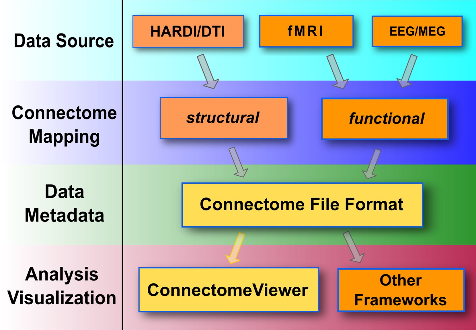
Figure 1. General processing stages of a connectome workflow. The Connectome Viewer Toolkit currently supports the workflow highlighted in yellow. Mapping streams for structural data, such as the Connectome Mapper, or functional data may converge to a connectome file and can be further managed, analyzed, and visualized with the Connectome Viewer. Connectome files may be reused in other frameworks for analysis and visualization tasks.
2 Toolkit Design
After having outlined the key neuroinformatic challenges when developing tools for macroscale connectomics, we present the design and implementation of the Python-based Connectome Viewer Toolkit for data organization, analysis, and visualization of connectome data.
General considerations We have adhered to best-practices for open source scientific software tool development from the beginning (Baxter et al., 2006). Python provides mature software engineering tools for writing, testing, debugging, and maintaining scientific software. We have followed a very modular philosophy when designing the tools and the toolkit in general.
We have adopted the powerful and widely used distributed version control system called git (Chacon, 2009). It is complemented by its biggest hosting platform GitHub6. We use GitHub as a project management platform for the support of all stages of the collaborative software development process. Our GitHub organization repositories are used for source code hosting, bug tracking, release management, code review, wiki, and visualization of the version control history and contributions.
We use the Sphinx tool7 to create the online documentation for all tools. Sphinx uses so-called restructured text as its markup language, allowing one easily to create HTML, and PDF documentation with cross-referencing. The built-in syntax highlighting of code improves the readability of the documentation. Moreover, we provide user guides, tutorials, and example datasets for all tools.
Installation For proper software packaging and distribution, the NeuroDebian project8 provides professional expertise and infrastructure. NeuroDebian provides a repository of neuroscience-related packages for easy installation on Debian-based Linux operating systems, such as Ubuntu. The Connectome Viewer Toolkit is distributed through the NeuroDebian repository, thereby facilitating the installation of dependencies and regular updates. For users on Windows or Mac OS X platforms, the Enthought Python Distribution9 provides the required Python environment for the toolkit. The Enthought Python Distribution is free for academic purposes.
2.1 The Connectome File Format
The metaphor of a container shall serve to explain how the Connectome File Format (CFF) is structured. The CFF makes a distinction between two entities: the Connectome Markup Language file and the connectome objects. The Connectome Markup Language file is a single XML-based file named meta.cml, containing metadata and a list of connectome objects. The schema for the Connectome Markup Language file is specified in conformance to the W3C standard XML schema 1.0 language (Thompson et al., 2004) and is available online. Figure 2 illustrates the basic design of the CFF graphically.
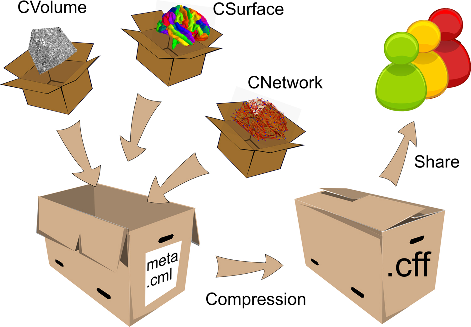
Figure 2. The Connectome File Format Container. The connectome objects with reference to their primary data and metadata are depicted as small boxes. They are stored in a connectome file, represented by the open big box. After data manipulation, the connectome file can be compressed and shared with collaborators or sent to databases.
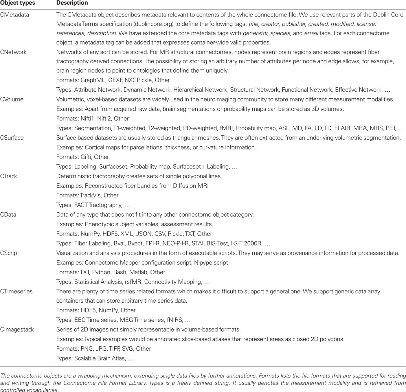
We take advantage of the power and flexiblity inherent in defining objects with XML to specify connectome objects. Connectome objects wrap data files of multiple modalities. They add a layer of metadata information to the primary data file they refer to. Each connectome object holds information about its name, fileformat, datatype, description, and additionally a flexibly extensible metadata tag. We use the term multi-modal here to distinguish data types rather than measurement modalities. The basic categories of connectome objects are: CMetadata, CNetwork, CVolume, CSurface, CTrack, CData, CScript, CTimeseries, and CImagestack. Table 1 describes the connectome object types in detail.
The connectome file is not confined to contain multi-modal datasets for a single datasets, but it can store multi-subject datasets. When storing multi-subject datasets, adding metadata annotation tags of the subject ids is suggested. Retrieving connectome objects grouped by the subject ids is then enabled by the grouping function group_by_tagkey as shown below in the listing of Section 2.2 Similarly, when individual connectome objects are tagged as belonging to a patient or control group, retrieving the corresponding datasets for group-wise comparison is possible with the same function.
Open Metadata Flexible annotation of metadata for each connectome object is enabled by the metadata tag. It is possible to annotate every connectome object in the container in the same way. We defined two ways to create annotations of metadata: (a) by simple tagging, (b) by structured annotation.
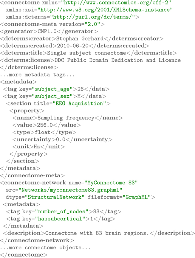
For (a), simple key-value pairs of the form <tag key=”number_of_nodes”>83</tag> are used to tag connectome objects. The employed keys can be used later on to group required objects easily in Python’s so-called dictionaries. For instance, CNetwork objects can be grouped by their number of nodes, or connectome objects of multiple subjects can be grouped based on the subject id key. Although this scheme is very handy for everyday analysis, it is often desirable to store more structured metadata. As for (b), we adopted the Open Metadata Markup Schema odML10 that was created to represent metadata for neurophysiology data in a bottom-up fashion. For metadata annotation, there are named sections that contain properties. The properties have a name and value, and additionally type, unit, and uncertainty information. This bottom-up scheme is very flexible and extensible and does not make any assumption about the terminology used. These terminologies are expected to emerge as the researchers start to annotate connectome objects using open metadata markup. Existing controlled vocabularies can already be employed with this schema. An example of the application of the metadata tag to the CMetadata object is shown in the Section 3 in Figure 6.
Multi-Modal Data Integration A connectome file can contain connectome objects for multiple modalities. These modalities are related to each other using unique numeric identifiers. Any given entity such as a brain structure or region of interest can potentially be represented in different modalities. Geometrically, an entity is instantiated as a set of cortical voxels in a volume and/or as a particular set of triangles in a surface mesh. The same entity may be represented by a node in a network.
We use integer values to establish this three-way relationship. Each entity is given a unique integer value. For each modality, this particular integer value is stored at defined places. For the CVolume object, the values are stored in individual voxels, thereby defining a segmentation. For the CSurface object, the values are stored as labelings on the vertices or on the faces, defining a surface-based parcellation. For the CNetwork object, we store the integer value as a node property. In Figure 3, we use the key dn_correspondence_id to store the integer value for a CNetwork object represented in the GraphML format11. In later analysis and visualization stages, the relevant data in the different modalities can be retrieved and combined as needed. Figure 4 depicts this schema graphically.
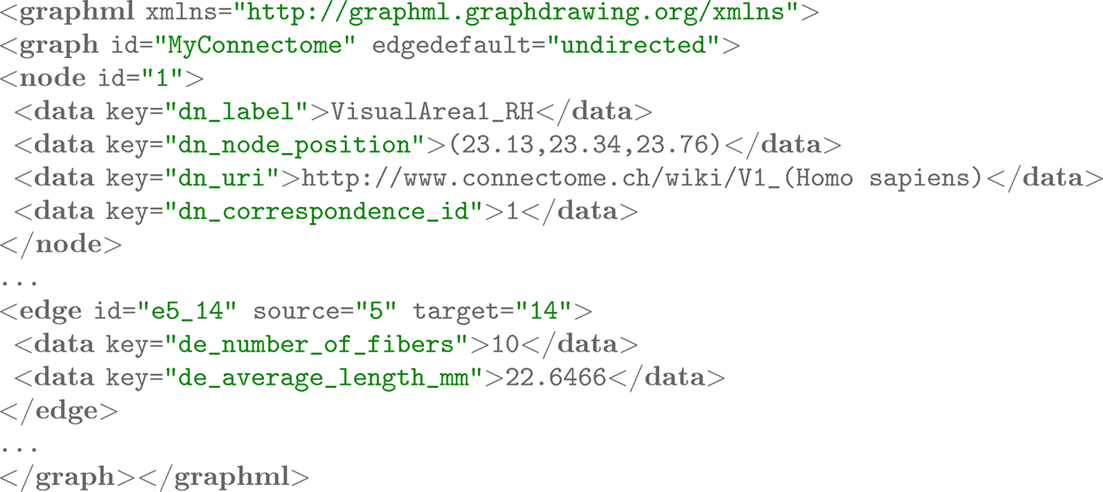
Figure 3. Networks are represented using the GraphML file format. The storage of an arbitrary number of attributes on the nodes and edges is possible. For instance, nodes denoting brain regions may link to semantic frameworks where definitions, delineation criteria, and literature references given. Standardized node positions are useful in graph layouting for comparison.
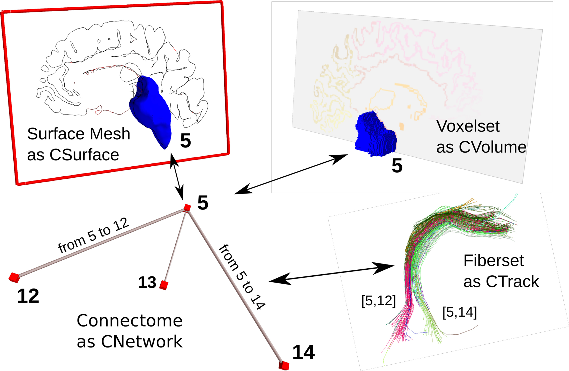
Figure 4. Relationship between multi-modal connectome objects. Correspondence is established with unique (integer) identifiers between the nodes of a network, the ROI in a volumetric dataset, and the surface mesh. Analogically, a network edge has the same identifier as the fiber tracts that connect such two brain regions.
Similarily, this schema is applied to connectivity information, combining the origin and target entities using their unique integer identifiers. The labeling of a subset of fibers of a whole brain tractography corresponds to the group of fibers that connect two brain regions. This connection has its correspondence in an edge of a CNetwork. Additional properties that hold for this group of fibers, such as the number of fibers or averages of scalar values along the fibers, are stored as edge properties. For storing the label information for the fibers belonging to a network edge, we employ a CData object that represents a Nx2 NumPy array. N is the number of fibers and the first row stores integer values denoting the origin region of interest, and the second row stores the target region of interest. As a convention for the undirected fiber data derived from magnetic resonance tractography, we store the smaller integer value always in the first row. Thus, it becomes straightforward to retrieve all the fibers that connect two arbitrary regions of interest for further processing or visualization.
For time-dependent data, the same schema can be used. Time-series data from any source is stored in an NxM dimensional homogenous array. N is the number of channels and M is the number of time points. A CData object contains the labeling for the N channels to relate the series to any entity within the connectome file. Thus, time series can be defined for instance for brain regions, surface patches, network nodes, or electrodes in a very flexible manner. The CTimeseries object is used to store the array, for example in Hierarchical Data Format 5 (HDF512) or NumPy (Oliphant, 2006) array format. In the CTimeseries metadata fields, additional parameters such as the sampling frequency can be stored. Additional CData objects may contain spatial position of the channels.
When psychological assessments are made in clinical trials, the datasets are often stored as spreadsheets. Bundling these data as CData within the connectome files in tabular form (CSV) or as an XML file, facilities data organization, and subsequent statistical correlation procedures with neuroimaging data.
Ultimately, all relevant multi-modal datasets for a neuroimaging study comprising multiple subjects or a single subject can be stored within a single connectome file.
2.2 The Connectome File Format Library
The CFF specification is complemented by the Connectome File Format Library (cfflib) for Python. The cfflib supports (a) reading and writing of the connectome metadata markup (meta.cml) and compressed connectome files, (b) basic Input/Output of the supported file formats using supporting Python libraries, (c) a lazy loading strategy for data, (d) synchronizing files with a remote XNAT database servers, (e) setter and getter methods for updating metadata, (f) auxiliary methods for grouping objects based on metadata tag values and type.
We used the generateDS library (Dave Kuhlmann13) to create the Python object model. All classes were derived from the Connectome File Format XML schema. Subclasses provide additional methods for manipulation of the connectome files and basic loading and saving functionality. An example of an interactive Python session employing cfflib and its object model is given below:
# Import cfflib for usage

   In [1]: import cfflib

   # Load connectome markup file

   In [2]: mycon = cfflib.load(’meta.cml’)

   # Print summary of contained data

   In [3]: mycon.print_ summary()

   # Retrieve particular connectome object by name

   In [4]: mynet = mycon.get_ by_ name(’My
Connectome 83’)

   # Load the connectome data into memory

   In [5]: mynet.load()

   # Display nodes with attributes

   In [6]: print mynet.data.nodes(data = True)

   # On-the-fly grouping based on metadata key-values tags

   In [7]: mygroup = cfflib.group_ by_ tagkey(cobj_

   list = mycon.get_ all(),

   tagkey = "sex", cobj_ type = ["CNetwork"],

   exclude_ values = ["unknown"])

   # Create list of CVolume names

   In [8]: mynamelist = [vol.name for vol in mycon.
get_ connectome_ volume()]
Online tutorials explain extensively how to use cfflib to work with and create new multi-modal connectome files14.
CFF data repository Via our GitHub repository15, we provide a set of public, curated connectome datasets: single subject and group connectome files (generated with the Connectome Mapper), functional connectomes based on fMRI (Biswal et al., 2010), human atlas datasets such as Freesurfer’s fsaverage, MNI152 templates, SRI24 Atlas (Rohlfing et al., 2010), and also some non-human datasets from C. elegans, Macaca Mulatta, and Mouse Brain (Johnson et al., 2010). We welcome contributions of connectome datasets under an open license for this data repository.
Database Interface We support connectome data sharing by providing an interface to remote database infrastructures. The eXtensible Neuroimaging Archive Toolkit (XNAT) is an informatics platform for managing, exploring, and sharing neuroimaging data (Marcus et al., 2007). It exposes web services using a RESTful API. Large neuroimaging initiatives, such as the Human Connectome Project, use the XNAT infrastructure for storage and sharing of large multi-subject, multi-site datasets. The Python library PyXNAT16 interfaces to XNAT servers by their RESTful API. It supports an interactive mode of access for data selection, pulling, and pushing. Any type of data can be pushed to XNAT.
We implemented a push and pull mechanism using PyXNAT for connectome files in cfflib. After the configuration of the connection settings to the XNAT server, it is possible to push and pull connectome files to and from XNAT servers. For pushing the connectome file, the parameters project id, subject id, and experiment id must be set, in order to correctly associate the data in the project organization. All the connectome objects in the container are then submitted to the XNAT server sequentially. For the pulling operation, the same information has to be given with the storage path as an additional parameter. Submitted connectome objects can be displayed and downloaded from the XNAT web interface individually.
2.3 The Connectome Viewer
We wanted to provide neuroimaging researchers with an easy entry into the world of connectome analysis with Python. We designed the Connectome Viewer as a GUI environment with a powerful scripting interface for interactive data analysis and visualization. The primary data source for the application are connectome files. The role of the Connectome Viewer is to provide a tool for the analysis and visualization of connectome files derived from different mapping streams (see Figure 1).
2.3.1 Dependencies
The Connectome Viewer depends on the Enthought Tool Suite (ETS17). ETS provides the application-building framework Envisage and the Traits and Traits UI libraries for creating GUIs. We use Mayavi (Ramachandran and Varoquaux, 2011), the main component in ETS for interactive scientific 3D data visualization, based on the popular Visualization Toolkit VTK (Schröder et al., 2006). Furthermore, we require Chaco for interactive plotting, IPython (Perez and Granger, 2007) for interactive Python shell support and cfflib for data input/output. We rely on the NetworkX (Hagberg et al., 2008) data structures for representation of networks. The dependencies of the Connectome Viewer are listed in Table 2. All required dependencies are installed automatically by using the NeuroDebian repository.
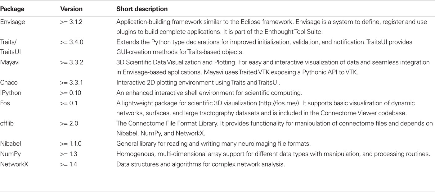
Table 2. Connectome Viewer library dependencies. When using NeuroDebian for the installation, all required dependencies are installed automatically.
2.3.2 Script Generation Mechanism For Usability
The approach we took in the design of the Connectome Viewer to support synergy effects of combined analysis and visualization is based on a simple and proven paradigm. We call it the Code Oracle: for a given task, first a set of graphical user dialogs are presented for the setting of task-relevant parameters. Afterward, a Python script is automatically generated according to the these parameters. Then the script is displayed in the script editor, and can be executed without further modifications in order to perform the requested task. The generated scripts are commented, enabling the researcher to understand the commands performed by the script. It is easily possible to change the basic parameters without going back to the GUI dialogs again by modifying the script directly. Moreover, the commands necessary for reading the appropriate data, performing the visualization and analysis tasks, and generation of results can be modified in the Script Editor.
2.3.3 Plugin Architecture
The Connectome Viewer as an Envisage-based application consists of a set of plugins as the primary building blocks. Plugins may contribute menus, widgets, and other functionality to the application. The core plugins are the Connectome File View, the IPython Shell, the Script Editor, and Mayavi. The Code Oracle and Python Connectome Toolbox are two additional plugins.
The Connectome File View plugin A connectome file can be loaded and saved via the menu. The plugin has a tree view widget that represents the connectome file. All connectome objects are shown in this tree view. Moreover, the loaded connectome file is accessible in the IPython shell for scripting. Double-clicking connectome objects in the tree view loads the referred data file into memory. Connectome objects can be dragged and dropped in the IPython shell for further data inspection and usage in scripts.
The IPython Shell plugin The IPython Shell plugin provides a widget with an enhanced interactive Python shell. Features such as tab-completion, automated docstring display, logging, history, and many others make it an ideal environment for interactive scientific computing.
The Script Editor plugin The Script Editor plugin enables loading, saving, and execution of Python scripts and text files. It features line numbering and syntax highlighting. Scripts can be executed directly in the IPython Shell by keybindings (Ctrl-R for executing or Ctrl-S for saving scripts).
The Mayavi plugin The Mayavi plugin is the major building block that provides advanced interactive 3D visualization and plotting (Ramachandran and Varoquaux, 2011) to the application. It exposes an easy-to-use interface to the well-known Visualization Toolkit VTK (Schröder et al., 2006). Mayavi as a stand-alone application uses the Envisage application framework. Because all functionality is exposed as Envisage plugins, the integration as part of the Connectome Viewer was straightforward. The Mayavi plugin also provides the Mayavi Visualization Tree widget, which manages scenes, visualization objects, and filters hierarchically. Additionally, the Visualization Object Editor lets the user change all parameters of the visualization objects, filters, and scenes.
The Code Oracle plugin We encapsulated the script-generating functionality in the Code Oracle plugin. The Code Oracle plugin adds a menu to the Connectome Viewer for invoking the Code Oracle mechanism for specific task. The Code Oracle menu is structured according to analysis and visulization task on the different connectome file objects: “Surface Mesh With Labels” (CSurface); “Volume Slicer,” “Volume Rendering” (CVolume); “Network Visualization,” “Connection Matrix Viewer,” “Network Report” (CNetwork); “Network-based statistic (NBS)” (Statistics); “Fiber Visualization” (CTrack); “XNAT Push and Pull” (Other); “Brain Extraction using BET” (Nipype).
This list presents a set of basic functionality. Several generated Code Oracle scripts may be combined and modified in the script editor for more complex tasks. The number of generated scripts is expected to grow rapidly as new use cases are discovered and algorithms developed and integrated.
The Python Connectome Toolbox plugin The Python Connectome Toolbox serves as a container for a collection of connectome-related analysis algorithms. They can also be used without the GUI. We provide within the Python Connectome Toolbox a Python wrapper to the C++ implementation bct-cpp (Williams et al., 2011) of the Brain Connectivity Toolbox (Rubinov and Sporns, 2009). We expose all of the toolbox’s functions with an easy-to-use interface and parameter descriptions. The Brain Connectivity Toolbox algorithms are widely used for network analysis in the neuroimaging community. An abundance of additional well-designed network analysis libraries and Python wrappers exist that cover almost all aspects of network-based connectome analysis: NetworkX (Hagberg et al., 2008), Boost Graph Library (Siek et al., 2001), iGraph (Csardi and Nepusz, 2006), graph-tool18, or Python-graph19.
Furthermore, we provide within the toolbox two Network-based statistics for case–control or task-control group studies: the Network-based statistic (Zalesky et al., 2010) and Block-based statistic (Meskaldji et al., 2010). The Code Oracle plugin produces scripts that use the Python Connectome Toolbox’s functionality.
2.3.4 Supporting Libraries
Through the open design of the Connectome Viewer, we encourage the use of the many libraries available in the scientific Python community. The supporting libraries presented here provide powerful tools for creative data exploration and data mining. Every library is usable from the IPython widget in the Connectome Viewer. Vice versa, contributed packages to the Connectome Viewer are usable from a pure IPython shell if they do not require the GUI.
The Neuroimaging in Python (NIPY20) project (Millman and Brett, 2007) is an umbrella project for various efforts to build well-written and documented open source neuroimaging libraries. Currently, NIPY consists of the following five packages. A few more helpful packages for the neuroimaging researcher have been added to the list:
Nibabel “Nibabel provides read and write access to some common medical and neuroimaging file formats, including: ANALYZE, GIFTI, NIfTI1, MINC, DICOM, MGH, TrackVis, as well as PAR/REC.” Nibabel constitutes a necessary component for writing data analysis workflows, because it is crucial to retrieve and exchange data across different analysis software and computer platforms.
Dipy “Dipy is an international, free and open software project for diffusion magnetic resonance imaging analysis in Python. DiPy includes methods for reconstruction, resampling, tractography, warping, fiber clustering and visualization.” (Garyfallidis et al., 2011)
Nipype “Nipype, an open source, community-developed initiative under the umbrella of NIPY, is a Python project that provides a uniform interface to existing neuroimaging software and facilitates interaction between these packages within a single workflow. Nipype provides an environment that encourages interactive exploration of algorithms from different packages, eases the design of workflows within and between packages, and reduces the learning curve necessary to use different packages.” (Ghosh et al., 2010)
Nitime “Nitime is a library for time-series analysis of data from neuroscience experiments. It contains a core of numerical algorithms for time-series analysis both in the time and spectral domains, a set of container objects to represent time-series, and auxiliary objects that expose a high-level interface to the numerical machinery and make common analysis tasks easy to express with compact and semantically clear code.” (Rokem et al., 2009)
NiPy “NiPy is a Python-based framework for the analysis of structural and functional neuroimaging data. It currently has a full system for general linear modeling of functional magnetic resonance imaging (fMRI).”
PyROI “PyROI is a Python package for functional neuroimaging region of interest extraction and analysis. It offers an efficient processing stream and a wide range of flexibility in the way source images are parcellated. Using PyROI, users can extract parameter and contrast effect sizes or timecourses.”21
PyMVPA “PyMVPA is a Python package intended to ease statistical learning analyses of large datasets. It offers an extensible framework with a high-level interface to a broad range of algorithms for classification, regression, feature selection, data import and export. While it is not limited to the neuroimaging domain, it is eminently suited for such datasets.” (Hanke et al., 2009)
scikit-learn “For easy-to-use and general-purpose machine learning in Python. It contains supervised learning (SVM, GLM), as well as unsupervised learning algorithms.”22
We want to emphasize the additional tremendous potential for data exploration and data mining of connectomes using these external libraries. For a functional mapping stream, PyROI may be used to extract averaged time series from regions of interest. Nitime may then be used to perform functional connectivity analysis from extracted time-series data. Nipype is ready to implement even more sophisticated data workflows using external packages and parallelize them on cluster infrastructures. For Diffusion MRI, Dipy implements reconstruction, tractography, and fiber visualization methods in a free and open source manner. Furthermore, the PyMVPA framework and the scikit-learn library provide widely used machine learning algorithms. The application of machine learning methods is facilitated for non-experts through extensive online tutorials, for instance in tutorials on fMRI decoding analysis with scikit-learn23 or a general introduction to the PyMVPA framework24.
2.4 Connectome Mapping Workflows
The general workflow to derive useful connectome information from primary neuroimaging data was shown in Figure 1. Data used here for the demonstration of the Connectome Viewer Toolkit is derived from Diffusion MRI. We reimplemented the pipeline used by Hagmann et al. (2008). We used the Traits and Traits UI libraries to build a GUI for the Connectome Mapper tool. The Connectome Mapper’s processing stages are depicted Figure 5. All image processing stages can be parameterized and run interactively, or remotely using a configuration script. Details of the individual processing stages are available from the online documentation. The Connectome Mapper is released together with the Connectome Viewer Toolkit as the Connectome Mapping Toolkit25, but the toolkit can be used as stand-alone application, and also with other mapping workflows, such as Nipype.

Figure 5. The general processing stages of the Connectome Mapper. This pipeline is an example implementation of a structural connectome mapping stream. Here, two processing streams dealing separately with brain region (node) and white matter (edge) information eventually converge into the connectome of one particular subject.
We will not detail the Connectome Mapper architecture, individual processing stages or validation issues here. We note only that the last “Connectome Creation” stage merges data from the two processing streams. The fibers from tractography are merged with volumetric region of interest masks denoting brain regions to form a network. This step exemplifies one instance of establishing the relationships between multi-modal data types as shown in Figure 4.
The multi-modal datasets produced by connectome worksflows was a major motivation to create the CFF. The product of such a mapping stream not only comprises the resulting connection matrix, but also fibers, surfaces, segmentations, labelings, other data arrays, and metadata. Capturing provenance information and storing it along with the raw and processed data is very important for later reproducibility. There are no accepted standards in the neuroimaging community for provenance tracking. In the Connectome Mapper, the log and configuration file including versions of the called executables and the operating system environment are stored for provenance everytime the pipeline is run. The CFF provides a convenient way to store this data, as well as other provenance information.
3 Results
Connectome file for Multi-Modal Datasets The last processing stage of the Connectome Mapper implements an automatic conversion of original and processed data into connectome files. Using cfflib, data with relevance for subsequent analysis and visualization are packed into a connectome file. In the Connectome Mapper, the generated connectome files usually consist of the networks (CNetwork), the volumetric segmentations and the raw data (CVolume), the extracted surfaces with their brain region labeling (CSurfce), the original and filtered fibers from the deterministic tractography (CTrack), the fiber labeling and property arrays (CData), and the subject and project metadata (CMetadata). During the pipeline configuration, these subject- and project-specific metadata fields have to be entered. In a postprocessing step, additional datasets such as psychological assessment and behavioral assays can be added to the generated connectome file.
An excerpt of the connectome markup meta.cml for a single subject that was generated in the conversion stage of the processing pipeline is shown in Figure 6. It is enriched by an example section that contains information about the EEG acquisition parameters.
The connectome file may now be published to a public or private repository or database infrastructure. For instance, the connectome file can be published to an XNAT server (Marcus et al.,2007) using cfflib and PyXNAT with a few lines of Python code. The required commands are generated with the “XNAT Push and Pull” function of the Code Oracle plugin. For further analysis and visualization, the connectome file is loaded in the Connectome Viewer. The Connectome File View widget is updated and may appear as in Figure 7, displaying nodes for each connectome object in the connectome file.
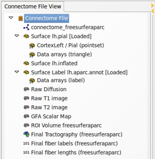
Figure 7. Connectome File View as a Connectome Viewer widget. The treeview gives a convenient user interface to deal with connectome objects contained in a connectome file. Data files are loaded into memory by double-clicking. Single tree nodes can be dragged to the IPython shell for data inspection and scripting.
The Connectome Viewer GUI consists of widgets contributed by its core plugins. The main window after loading a connectome file and executing a surface display script (using the Code Oracle) with an anatomical cortical parcellation (Desikan et al., 2006) is shown in Figure 8.
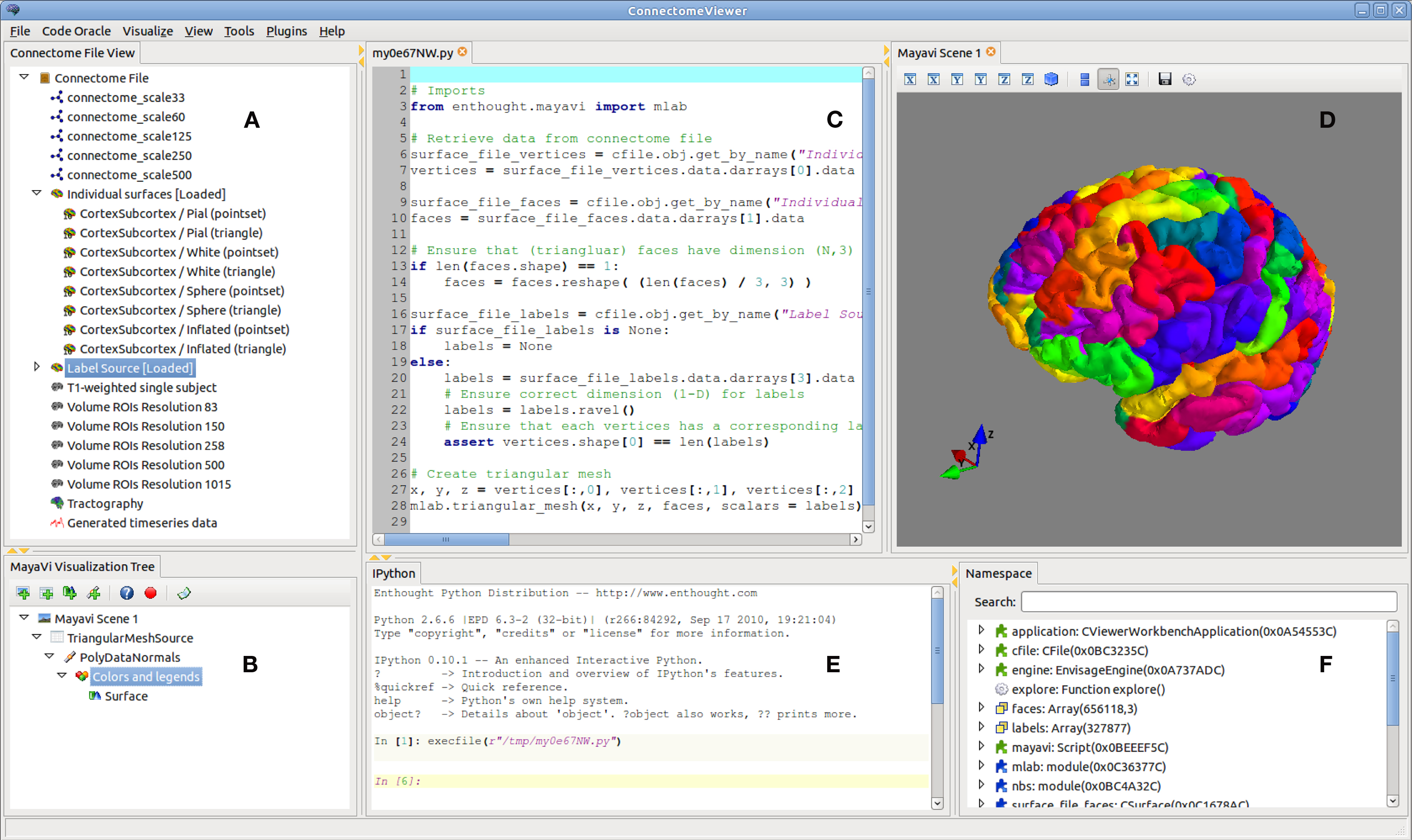
Figure 8. The Connectome Viewer GUI. The main application is shown with the placeable widgets contributed by the core plugins. (A) The Connectome File View shows a treeview of the contents of a loaded connectome file. (B) The Mayavi Visualization Tree manages the visualization objects and scenes in a pipeline. (C) The ScriptEditor shows scripts generated with the Code Oracle with syntax highlighting. They can be manipulated and run in the IPython console. (D) The Mayavi Scene displays the visualized data. (E) The IPython shell is integrated as a widget. It exposes the loaded connectome file and other objects for interactive scripting and data inspection. (F) The Namespace widget displays the variables and packages currently loaded in memory and accessible in the IPython Shell.
In Figure 9, the connectivity matrix based on particular Diffusion-derived measures for edge values is presented in an interactive user interface. The interface allows the user to zoom, drag, select the display range, switch between different edge values, and show the connecting regions when moving over an edge.

Figure 9. Node degree display on the surface of an inflated left hemisphere (left). The right hemisphere and parts of the medial surface of the left hemisphere are clipped using the Mayavi DataSet Clipper. A set of left hemispheric cortical and subcortical regions is visible. The node degree of each region is coded in color. Blue corresponds to a low degree, green to a medium degree, and red to a high degree. The Connection Matrix Viewer (right). Switching between edge values and highlighting of the edge value ranges is possible. The From and To labels, and edge values are updated automatically when moving over the matrix with the mouse cursor.
An instance of multi-modal data integration using network properties and reconstructed surfaces is depicted in Figure 9. A simple network metric, namely the node degree (number of adjoining edges), was computed. The nodes correspond to brain regions, delineated on a inflated brain surface. The node degree values were then used for color-coding the corresponding regions. Mayavi provides the DataSet Clipper to clip the surface mesh and reveal the view onto the subcortical nuclei. Comparatively, a much higher node degree is readily recognizable for the subcortical regions compared to the low node degree on the cortical surface.
The results of a Code Oracle analysis script to extract and cluster cortico-cortico U-fibers from tractography are shown in Figure 10. It uses supporting Python libraries, such as NumPy for array handling and comparison, Dipy for the local skeleton clustering algorithm (Garyfallidis et al., 2010) and Fos for visualization. Interactively, improvements in the fiber extraction and clustering parameters were made. The direct influence of parameter changes in the script are readily visible by re-executing the script. The script “U-fiber Extraction” to reproduce Figure 10 can be invoked from the Code Oracle plugin.
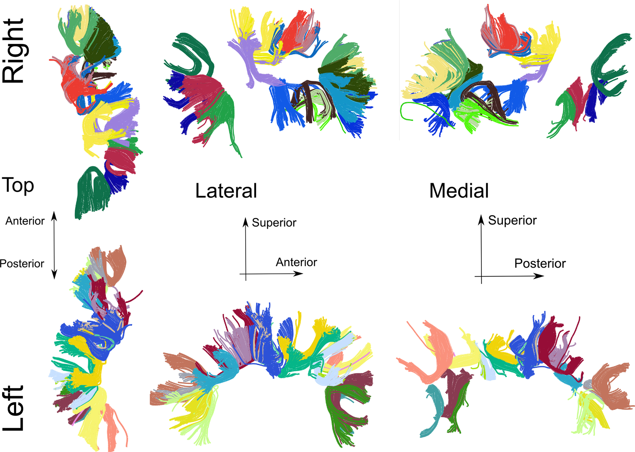
Figure 10. Cortico-cortico U-shaped fibers generated with a Code Oracle script. The method to extract fibers from a subject uses criteria for fiber start and endpoint closeness, fiber curvature. The local skeleton clustering procedure (Garyfallidis et al., 2011) is used for the cluster coloring. The extracted U-fibers are cortical short distance connections hypothesized to contribute to the cortical small world network property (Bassett and Bullmore, 2006).
Furthermore, we show an example PDF output of the network report generation mechanism, created using the “Network Report” Code Oracle (Figure 11). For PDF creation, ReportLab26 is used. The figures in the report are generated using Matplotlib (Hunter, 2007) for 2D plotting. Connection matrix and node degree histograms are displayed along with basic network statistics for a selected networks contained in the currently loaded connectome file. The script that produces the reports can easily be adapted for modification of the layout or report content to include other network measures or visualizations (Figure 12).
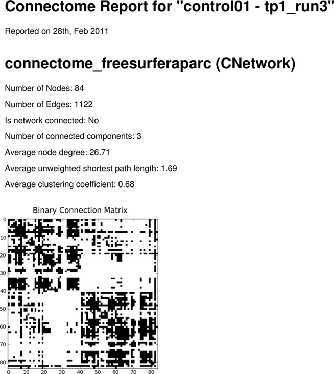
Figure 11. Network PDF Report. Reports can be automatically generated using the Code Oracle “Network Report.” The layout and report content can be adapted and extended with required results.
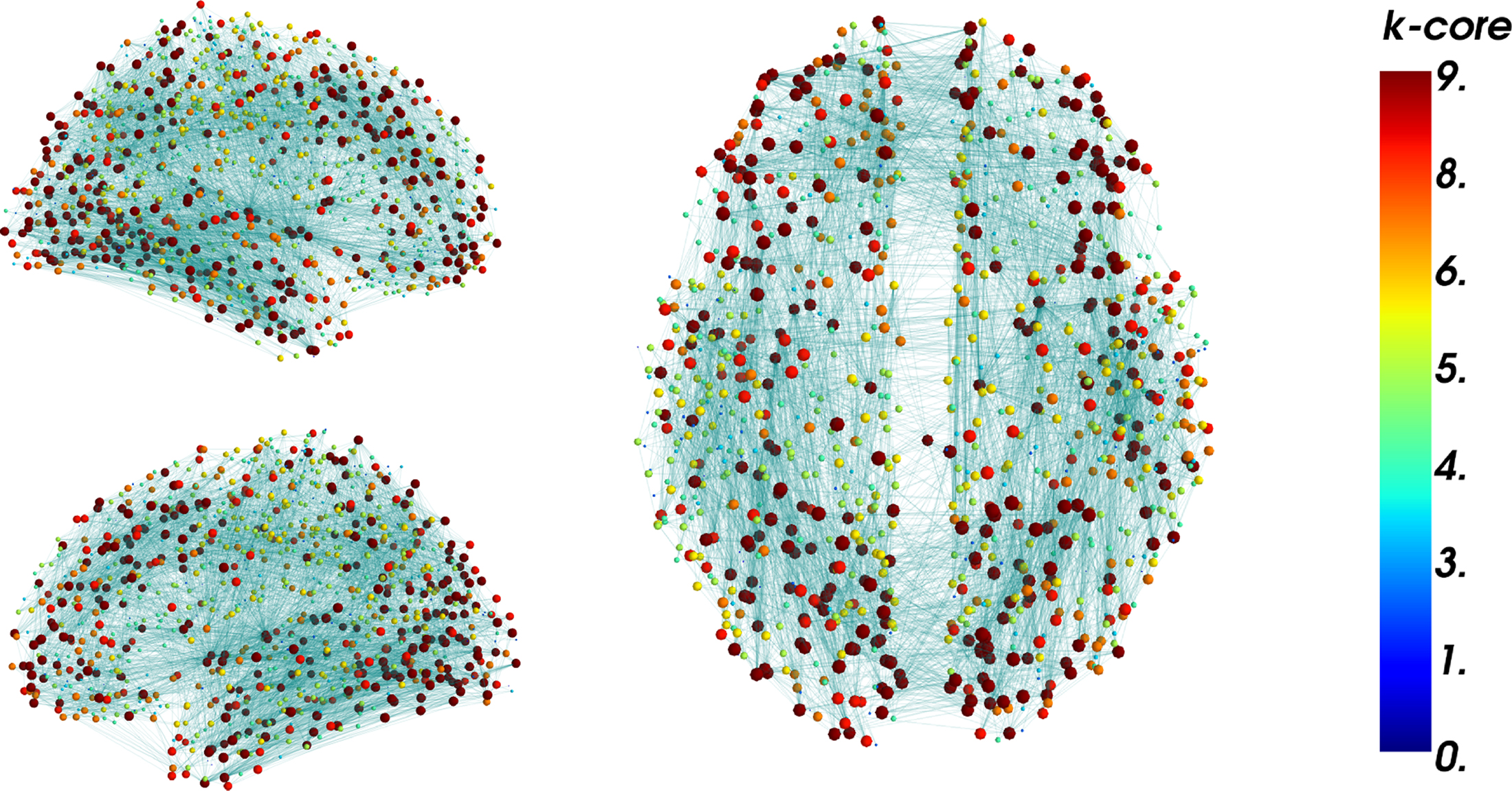
Figure 12. Brain Connectivity Hairball. Display of the whole connectivity information at once does not allow for any sensible interpretation. Interactive manipulation of visualization parameters such as node position and coloring enables data exploration. Nodes are located here at the center of gravity of their underlying inflated brain region mesh. Nodes are scaled and colored according to their k-core number. The k-core number was computed using NetworkX in the IPython shell. The numbers were reused as a parameter to update the visualization interactively. Segregation of nodes with high k-core number at particular regions may be visible (Hagmann et al., 2008).
4 Discussion
4.1 Connectome File Format
In this article, we exemplified the application of the CFF for Diffusion MRI data and metadata. We envision more use cases of functional connectivity analysis using fMRI, EEG, MEG methods. The CFF specification is flexible enough to also accommodate such multi-modal datasets and their metadata.
One current limitation is a missing specification in the format itself of the shared spatial data space among connectome object types. For instance, it is possible that the affine transformation stored in NIFTI or GIFTI files do not map to the same common space, such as MNI152, due to different preprocessing. The annotation of the particular data spaces for individual connectome objects as metadata of the connectome file is possible.
As multi-modal or multi-subject datasets are often very large, in the order of tens or hundreds of gigabytes, having all datasets in one compressed container is disadvantageous for fast file access and manipulation. Because the meta.cml file stores relative references to the connectome object data files, the data files can reside on the local or remote file system in subfolders relative to the meta.cml file. The meta.cml can be loaded with cfflib, thereby exposing the all contained connectome objects. This enables fast access and manipulation of the connectome objects without decompression and compression steps. Existing compression mechanisms for individual data files such as GZIP for NIFTI and GIFTI files reduce the data size substantially and can still be employed. Only for data exchange or distribution, the multi-modal dataset is ZIP compressed (filename ending.cff). We adopted the ZIP compression algorithm because it is widely supported and gives good performance in terms of fast compression and compression ratio on medium-sized datasets, such as single subject datasets.
The XML-Based Clinical Experiment Data Exchange Schema XCEDE2 (Gadde et al., 2011) provides an extensive metadata hierarchy for experimental context representation, provenance, and protocol information. Whereas XCEDE2 focuses on complete representation of neuroimaging studies and uses web frontends for data manipulation and annotation, the CFF metadata hierarchy is more open, flexible, and analysis-centric. All CFF data manipulation can be performed using cfflib from an interactive Python console. Experimental context representation may be stored as CData objects. For example, they may contain instances of XCEDE2 files.
The CIFTI format for connectivity-related neuroimaging data is proposed by the CIFTI and is based on the NIFTI-2 format. Currently, we employ GraphML to store connectivity graphs and associate them with surface and volume-based datasets, but adopting the CIFTI format for this purpose will be rather straightforward.
Recently, efforts to standardize terminologies and build ontologies for neuroscience have undergone a resurgence (Larson and Martone, 2009). We encourage linking to and referencing existing ontologies as much as possible. For instance, every node in a network produced by the Connectome Mapper denotes a brain structure. With attributes on these nodes, we refer to a unique Uniform Resource Identifier, as seen in Figure 3, pointing to a standardized ontology or wiki. This reference allows other researchers to retrieve the concept and delineation criteria for a particular brain structure in a parcellation scheme. In addition, the annotation of metadata by the researcher, together with using standardized terminologies, will facilitate future data integration challenges of connectome datasets.
4.2 Connectome File Format Library
We used the CFF object model to create the Python library cfflib for connectome file manipulation and annotation. Within the Connectome Viewer Toolkit, cfflib naturally serves to convert multi-modal datasets and metadata from the Connectome Mapper into a connectome file. The Connectome Viewer uses cfflib to load and save connectome files. Thus, the CFF and cfflib serve well as interfacing tools.
As new file format input/ouput libraries are developed, the cfflib will be able to reuse these libraries to expose a common interface to the neuroimaging researcher dealing with multi-modal datasets of different file formats.
4.3 Connectome Viewer
We have demonstrated the usability of the Connectome Viewer as a research and development environment. Our experience has shown that integrating analysis, data manipulation, and visualization capabilities synergistically in a single application is beneficial to researchers. This is especially true for data exploration and data mining. Extending visualization applications with analysis and data manipulation functionality by including a Python shell was recently achieved in 3D Slicer (Gering et al., 2001). 3D Slicer is a comprehensive application for multi-modal visualization with over one million lines of mostly C++ code. The underlying toolkit for visualization is VTK. By using Mayavi as an interface to VTK, we can hide much of the complexity of VTK and provide an easy-to-use interface for visualization to the researcher. Mayavi provides extensive documentation and examples for many use cases, yet it allows one to use the underlying VTK objects if necessary. Similarily, the DataViewer3D (Gouws et al., 2009) uses VTK directly to provide multi-modal visualization capabilities and is Python-based. DataViewer3D does not include a Python shell for analysis and does not use the Enthought Toolsuite or Mayavi.
We have reused supporting libraries as much as possible, taking advantage from the expertise of library developers in their various domains. This has led to a comparatively small codebase for the Connectome Viewer which is approachable for contributor who may wish to create extensions. The modular plugin architecture furthers this. Through the Code Oracle script generation mechanism, the Connectome Viewer facilitates the introduction to Python scripting considerably. The scripts are easily adaptable and extendable to the needs of connectome researcher. As our experience shows, writing Python scripts feels very familiar to researchers used to other development environments such as Matlab, and can be learned in a short time period.
5 Conclusion
We have proposed the Connectome File Format as a convenient, easy-to-use container data format to deal with some of the heterogeneity and complexity of multi-modal neuroimaging data. The CFF connects multi-modal data sources and metadata in a comprehensive and flexible way. We have showed how the CFF and its accompanying Python library cfflib solve data management and integration challenges. We also foresee the usefulness of the CFF for datasets from functional neuroimaging and behavioral domains.
We have presented the Connectome Viewer, an integrated neuroinformatics research and development framework for 3D visualization and analysis. The modular plugin architecture provides means for extensibility and the Code Oracle method supports leveraging of the scripting interface by an automated script generation mechanism for common analysis tasks. The full compatibility with the CFF facilitates cross-modal data mining, analysis and visualization in an interactive, scriptable way.
The Connectome Viewer Toolkit, its supporting libraries and the Connectome Mapper constitute the Connectome Mapping Toolkit. Altogether, this toolkit creates a unique, extensible workbench for new and ongoing macroscale connectome mapping, management, analysis, and visualization.
6 Information Sharing Statement
The Connectome Viewer Toolkit is released under the terms of the open source Modified BSD license (opensource.org/licenses/bsd-license.php). Contributed packages and plugins adhere to their own open source licensing policy. All packages, documentation and example datasets can be downloaded from http://www.cmtk.org/. Furthermore, the tools are listed and associated in the Neuroimaging Informatics Tools and Resources Clearinghouse under http://www.nitrc.org/.
Conflict of Interest Statement
The authors declare that the research was conducted in the absence of any commercial or financial relationships that could be construed as a potential conflict of interest.
Acknowledgments
We would like to thank the NIPY community and the open source Python community in general. Special thanks go to Leila Cammoun, Gaël Varoquaux for Mayavi development and support, Yannick Schwartz for PyXNAT, Eleftherios Garyfallidis for the Dipy package and the Fos vision, Christophe Chênes for supporting the development of cfflib, Erik Ziegler for the Nipype connectivity tutorial, and Mark Longair, Patricia Milz, and Alessandra Griffa for their helpful comments on the manuscript. This work is partially supported by the SPUM project number 33CM30-124089 of the Swiss National Science Foundation.
Footnotes
- ^www.python.org
- ^humanconnectome.org
- ^nifti.nimh.nih.gov
- ^www.nitrc.org/frs/? group_id = 75
- ^www.incf.org/core/programs/datasharing
- ^github.com/LTS5
- ^sphinx.pocoo.org
- ^neuro.debian.net
- ^www.enthought.com
- ^http://www.g-node.org/projects/odml
- ^graphml.graphdrawing.org
- ^www.hdfgroup.org
- ^www.rexx.com/?dkuhlman/generateDS.html
- ^cmtk.org/cfflib/
- ^github.com/LTS5/cffdata
- ^packages.python.org/pyxnat/
- ^code.enthought.com
- ^projects.skewed.de/graph-tool/
- ^code.google.com/p/python-graph/
- ^nipy.org
- ^web.mit.edu/mwaskom/pyroi/
- ^scikit-learn.sourceforge.net
- ^nisl.github.com/
- ^www.pymvpa.org/tutorial.html
- ^www.cmtk.org
- ^reportlab.com
References
Akil, H., Martone, M. E., and Van Essen, D. C. (2011). Challenges and opportunities in mining neuroscience data. Science 331, 708–712.
Anderson, J., Jones, B., Watt, C., Shaw, M., Yang, J.-H., DeMill, D., Lauritzen, J., Lin, Y., Rapp, K., Mastronarde, D., Koshevoy, P., Grimm, B., Tasdizen, T., Whitaker, R., and Marc, R. (2011). Exploring the retinal connectome. Mol. Vis. 17, 355–379.
Baxter, S. M., Day, S. W., Fetrow, J. S., and Reisinger, S. J. (2006). Scientific software development is not an oxymoron. PLoS Comput. Biol. 2, e87.
Benger, W. (2009). On safari in the file format jungle – why can’t you visualize my data? Comput. Sci. Eng. 11, 98–102.
Binzegger, T., Douglas, R. J., and Martin, K. A. C. (2004). A quantitative map of the circuit of cat primary visual cortex. J. Neurosci. 24, 8441–8453.
Biswal, B. B., Mennes, M., Zuo, X. N., Gohel, S., Kelly, C., Smith, S. M., Beckmann, C. F., Adelstein, J. S., Buckner, R. L., Colcombe, S., Dogonowski, A. M., Ernst, M., Fair, D., Hampson, M., Hoptman, M. J., Hyde, J. S., Kiviniemi, V. J., Kötter, R., Li, S. J., Lin, C. P., Lowe, M. J., Mackay, C., Madden, D. J., Madsen, K. H., Margulies, D. S., Mayberg, H. S., McMahon, K., Monk, C. S., Mostofsky, S. H., Nagel, B. J., Pekar, J. J., Peltier, S. J., Petersen, S. E., Riedl, V., Rombouts, S. A., Rypma, B., Schlaggar, B. L., Schmidt, S., Seidler, R. D., Siegle, G. J., Sorg, C., Teng, G. J., Veijola, J., Villringer, A., Walter, M., Wang, L., Weng, X. C., Whitfield-Gabrieli, S., Williamson, P., Windischberger, C., Zang, Y. F., Zhang, H. Y., Castellanos, F. X., and Milham, M. P. (2010). Toward discovery science of human brain function. Proc. Natl. Acad. Sci. U.S.A. 107, 4734–4739.
Bullmore, E., and Sporns, O. (2009). Complex brain networks: graph theoretical analysis of structural and functional systems. Nat. Rev. Neurosci. 10, 186–198.
Cardona, A., Saalfeld, S., Preibisch, S., Schmid, B., Cheng, A., Pulokas, J., Tomancak, P., and Hartenstein, V. (2010). An integrated micro- and macroarchitectural analysis of the Drosophila brain by computer-assisted serial section electron microscopy. PLoS Biol. 8, e1000502. doi: 10.1371/journal.pbio.1000502
Chacon, S. (2009). Pro Git. Apress, 288. Available at: http://progit.org/book/
Chklovskii, D. B., Vitaladevuni, S., and Scheffer, L. K. (2010). Semi-automated reconstruction of neural circuits using electron microscopy. Curr. Opin. Neurobiol. 20, 8.
Csardi, G., and Nepusz, T. (2006). The igraph software package for complex network research. InterJournal Complex Syst. 1695.
Davison, A. P., Hines, M. L., and Muller, E. (2009). Trends in programming languages for neuroscience simulations.e87. Front. Neurosci. 3:374–80. doi: 10.3389/neuro.01.036.2009
Desikan, R. S., Ségonne, F., Fischl, B., Quinn, B. T., Dickerson, B. C., Blacker, D., Buckner, R. L., Dale, A. M., Maguire, R. P., Hyman, B. T., Albert, M. S., and Killiany, R. J. (2006). An automated labeling system for subdividing the human cerebral cortex on MRI scans into gyral based regions of interest. Neuroimage 31, 968–80.
Douglas, R. J., and Martin, K. A. C. (2007). Mapping the matrix: the ways of neocortex. Neuron 56, 226–238.
Felleman, D. J., and Van Essen, D. C. (1991). Distributed hierarchical processing in the primate cerebral cortex. Cereb. Cortex 1, 1–47.
Gadde, S., Aucoin, N., Grethe, J. S., Keator, D. B., Marcus, D. S., and Pieper, S. (2011). XCEDE: an extensible schema for biomedical data. Neuroinformatics 1–14.
Garyfallidis, E., Brett, M., Amirbekian, B., Nguyen, C., Yeh, F.-C., Halchenko, Y., and Nimmo-Smith, I. (2011). “Dipy – a novel software library for diffusion MR and tractography,” in 17th Annual Meeting of the Organization for Human Brain Mapping, Quebec (submitted).
Garyfallidis, E., Brett, M., and Nimmo-Smith, I. (2010). “Fast dimensionality reduction for brain tractography clustering,” in 16th Annual Meeting of the Organization for Human Brain Mapping, Barcelona.
Gering, D. T., Nabavi, A., Kikinis, R., Hata, N., O’Donnell, L. J., Grimson, W. E., Jolesz, F. A., Black, P. M., and Wells, W. M. (2001). An integrated visualization system for surgical planning and guidance using image fusion and an open MR. J. Magn. Reson. Imaging 13, 967–975.
Ghosh, S., Burns, C., Clark, D., Gorgolewski, K., Halchenko, Y., Madison, C., Tungaraza, R., and Millman, K. (2010). “Nipype: opensource platform for unified and replicable interaction with existing neuroimaging tools,” in 16th Annual Meeting of the Organization for Human Brain Mapping, Barcelona.
Gouws, A., Woods, W., Millman, R., Morland, A., and Green, G. (2009). DataViewer3D: an open-source, cross-platform multi-modal neuroimaging data visualization tool. Front. Neuroinformatics 3:9. doi: 10.3389/neuro.11.009.2009
Hagberg, A. A., Schult, D. A., and Swart, P. J. (2008). “Exploring network structure, dynamics, and function using NetworkX,” in Proceedings of the 7th Python in Science Conference, eds G. Varoquaux, T. Vaught, and J. Millman (Pasadena, CA).
Hagmann, P. (2005). From Diffusion MRI to Brain Connectomics. PhD thesis, Ecole Polytechnique Fédérale de Lausanne, Lausanne, 127.
Hagmann, P., Cammoun, L., Gigandet, X., Meuli, R., Honey, C. J., Wedeen, V. J., and Sporns, O. (2008). Mapping the structural core of human cerebral cortex. PLoS Biol. 6, e159. doi: 10.1371/journal.pbio.0060159
Hagmann, P., Cammoun, L., Gigandet, X., Gerhard, S., Ellen Grant, P., Wedeen, V., Meuli, R., Thiran, J.-P., Honey, C. J., and Sporns, O. (2010). MR connectomics: principles and challenges. J. Neurosci. Methods 194, 34–45.
Hampel, S., Chung, P., McKellar, C. E., Hall, D., Looger, L. L., and Simpson, J. H. (2011). Drosophila brainbow: a recombinase-based fluorescence labeling technique to subdivide neural expression patterns. Nat. Methods 8, 253–259.
Hanke, M., Halchenko, Y. O., Sederberg, P. B., Olivetti, E., Fründ, I., Rieger, J. W., Herrmann, C. S., Haxby, J. V., Hanson, S. J., and Pollmann, S. (2009). PyMVPA: a unifying approach to the analysis of neuroscientific data. Front. Neuroinformatics 3:3. doi: 10.3389/neuro.11.003.2009.
Johansen-Berg, H., and Behrens, T. E. J. (2009). Diffusion MRI: From Quantitative Measurement to In-vivo Neuroanatomy. London: Academic Press, 490.
Johnson, G. A., Badea, A., Brandenburg, J., Cofer, G., Fubara, B., Liu, S., and Nissanov, J. (2010). Waxholm space: an image-based reference for coordinating mouse brain research. Neuroimage 53, 365–372.
Langtangen, H. P. (2009). A Primer on Scientific Programming with Python (Texts in Computational Science and Engineering). New York: Springer, 693.
Larson, S. D., and Martone, M. E. (2009). Ontologies for neuroscience: what are they and what are they good for? Front. Neurosci. 3:1. doi: 10.3389/neuro.01.007.2009
Lu, J., Tapia, J. C., White, O. L., and Lichtman, J. W. (2009). The interscutularis muscle connectome. PLoS Biol. 7, e32. doi: 10.1371/journal. pbio.1000032.
Macagno, E. R., Levinthal, C., and Sobel, I. (1979). Three-dimensional computer reconstruction of neurons and neuronal assemblies. Annu. Rev. Biophys. Bioeng. 8, 323–351.
Marcus, D. S., Olsen, T. R., Ramaratnam, M., and Buckner, R. L. (2007). The Extensible Neuroimaging Archive Toolkit: an informatics platform for managing, exploring, and sharing neuroimaging data. Neuroinformatics 5, 11–34.
Markov, N. T., Misery, P., Falchier, A., Lamy, C., Vezoli, J., Quilodran, R., Gariel, M. A., Giroud, P., Ercsey-Ravasz, M., Pilaz, L. J., Huissoud, C., Barone, P., Dehay, C., Toroczkai, Z., Van Essen, D. C., Kennedy, H., and Knoblauch, K. (2010). Weight consistency specifies regularities of macaque cortical networks. Cereb. Cortex 21, 1254–1272.
Meskaldji, D. E., Cammoun, L., Hagmann, P., Meuli, R., Thiran, J. P., and Morgenthaler, S. (2010). Efficient statistical analysis of large correlated multivariate datasets: a case study on brain connectivity matrices. Available at: http://arxiv.org/abs/1008.1909.
Millman, K. J., and Brett, M. (2007). Analysis of functional magnetic resonance imaging in Python. Comput. Sci. Eng. 9, 52–55.
Oliphant, T. E. (2006). Guide to NumPy. Trelgol Publishing. Available at: http://www.tramy.us/
Perez, F., and Granger, B. E. (2007). IPython: a system for interactive scientific computing. Comput. Sci. Eng. 9, 21–29.
Ramachandran, P., and Varoquaux, G. (2011). Mayavi: a package for 3D visualization of scientific data. Comput. Sci. Eng. 13, 40.
Rohlfing, T., Zahr, N. M., Sullivan, E. V., and Pfefferbaum, A. (2010). The SRI24 multichannel atlas of normal adult human brain structure. Hum. Brain Mapp. 31, 798–819.
Rokem, A., Trumpis, M., and Perez, F. (2009). “Nitime: time-series analysis for neuroimaging data,” in Proceedings of the 8th Python in Science conference, eds. G. Varoquaux, S. Van Der Walt, and J. Millman Pasadena, CA, 68–75.
Rubinov, M., and Sporns, O. (2009). Complex network measures of brain connectivity: uses and interpretations. Neuroimage 52, 1059–1069.
Schröder, W., Martin, K., and Lorensen, B. (2006). Visualization Toolkit: An Object-Oriented Approach to 3D Graphics, 4th Edn. Kitware Inc: New York 528.
Siek, J. G., Lee, L.-Q., and Lumsdaine, A. (2001). The Boost Graph Library: User Guide and Reference Manual. Boston, MA: Addison-Wesley Professional, 352.
Spacek, M., Blanche, T., and Swindale, N. (2008). Python for large-scale electrophysiology. Front. Neuroinformatics 2:9. doi: 10.3389/neuro.11.009.2008
Sporns, O., Tononi, G., and Kötter, R. (2005). The human connectome: a structural description of the human brain. PLoS Comput. Biol. 1, e42. doi: 10.1371/journal.pcbi.0010042
Thompson, H. S., Beech, D., Maloney, M., and Mendelsohn, N. (2004). XML Schema Part 1: Structures, 2nd Edn. W3C Recommendation. Available at: http://www.w3.org/TR/xmlschema-1/
Ward, S., Thomson, N., White, J. G., and Brenner, S. (1975). Electron microscopical reconstruction of the anterior sensory anatomy of the nematode Caenorhabditis elegans. J. Comp. Neurol. 160, 313–37. doi: 10.1002/cne.901600305
Wedeen, V. J., Wang, R. P., Schmahmann, J. D., Benner, T., Tseng, W. Y. I., Dai, G., Pandya, D. N., Hagmann, P., D’Arceuil, H., and de Crespigny, A. J. (2008). Diffusion spectrum magnetic resonance imaging (DSI) tractography of crossing fibers. Neuroimage 41, 1267–1277.
White, J. G., Southgate, E., Thomson, J. N., and Brenner, S. (1976). The structure of the ventral nerve cord of Caenorhabditis elegans. Philos. Trans. R. Soc. Lond. B Biol. Sci. 275, 327–348.
Williams, S., Manicka, S., and Yaeger, L. (2011). bct-cpp. Available at: http://code.google.com/p/bct-cpp/
Keywords: connectomics, connectome, neuroimaging, python, multi-modal data, data management, network analysis, visualization
Citation: Gerhard S, Daducci A, Lemkaddem A, Meuli R, Thiran J-P and Hagmann P (2011) The Connectome Viewer Toolkit: An open source framework to manage, analyze, and visualize connectomes. Front. Neuroinform. 5:3. doi: 10.3389/fninf.2011.00003
Received: 28 February 2011;
Accepted: 18 May 2011;
Published online: 06 June 2011.
Edited by:
Claus Hilgetag, Jacobs University Bremen, GermanyReviewed by:
Dennis Säring, University Medical Center Hamburg-Eppendorf, GermanyDaniel Marcus, Washington University in St. Louis, USA
Copyright: © 2011 Gerhard, Daducci, Lemkaddem, Meuli, Thiran and Hagmann. This is an open-access article subject to a non-exclusive license between the authors and Frontiers Media SA, which permits use, distribution and reproduction in other forums, provided the original authors and source are credited and other Frontiers conditions are complied with.
*Correspondence: Stephan Gerhard, Signal Processing Laboratory (LTS5), Ecole Polytechnique Fédérale de Lausanne – STI-IEL-LTS5, CH-1015 Lausanne, Switzerland. e-mail:c3RlcGhhbi5nZXJoYXJkQGVwZmwuY2g=


