Designing a set of criteria for evaluating artificial neural networks trained with physics-based data to replicate molecular dynamics and other particle method trajectories

This article presents an in-depth analysis and evaluation of artificial neural networks (ANNs) when applied to replicate trajectories in molecular dynamics (MD) simulations or other particle methods. This study focuses on several architectures—feedforward neural networks (FNNs), convolutional neural networks (CNNs), recurrent neural networks (RNNs), time convolutions (TCs), self-attention (SA), graph neural networks (GNNs), neural ordinary differential equation (ODENets), and an example of physics-informed machine learning (PIML) model—assessing their effectiveness and limitations in understanding and replicating the underlying physics of particle systems. Through this analysis, this paper introduces a comprehensive set of criteria designed to evaluate the capability of ANNs in this context. These criteria include the minimization of losses, the permutability of particle indices, the ability to predict trajectories recursively, the conservation of particles, the model’s handling of boundary conditions, and its scalability. Each network type is systematically examined to determine its strengths and weaknesses in adhering to these criteria. While, predictably, none of the networks fully meets all criteria, this study extends beyond the simple conclusion that only by integrating physics-based models into ANNs is it possible to fully replicate complex particle trajectories. Instead, it probes and delineates the extent to which various neural networks can “understand” and interpret aspects of the underlying physics, with each criterion targeting a distinct aspect of this understanding.

Introduction

Today, there is a growing emphasis on the integration of machine learning (ML) and physics-based models, often referred to as “physics-informed machine learning” (PIML), “physics-based machine learning,” or “physics–AI integration.” This approach offers significant advantages. It leads to improved predictive accuracy (Karniadakis et al., 2021), enhances our understanding of complex systems (Alexiadis et al., 2020), and optimizes data efficiency (Alexiadis, 2023) even in challenging scenarios with limited or noisy data (Alhajeri et al., 2022). On the other hand, many studies in the literature successfully employ a combination of standard, off-the-shelf ML models to produce data-driven solutions for engineering applications (Jenis et al., 2023; Thai, 2022). This naturally leads to the question of when to rely on these off-the-shelf models and when to integrate them with physics-based models. While accuracy is an important metric, should it be the sole criterion for assessing ML models as proxies for physics-based simulations? Are there additional criteria we should consider?

This study addresses these questions within the context of particle-based simulations, where discrete entities such as molecules, particles, or boids (Reynolds, 1987) operate within a defined space. These entities adhere to specific “rules of motion” (similar to Newton’s laws for molecules or behavioral rules for boids) and are influenced by various “driving factors” (such as intermolecular forces or behavioral dynamics in boids). In this context, “rules of motion” are fundamental principles uniformly applicable to all discrete entities such as Newton’s equation of motion. In contrast, the “driving factors” can comprehend diverse forces acting on each particle. These forces often vary based on the particle’s interactions with other particles nearby. For instance, charged molecules might experience attraction or repulsion depending on their charges and proximity.

By integrating the rules of motion with these driving factors, we can determine the positions of all particles, denoted as x(t), at any given timestep t, knowing their positions x(t−1) at the previous timestep t−1. This integration, which combines the rules of motion and the driving factors, effectively encapsulates the physics (ϕ) of the system and determines how particles move and interact within the simulation.

Now, imagine we have data showing the positions of particles at each timestep obtained from numerical simulations. However, the specific rules of motion and driving forces that were used to generate these positions remain unknown to us. The primary objective of this study is to evaluate and compare how effectively various machine learning algorithms, and in particular, artificial neural networks (ANNs), can discern and extract the underlying physics from these data.

Before we compare the different methods, it is crucial to establish a shared definition of “understanding the physics.” This concept can have different interpretations across various fields. For example, in mechanics, understanding might be seen as the capability to predict particle trajectories accurately under new conditions. On the other hand, in data science, it often relates to the discovery and interpretation of hidden patterns within the data. Consequently, it becomes necessary to establish criteria that help us discern whether an ML model truly “understands” the physics to some extent or merely replicates the data. In this paper, we develop and present a set of specific criteria aimed at evaluating the effectiveness of various ML algorithms in achieving this understanding.

In each section of this study, we systematically evaluate the effectiveness of a different network type in accurately replicating the outcomes of molecular dynamics (MD) simulations. Starting with simpler models such as feedforward neural networks (FNNs) and gradually advancing to more complex structures such as convolutional neural networks (CNNs), recurrent neural networks (RNNs), time convolutions (TCs), self-attention (SA), graph neural networks (GNNs), neural ordinary differential equation (ODENets), and an example of physics-informed machine learning (PIML) model. After each section, we introduce a new criterion aimed at measuring not only the algorithm’s ability to replicate the simulation’s results but also its capacity to broadly infer the underlying physical laws governing particle behavior. By the end of this study, we established a comprehensive set of criteria providing a layered assessment of how closely an algorithm can be said to “understand” the physics of a specific system.

Although research in physics-enhanced ML often employs complex, multi-layered network architectures, this study intentionally narrows its focus to foundational layers such as the FNN, CNN, RNN, or GNN. We aim to critically evaluate how effectively these basic layers can extract and interpret the physics embedded within the data. While advanced architectures comprising multiple layers typically offer improved accuracy and can mitigate the shortcomings of individual layers, it is only through a comprehensive understanding of each layer’s specific limitations that we can make informed decisions about selecting and integrating different layers optimally. Furthermore, as we demonstrate in this paper, certain limitations are common across several types of layers, indicating that merely increasing the complexity by adding more layers may not always address some inherent challenges. Therefore, the principal aim of this study is to probe and delineate the depth of “understanding” various neural network architectures could attain in the context of molecular dynamics. In particular, it aims to answer the following questions:

• To what extent can each type of neural network architecture decode the underlying physics from raw data that only include particle positions?

• Which aspects are these networks adept at capturing, and which remain elusive?

The learning data

MD simulations were conducted to generate data for training and validating the ML models. The simulations were carried out in a two-dimensional domain with periodic boundary conditions, with each dimension measuring five reduced units. Particle interactions were modeled using the Lennard-Jones potential using reduced units, i.e., ε = 1 and σ = 1. For simplicity, only N = 12 molecules were simulated over 1,000 timesteps. Since it is a 2D simulation, the system has 24 physical degrees of freedom (2N = 24), which are used as features in the ML models. Initially, particles are uniformly distributed across the domain, while velocities are randomly assigned and periodically rescaled to maintain the simulation in the NVT ensemble with temperature in reduced units equal to 1.

Throughout the simulation, properties such as kinetic energy, potential energy, and pressure were calculated at each step. In MD, these properties, which provide insights into the system’s thermodynamic behavior, are normally more useful than atomic trajectories. However, for comparison with the ML models, we focused on comparing all instantaneous positions obtained by the ML model and the MD simulation. This approach was chosen to assess accuracy in predicting complex variables such as particle positions, which exhibit chaotic behavior and easily diverge. This serves as a stringent test, more demanding than merely evaluating global properties such as pressure or kinetic energy. Furthermore, the methodology presented here is intended to be applied not only to MD but also to other particle methods, such as the smoothed particle hydrodynamics (SPH) or the discrete element method (DEM), where particle positions are of greater importance than global properties. The trajectories of particle positions, velocities, and accelerations were all recorded during the simulation, but only the positions constitute the dataset for subsequent analysis and training.

Preliminary considerations

In this study, we did not conduct a systematic analysis of various network architectures and hyperparameters but simply identified an effective configuration by trial and error. This approach was considered satisfactory here, as the primary focus is on assessing the model’s capability to comprehend the underlying physics rather than optimizing for the best possible accuracy through hyperparameter tuning. Unless specified otherwise (e.g., in the CNN section), a ReLU activation function was applied to each layer, except for the final one, due to the regression nature of the task. For weight optimization, the Adam optimizer was utilized, and the mean squared error (MSE) loss function measured the network’s performance. Our dataset consists of 1,000 data points, representing each timestep in the simulation. We allocated 80% of this data for training and reserved the remaining 20% for testing. The learning rate was set at 0.005, and the training process spanned between 200 and 1,000 epochs, continuing until it was evident that the loss had reached a plateau. Dropout, batch normalization, and momentum terms were not employed in this study. K-fold or other forms of cross-validation were not carried out.

A fundamental criterion for assessing the performance of an ML model is the minimization of loss for both the training and test datasets. While small losses are essential, it alone does not guarantee that the ML model has effectively learned the underlying physics of the system. However, it is a necessary initial step in the evaluation process. Therefore, we can establish a preliminary minimal loss criterion that ML models must satisfy.

Criterion 0: losses in training and test data must be minimized

This criterion is somewhat trivial or granted and is listed here for the sake of completeness.

In the subsequent sections, to avoid overburdening the text, only the crucial information regarding the architecture and training hyperparameters for each network is presented. However, all computations were performed in Jupyter notebooks, which are available (see “Code Availability” section). Interested readers can access all details and replicate the calculations using these notebooks.

Feedforward neural networks

We utilize an FNN with 10 layers, each configured to handle 24 input and output features corresponding to the x and y coordinates of each of the 12 particles. The network is designed to take the positions of particles at time t−1 as the input and predict their positions at time t.

Training rapidly leads to a significant decrease in loss, as depicted in Figure 1A. Figure 1B illustrates the comparison between actual and predicted particle positions at the end of the simulation; Supplementary Video S1 extends the comparison to the entire simulation. As observed, the predicted positions are relatively accurate. However, this raises a critical question: does the model genuinely replicate the underlying physics, or is it merely mimicking a specific trajectory? To address this, we conduct two tests and introduce two criteria that an effective ML model must meet.

Figure 1

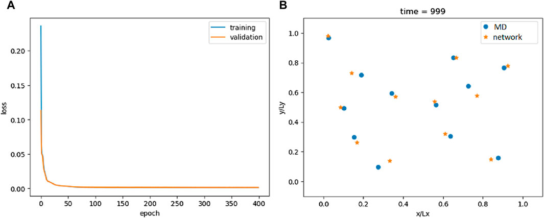
Figure 1. Loss of the FNN model (A) and comparison between the actual and predicted particle positions at the end of the simulation (B).

The first test is the permutability test. In our dataset, particles are given an arbitrary index. However, the dynamics should not be influenced by the index used to order the input data. If we shuffle the indices, the trajectory should remain the same. In the permutability test, we again trained the network, augmenting the training data by randomly shuffling particle indices during training. When particle indices are permuted during training, the model struggles to achieve a low loss, suggesting that the FNN model has not learned the underlying physics but is merely replicating a specific trajectory. The error is approximately 50 times larger than in the non-permuted scenario. Detailed calculations and further information can be found in the notebooks provided in Supplementary Material (refer to the “Code Availability” section for access).

This observation aligns with the physical principles at play. The model is only aware of particle positions, not their velocities. In the non-permuted dataset, it can learn a sequence that corresponds to the evolution of the particles. However, when the particle order is shuffled, this learned sequence becomes disrupted, and without an understanding of the physics, the model cannot infer the correct velocities. Essentially, given the same particle positions at time t−1, the FNN always predicts the same positions at time t. However, identical particle positions can potentially correspond to different velocities. Since the model lacks information about these velocities, it cannot differentiate between these scenarios. In theory, adding velocity data as an input could enhance the model’s performance. However, this would essentially transform the ANN into a complex version of a basic time integrator. While it might improve accuracy, it would not represent a step forward, as the model would be merely replicating a process that can be achieved through simpler computational methods. Based on these considerations, we can establish a permutability criterion that ML models must satisfy.

Criterion 1: the ML model should be invariant under permutation

The second test evaluates the predictive capabilities of the network in two distinct ways. The first is the one-step prediction where the model predicts the state x (t)^ANN based on the real state x (t−1)^MD. This approach tests the model’s ability to accurately predict the immediate next state of the system, i.e.,

$\mathbf{x}(\mathrm{t}{)}^{\text{ANN}}={\mathrm{\varphi }}^{\text{ANN}}\left(\mathbf{x}{\left(\mathrm{t}-1\right)}^{\text{MD}}\right).(1)$

The second is the recursive prediction. In this case, the model’s output for a given timestep is used as the input for the next timestep prediction, i.e.,

$\mathbf{x}(\mathrm{t}{)}^{\text{ANN}}={\mathrm{\varphi }}^{\text{ANN}}\left(\mathbf{x}{\left(\mathrm{t}-1\right)}^{\text{ANN}}\right).(2)$

This iterative process tests the model’s ability to understand and replicate the system’s dynamics over multiple timesteps without relying on real, observed data other than the initial configuration x (0). In the case of the FNN, while the results from the one-step prediction method show a reasonable degree of accuracy, the recursive prediction revealed significant deviations from the observed data over time.

The model’s performance deteriorates as the predictions are based on its own previous outputs rather than real observations (Figure 2). This degradation suggests that while the model is capable of mimicking short-term behavior, it lacks a deeper understanding of the underlying physical principles governing the system. This allows us to formulate a recursability criterion for assessing the network.

Figure 2

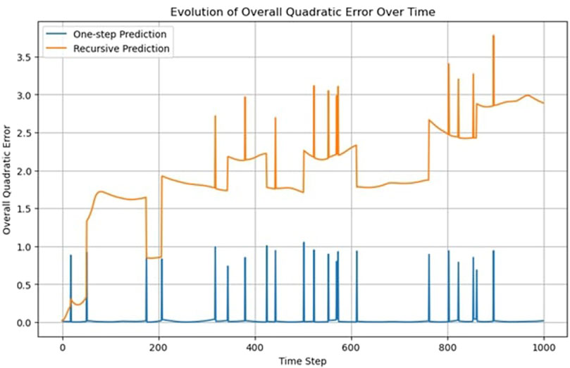
Figure 2. One-step versus recursive predictions of the FNN model.

Criterion 2: trajectories must be predicted recursively, not only from observed data but also from prior predictions

Figure 2 displays sudden jumps in the trajectory’s quadratic error, which can be attributed to the periodic boundary conditions. When a particle crosses the boundary and is repositioned on the opposite side, the predicted position lags in crossing the boundary, resulting in a higher error. A jump of approximately one unit means that one particle is displaced by one boundary length.

Convolutional neural networks

In this section, we explore the process of transforming particle trajectory data into a format suitable for analysis by a CNN. Unlike traditional neural networks, CNNs excel in processing data with a spatial or grid-like structure, such as images. Therefore, the initial task involves converting sequences of particle positions into an image-like representation. The particle trajectory data consist of sequences of x and y coordinates, representing the positions of particles moving over time within the computational domain. To use CNNs, we convert these coordinates into a binary image format representing the presence or absence of particles in different regions of space.

The space is divided into a grid of cells or “pixels,” with each cell representing a specific area of the domain. The size of the grid (e.g., 50 × 50 cells) determines the resolution of our image-like representation. For each timestep, we create an image tensor that will represent the positions of particles as pixels in an image. For each timestep and each particle, we determine the cell in the grid it occupies based on its position. The corresponding cell/pixel in the image tensor is then set to one, indicating the presence of a particle, or zero, indicating the absence of particles. Given that particles do not overlap, dividing the domain into sufficiently small cells ensures that each cell contains at most one particle.

This approach only allows us to establish that a particle is within a cell but not its exact location within that cell. Therefore, the size of these cells is directly proportional to the precision of our spatial data; smaller cells lead to a more accurate representation of particle positions. However, smaller cells result in a larger overall image size, which in turn demands more computational resources and potentially more complex CNN architectures.

The network processes image-like configurations at timestep t−1 as the input and generates the particle configuration image for the subsequent timestep t as the output. A single convolutional layer is employed, demonstrating sufficient accuracy for this task. This layer features an 11 × 11 kernel size, mirroring the cut-off distance used in MD simulation. The model utilizes “circular” mode padding, effectively replicating the periodic boundary conditions characteristic of the MD simulations. The chosen activation function is the sigmoid function as the output is binary, identifying the presence or absence of particles in each image cell.

For optimization, the Adam algorithm is selected with a learning rate of 0.005. The binary cross-entropy (BCE) loss function is used, aligning with the model’s binary classification task. The training and validation losses are shown in Figure 3.

Figure 3

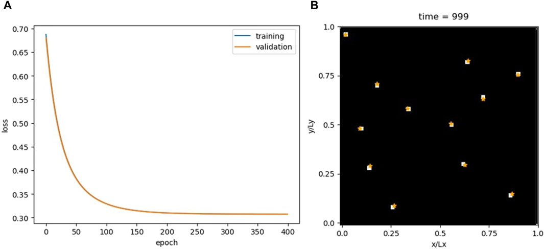
Figure 3. Loss for the CNN model (A) and comparison between the actual and predicted particle positions at the end of the simulation (B). The white squares are the real particle positions converted into pixels of a binary image-like data structure, and the orange stars are the predicted positions.

The CNN demonstrates high accuracy. Supplementary Video S2 compares the MD trajectories with those calculated by the CNN. Furthermore, given the methodology employed in transforming particle positions into images, the sequential order of the particles becomes irrelevant in the image representation. Consequently, by its very design, the model inherently adheres to the permutability criterion.

Despite this, the CNN falls short in fulfilling the recursability criterion. Not only do the predicted trajectories rapidly diverge from actual data but there is also an issue of particle disappearance in the output images. This phenomenon was not observed with the FNN, where each output entry corresponded to a particle’s coordinates. While the FNN’s predictions might place a particle inaccurately, it always represented a particle. In contrast, a CNN’s erroneous output can lead to incorrect images, potentially altering the number of active pixels and, thus, the particle count. This suggests a conservation criterion for assessing a network’s capability in capturing physical dynamics.

Criterion 3: the number of atoms should be strictly preserved

While the conservation criterion can also be applied to other physical properties such as energy or momentum, it is important to note that unlike these properties, which are calculated from the trajectory and, therefore, depend on the accuracy of the model, the preservation of the number of particles is an absolute requirement irrespective of the simulation’s accuracy.

Recurrent neural network

RNNs are a type of artificial neural network designed for processing sequences of data. Unlike FNNs, RNNs have a hidden state that captures information from previous timesteps, making them particularly well suited for tasks involving sequential data such as the time series analysis. In the FNN, we use x (t−1) to predict x (t). Here, we use a sequence-to-sequence RNN that takes three timesteps of the simulation x (t−3), x (t−2), and x (t−1) to predict x (t). The input to the RNN layer corresponds to the system’s degrees of freedom, which is 2N = 24. Its output size, representing the hidden layer of the RNN, was deliberately set to match this value of 24. The RNN is followed by a single linear layer responsible for computing x (t). The loss function and optimization parameters are the same as those used in the FNN.

Supported by an RNN layer, a single linear layer can achieve what required 10 layers in the FNN (Figure 4); Supplementary Video S3 compares MD trajectories with those calculated by the RNN. However, the overall accuracy is lower than that of the FNN (compare the one-step prediction, blue lines, in Figures 2 and 5). Alternative configurations incorporating more previous timesteps as input to the RNN, larger hidden layers, or additional FNN layers yield only marginal improvements.

Figure 4

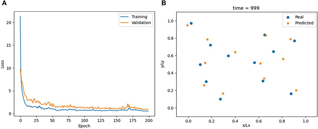
Figure 4. Loss for the RNN model (A) and comparison between actual and predicted particle positions at the end of the simulation (B).

Figure 5

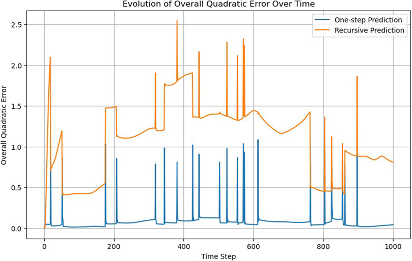
Figure 5. One-step versus recursive predictions of the RNN model.

The RNN, utilizing information from previous timesteps, can learn particle velocities, a capability absent in the FNN and CNN. While this presents an advantage, it becomes problematic when particles cross a boundary and are “teleported” to the opposite side of the computational box due to periodic boundary conditions. This leads to an apparent velocity jump, which is inconsistent with the velocity the RNN has learned from the previous data. This can also be seen in Supplementary Video S3, where the RNN struggles to adapt when the particles cross boundaries. This observation suggests a boundary condition criterion.

Criterion 4: the model should also capture changes occurring at the boundaries

In this study, we exclusively consider “vanilla” RNNs. Gated recurrent unit (GRU) and long short-term memory (LSTM) have the potential to enhance results. However, this is not relevant here since our primary goal is to understand the fundamental characteristics of recurrent networks in their application to MD data rather than maximizing performance. It is this broader perspective that enables us to establish a comprehensive set of criteria for evaluating ML models in the context of particle-based simulations.

Something similar occurs when we look at the recursability criterion (Figure 5). While the RNN does not pass the criterion, the recursive trajectory does not steadily diverge, as occurs in the case of the FNN (Figure 2).

Time convolution

Unlike traditional CNNs, which are predominantly used for spatial data processing, TCs extend this concept to temporal sequences, enabling the analysis of changes in particle positions over time.

Convolutional filters are applied across the sequence x (t−3), x (t−2), and x (t−1), mixing information across these timesteps to predict the state x (t); longer input sequences did not result in substantial improvement. Each particle’s degree of freedom is treated as a separate channel in the input tensor. The kernel size is 3, which is equal to the number of timesteps considered for predicting the next position; no padding is applied.

Overall, the TC model has a good performance, as shown in Figure 6; Supplementary Video S4. It achieves accuracy comparable to the FNN while utilizing a simpler architecture, which consists of only a single TC layer followed by one linear layer. The FNN model required 10 layers to achieve similar results. The TC model is conceptually simpler than the RNN, yet it offers comparable, if not better, outcomes (Figure 7).

Figure 6

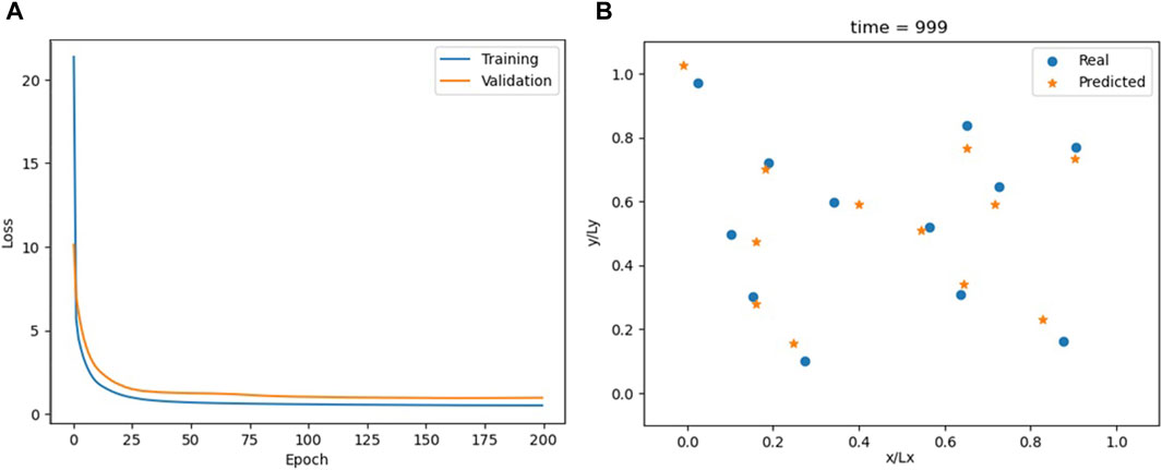
Figure 6. Loss for the TC model (A) and comparison between actual and predicted particle positions at the end of the simulation (B).

Figure 7

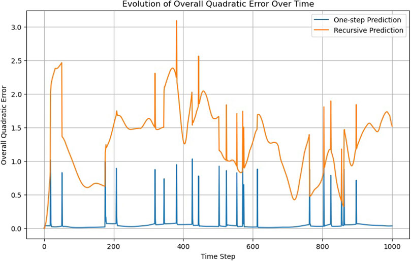
Figure 7. One-step versus recursive predictions of the TC model.

Based on this comparison, we can introduce a simplicity criterion inspired by Ockham’s razor.

Criterion 5: all other things being equal, simpler models should be preferred to more complex ones

Simpler models are beneficial not only in terms of reducing the computational load and memory requirements but also in producing models that are easier to interpret. Based on this criterion, the TC model should be preferred to both the FNN and the RNN models.

Self-attention

Self-attention has recently gained popularity due to its fundamental role in transformers (Vaswani et al., 2017) since it offers a more nuanced approach to sequence data analysis. Unlike traditional convolutional or RRNs, SA allows the model to focus on the most relevant parts of the input sequence regardless of their position within the sequence. Here, the SA model is designed with simplicity in mind, mirroring the input–output structure of the TC model. The sequence of particle positions x (t−3), x (t−2), and x (t−1) goes into an attention layer configured to process the input sequence with a single head and an embedding dimension equal to the number of features (2N = 24). Following the attention layer, the model utilizes a linear layer to refine the context vectors into predictions for the next timestep t.

The performance of the SA model aligns with that of the TC model (Figures 8, 9; Supplementary Figure S10; Supplementary Video S5).

Figure 8

Figure 8. Loss for the SA model (A) and comparison between actual and predicted particle positions at the end of the simulation (B).

Figure 9

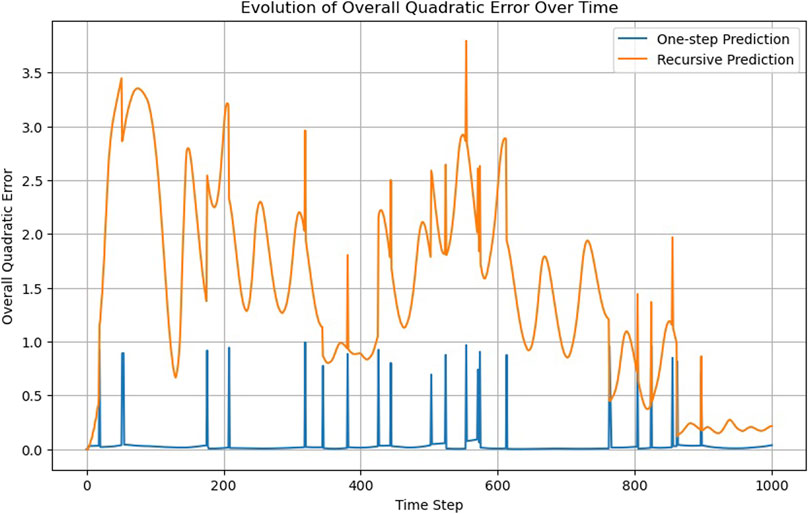
Figure 9. One-step versus recursive predictions of the SA model.

The SA mechanism gives the model the capability to dynamically prioritize the most informative features within the input sequence. This functionality is beneficial in domains such as natural language processing (NLP), where elements spaced far apart within a text may, nonetheless, share profound connections. In these contexts, the correlation function among sequence elements is complex and must be inferred from the data. However, the temporal correlation in MD simulations is more predictable. Due to the chaotic nature of these systems, beyond a certain threshold known as the Lyapunov time, the system forgets its prior states, rendering the two configurations uncorrelated. Time convolutions naturally deal with this aspect of physical systems, while self-attention is made to identify more unpredictable correlation patterns, which do not usually occur in MD systems. Therefore, apart from the simplicity criterion, TC seems to be a better choice over SA because it results in a model that works more like the physics of the system. This leads us to suggest a new naturality criterion.

Criterion 6: models that naturally match our understanding of the system should be preferred

This criterion explains why using a kernel size that matches the MD simulation’s cut-off distance and “circular” mode padding to mimic periodic boundary conditions was especially effective in the CNN model.

Graph neural networks

GNNs are a class of neural networks optimized for processing data within graph structures. In the context of MD or similar particle methods, particles can be seen as nodes in a graph, and the interaction forces between neighboring particles can be seen as edges. Thus, GNNs can appear as a natural choice for such applications, particularly because they inherently meet the permutability criterion due to their design.

However, GNNs demand more input data than other networks; they require not only the input features but also details about the graph’s structure, which is typically provided through matrices such as the adjacency matrix or the edge index matrix (employed here). This requirement poses no issue as long as the graph’s structure remains static. In MD simulations, though, particles and their interacting neighbors change positions during the simulation, leading to non-static edges in the resultant graph.

This leads to two significant challenges: First, the edge index matrix must be recalculated and updated at every timestep to reflect the changing graph structure. Second, the accuracy of the recurrent predictions can be significantly compromised as inaccuracies in particle positions can also lead to errors in the edge index matrix and vice versa. These compounded errors interact and magnify one another, potentially leading the model to increasingly diverge from the actual behavior over time. While GNNs have been applied to model particle trajectories, these applications often necessitate auxiliary routines for updating the neighbor list and, occasionally, additional mechanisms for adjusting positions according to the motion equations (Pfaff et al., 2020). Given the goal of this article to assess GNNs comparably with other models discussed, we restrict the “extra support” for GNNs to merely updating the adjacency matrix at each timestep.

We focus here on one of the simplest GNN architectures, the graph convolutional network (GCN), that aggregates information from neighboring nodes, thereby updating each node’s representation.

The model has five GCN layers, each with 48 hidden neurons, which achieves the best results among the models evaluated. A limitation with GNNs is the potential for excessive layers to induce an unwanted smoothing effect on the nodes, making the addition of more layers not always beneficial. The model’s overall accuracy is noticeably lower compared to the previous section (see Figure 10, Supplementary Video S6), with recursive predictions diverging after a few timesteps (Figure 11).

Figure 10

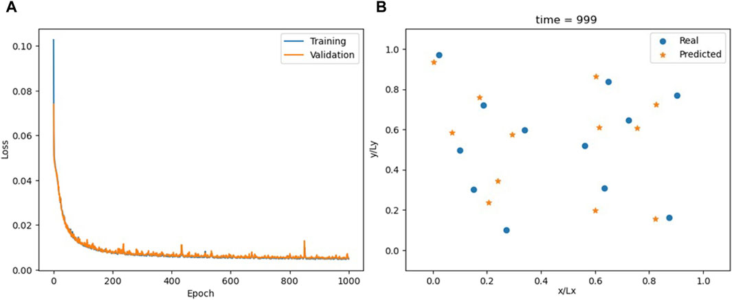
Figure 10. Loss for the GNN model (A) and comparison between actual and predicted particle positions at the end of the simulation (B).

Figure 11

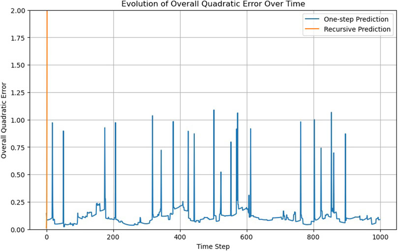
Figure 11. One-step versus recursive predictions of the GNN model.

While GNNs ensure permutability, their simplest and most direct application proves less accurate in this case. Furthermore, the computation of the adjacency matrix for GNNs operates at an O(N²) complexity, contrasting with the O(N^1.5) complexity for calculating the neighbor lists in MD simulations. This discrepancy leads to a scalability criterion.

Criterion 7: the ML model should ideally scale in complexity comparably to the physical model it simulates

Although with only N = 12 particles, scalability is not an immediate concern here. The less efficient scaling of GNNs could become problematic in larger systems.

Physics-informed machine learning

The goal of PIML is to integrate physical laws and principles directly into the structure and training of machine learning models, ensuring that the models not only learn from data but also adhere to the known laws of physics (Cuomo et al., 2022). A standard PIML approach integrates the system’s differential equations into the loss function to enforce adherence to physical laws by penalizing deviations from both observed data and equation-based predictions (Lagaris et al., 1998).

In this study, this would entail incorporating the equations of motion or conservation laws into the loss function. For example, given the simulation’s constant temperature condition, we could adjust the loss function to ensure the particles’ kinetic energy remains constant. However, implementing these solutions necessitates knowledge of time derivatives, such as velocities. Since our prior tests were conducted using only particle positions as input, for consistency, we should maintain the same approach here. In theory, velocities can be inferred from consecutive timesteps. However, when the interval between simulation frames is too large, this method can yield imprecise results. Thus, instead of adjusting the loss function, we chose to embed physics constraints directly into the model’s architecture (Figure 12).

Figure 12

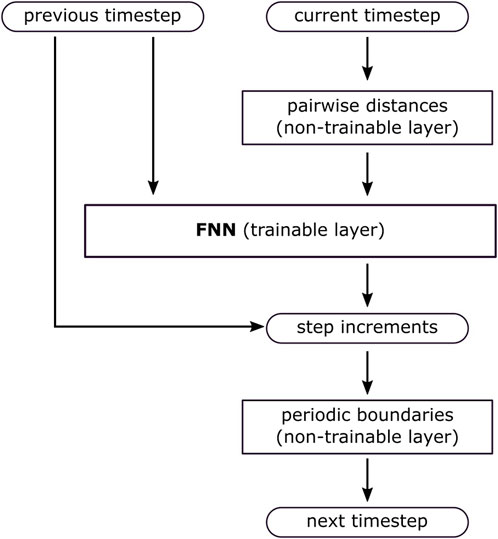
Figure 12. The model’s design embeds information of the system’s physics directly into its architecture.

The model inputs include both the previous and current timesteps. The current timestep is processed by a layer that calculates all pairwise distances among atoms, aligning with the physics of MD simulations where potentials depend on the atoms’ relative distances. This preprocessing layer, which requires no training, also accounts for periodic boundary conditions. Incorporating periodic boundary conditions directly into the PIML model is justified because they are easily observable from the simulation. The previous timestep is the other input, enabling the model to capture the temporal dynamics of the sequence. These inputs are fed into an FNN with five hidden layers, each consisting of 576 neurons. Instead of directly outputting the resulting positions, the network predicts step increments. The next timestep is computed by adding these increments to the current timestep. This solution avoids the abrupt trajectory jumps seen in the previous models and also allows the implementation of periodic boundary conditions in the output.

This method diverges from the conventional PIML, which integrates physics directly into the loss function. The goal here is to construct a model that inherently meets specific constraints (such as periodic boundary conditions) or processes the data to mirror the real system’s behavior (for example, pairwise interactions). This strategy resembles the “minimalistic” method (Alexiadis, 2023; Amato et al., 2024). However, the minimalistic method employs the network only for designated aspects of physics, such as modeling the pair potential from data. Instead of incorporating all computations within the network, it utilizes external solvers for tasks such as calculating the Verlet list or enforcing periodic boundary conditions. These external solvers provide support to the network without being an integral part of it. As a result, the network remains simpler and smaller, focusing only on specific physics components, while external solvers handle the remaining calculations. Therefore, the approach employed here also diverges from the minimalistic method since; rather than delegating physics constraints to external solvers, it integrates them directly into the network as additional non-trainable layers. Consequently, the method cannot be classified as “minimalistic” because the network is neither simplified nor minimized.

Training hyperparameters are the same as in the previous sections; the results are shown in Figure 13; Supplementary Video S7. At first glance, the model appears to overfit. However, the final difference between the training and validation losses is similar to that occurring in Figures 4, 6, 8. It is only the scale of the figure that is different. Moreover, since the model generates incremental outputs, a particle may stay on the incorrect side of the periodic boundary for multiple timesteps. This can lead to substantial numerical errors in relation to the actual position, even though the predicted and real positions are nearly identical when considering periodic wrapping. Further evidence against overfitting is provided in Figure 14; Supplementary Video S8, showing the model’s recursive behavior. During recursive predictions, the model relies solely on the first two timesteps of the real sequence, generating all subsequent steps anew without using data from either the training or validation datasets. The recursive trajectories closely resemble the actual ones, making this the only model investigated that satisfies, at least to a certain extent, the recursability criterion (the permutability criterion, however, is not met).

Figure 13

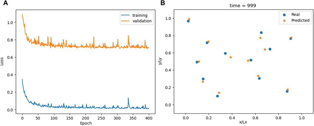
Figure 13. Loss for the PIML model (A) and comparison between actual and predicted particle positions at the end of the simulation (B).

Figure 14

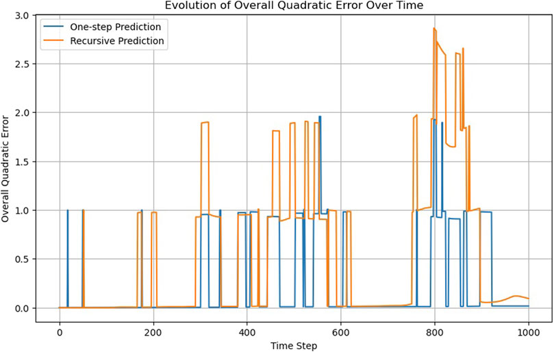
Figure 14. One-step versus recursive predictions of the PIML model.

We can make the recursability criterion more stringent. A “real understanding” of the physics should enable not just the prediction of current trajectories but also the extension of these trajectories to longer simulation times not originally computed by the MD simulation. This observation leads to an extrapolation criterion.

Criterion 8: the model should correctly extend the simulation to longer computational times

To test this criterion, we retrained the PIML model only with the first half of the MD simulation (500 timesteps), and we extended the prediction (both one-step on recursive) to the next 500 timesteps, which the model has never seen (Figure 15).

Figure 15

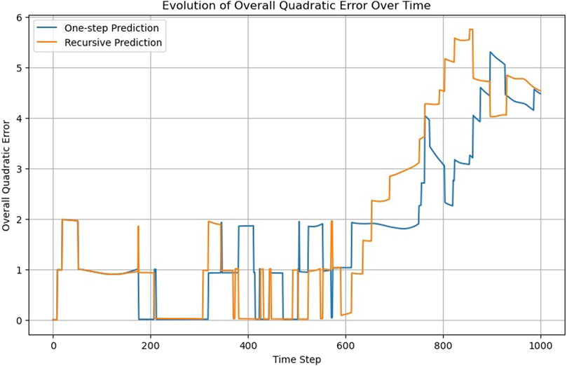
Figure 15. One-step versus recursive predictions of the PIML model trained with only the first half of the MD simulation.

As expected, the model performed well in the first half of the simulation. However, in the next 100 timesteps, the accuracy gradually deteriorated. Therefore, we can assess the extrapolation ability of the model to be around 100 timesteps.

Neural ordinary differential equations

ODENets are a class of deep learning models that integrate neural networks with ordinary differential equations (ODEs). Unlike conventional network architectures that process inputs through discrete layers, ODENets model the transformation of data as a continuous, dynamic process governed by ODEs. This approach allows for a natural handling of temporal data such as those generated from MD simulations. ODENets model the evolution of a system using a set of ODEs.

$\frac{d\mathbf{x}}{dt}=f\left(\mathbf{x},t;\theta \right),(3)$

where x denotes the state of the system, t is the time, and θ is a set of unknown parameters governing the system’s dynamics. The function f captures the system’s rate of change and is approximated by an FNN consisting of five layers, each with 24 neurons. This network, parameterized by θ, is trained to learn the transitions from x (t−1) to x (t) through Eq. 3. However, unlike traditional models where the ML model directly finds x (t) from x (t-1), here, the neural network specifically approximates the function f in this equation.

The ODENet is extremely accurate because Eq. 3 reflects the actual structure of the MD simulation (Figure 16; Supplementary Video S9). However, it does not perform well on the recursability criterion (Figure 17) for t > 600.

Figure 16

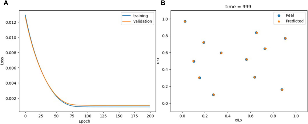
Figure 16. Loss for the ODENet model (A) and comparison between the actual and predicted particle positions at the end of the simulation (B).

Figure 17

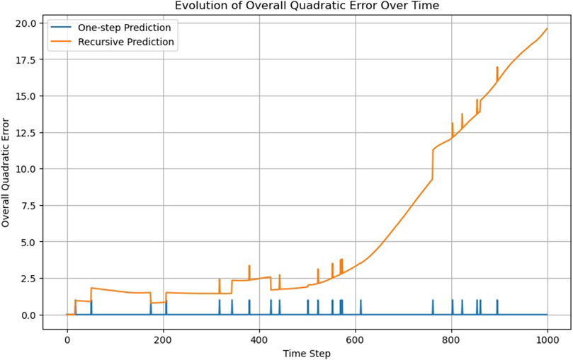
Figure 17. One-step versus recursive predictions of the ODENet model.

Moreover, the ODENet model is continuous in time. While the other models in this study are limited to predicting x (t) at predetermined time intervals, the ODENet’s use of a continuous ODE in Eq. 3 means its outputs are not confined to specific intervals, offering greater flexibility in timestep selection. This flexibility is particularly beneficial, as it enables us to adjust the “granularity” of the simulation, allowing for coarse-graining by using larger timesteps than those in the original time series or for fine-graining to capture more detailed dynamics.

In the one-step prediction, the ODENet model integrates the ODE outlined in Eq. 3 from one sequence element at time t to the next at time t+1. Unlike other networks, ODENets are not confined to single timesteps; the ODE can be integrated over t+α, where α = 2 corresponds to a two-step prediction, α = 3 to a three-step prediction, and so forth. Notably, α is not limited to integer values. Figure 18 compares the error across different α values, demonstrating that even with a timestep 10 times larger than the original, the error remains modest, at approximately 2%. This observation introduces the granularity criterion.

Figure 18

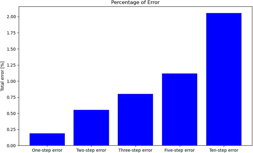
Figure 18. Comparative analysis of prediction errors across multiple timesteps for the ODENet model.

Criterion 9: the ML model should enable granularity adjustments, enabling both coarse-graining and fine-graining of the predictions

The primary challenge with the ODENet model lies in the potentially higher computational cost compared to the original physics-based model. While both approaches involve solving the series of ODEs in Eq. 3, the f function of the ODENet has more parameters and is numerically more complex than its physics-based counterpart. This observation leads to the formulation of an economy criterion.

Criterion 10: ideally, the ML model should not surpass the physics-based model in computational demands

We must also consider that our analysis involves only a limited number of particles. In particle simulations with millions of particles, if the network’s goal is to replicate trajectories, its size will grow with the increase in the degrees of freedom. A straightforward approach, similar to the one applied in this study, could result in extremely large and computationally demanding networks.

Additional criteria

Based on our previous work on integrating physics-based solvers with ML models (Alexiadis, 2023; Lagaris et al., 1998; Alexiadis, 2019b; Alexiadis and Ghiassi, 2024), we can propose two additional evaluation criteria to account for features that could not be tested in the neural networks examined in this article.

A good indication of a model’s grasp of the systems’ physics would be its ability to predict MD trajectories under the conditions, such as pressure or temperature, that are beyond the range of the initial training dataset. This introduces an extensibility criterion.

Criterion 11: the model should reproduce conditions besides the training dataset

In principle, expecting a model to perform accurately beyond its training data seems too optimistic. However, while this criterion may not generally be met, there are scenarios where, to a certain degree, this has been achieved (Alexiadis, 2023; Amato et al., 2024).

Finally, we did not compare the training times of the models in this study, primarily because such comparisons are challenging to conduct on equal footing. To make a meaningful comparison, it would be necessary to optimize all models, a step we did not undertake as it falls outside the scope of this paper. Despite this, we acknowledge the importance of efficiency during training, leading us to propose a somewhat obvious training-time criterion.

Criterion 11: the model’s training time should not be excessively long, especially when compared to the duration required for the physical simulations it aims to replicate.

Generally, a network requires only one training phase, allowing for the allocation of additional time to this process if it results in an accurate ML model. However, this criterion highlights that there are practical limits to the amount of time that can be reasonably allocated to training.

Conclusion

This article establishes a set of criteria for assessing ANNs trained to replicate trajectories derived from MD simulations. We individually examined the several fundamental network architectures in machine learning: FNN, CNN, RNN, TC, SA, GNN, ODENet, and an example of PIML. As expected, none of these networks meet all the criteria. The FNN falls short of the permutability criterion, the CNN does not satisfy the conservation criterion, and the RNN does not meet the boundary condition criterion. TC and SA have a similar performance, but TC is preferable according to the naturality criterion. The GNN meets the permutability criterion but fails the scalability one. All networks, except, perhaps, the PIML (which fails the permutability and extrapolation criteria), do not meet the recursability criterion. Moreover, while the ODENet is extremely accurate, it also requires more computational time for solving the ODEs, which goes against the economy criterion. These conclusions focus on atomic trajectories, not macroscopic properties that can be statistically derived from trajectories, such as temperature, pressure, or transport properties such as thermal diffusivity or viscosity (Papastamatiou et al., 2022; Stavrogiannis et al., 2023; Sahputra et al., 2020).

While it is possible that combining these networks as layers within more complex networks may enhance the performance in specific cases, our primary objective in this paper is to independently assess the advantages and disadvantages of each network type. The rationale behind this focused examination is to lay a groundwork upon which future research can build more effective and nuanced combinations of neural network layers. By identifying the specific strengths and weaknesses of individual architectures, researchers and practitioners can make more informed decisions when designing advanced models that integrate multiple layers or architectures.

Data availability statement

The datasets presented in this study can be found in online repositories. The names of the repository/repositories and accession number(s) can be found at: github.com/alexiada/criterias-for-data-based-MD.

Author contributions

AA: writing–original draft and writing–review and editing.

Funding

The authors declares that no financial support was received for the research, authorship, and/or publication of this article.

Conflict of interest

The author declares that the research was conducted in the absence of any commercial or financial relationships that could be construed as a potential conflict of interest.

Publisher’s note

All claims expressed in this article are solely those of the authors and do not necessarily represent those of their affiliated organizations, or those of the publisher, the editors, and the reviewers. Any product that may be evaluated in this article, or claim that may be made by its manufacturer, is not guaranteed or endorsed by the publisher.

Supplementary material

The Supplementary Material for this article can be found online at: https://www.frontiersin.org/articles/10.3389/fnano.2024.1373316/full#supplementary-material

References

Alexiadis, A. (2019a). Deep multiphysics and particle–neuron duality: a computational framework coupling (discrete) multiphysics and deep learning. Appl. Sci. Basel, Switz. 9 (24), 5369. doi:10.3390/app9245369

CrossRef Full Text | Google Scholar

Alexiadis, A. (2019b). Deep multiphysics: coupling discrete multiphysics with machine learning to attain self-learning in-silico models replicating human physiology. Artif. Intell. Med. 98, 27–34. doi:10.1016/j.artmed.2019.06.005

PubMed Abstract | CrossRef Full Text | Google Scholar

Alexiadis, A. (2023). A minimalistic approach to physics-informed machine learning using neighbour lists as physics-optimized convolutions for inverse problems involving particle systems. J. Comput. Phys. 473 (111750), 111750. doi:10.1016/j.jcp.2022.111750

CrossRef Full Text | Google Scholar

Alexiadis, A., and Ghiassi, B. (2024). From text to tech: shaping the future of physics-based simulations with AI-driven generative models. Results Eng. 21, 101721. doi:10.1016/j.rineng.2023.101721

CrossRef Full Text | Google Scholar

Alexiadis, A., Simmons, M. J. H., Stamatopoulos, K., Batchelor, H. K., and Moulitsas, I. (2020). The duality between particle methods and artificial neural networks. Sci. Rep. 10 (1), 16247–7. doi:10.1038/s41598-020-73329-0

PubMed Abstract | CrossRef Full Text | Google Scholar

Alhajeri, M. S., Abdullah, F., Wu, Z., and Christofides, P. D. (2022). Physics-informed machine learning modeling for predictive control using noisy data. Chem. Eng. Res. Des. Trans. Institution Chem. Eng. 186, 34–49. doi:10.1016/j.cherd.2022.07.035

CrossRef Full Text | Google Scholar

Amato, E., Zago, V., and Del Negro, C. (2024). A physically consistent AI-based SPH emulator for computational fluid dynamics. Nonlinear Eng. 13 (1). doi:10.1515/nleng-2022-0359

CrossRef Full Text | Google Scholar

Cuomo, S., Di Cola, V. S., Giampaolo, F., Rozza, G., Raissi, M., and Piccialli, F. (2022). Scientific machine learning through physics–informed neural networks: where we are and what’s next. J. Sci. Comput. 92 (3), 88. doi:10.1007/s10915-022-01939-z

CrossRef Full Text | Google Scholar

Jenis, J., Ondriga, J., Hrcek, S., Brumercik, F., Cuchor, M., and Sadovsky, E. (2023). Engineering applications of artificial intelligence in mechanical design and optimization. Machines 11 (6), 577. doi:10.3390/machines11060577

CrossRef Full Text | Google Scholar

Karniadakis, G. E., Kevrekidis, I. G., Lu, L., Perdikaris, P., Wang, S., and Yang, L. (2021). Physics-informed machine learning. Nat. Rev. Phys. 3 (6), 422–440. doi:10.1038/s42254-021-00314-5

CrossRef Full Text | Google Scholar

Lagaris, I. E., Likas, A., and Fotiadis, D. I. (1998). Artificial neural networks for solving ordinary and partial differential equations. IEEE Trans. neural Netw. 9 (5), 987–1000. doi:10.1109/72.712178

PubMed Abstract | CrossRef Full Text | Google Scholar

Papastamatiou, K., Sofos, F., and Karakasidis, T. E. (2022). Machine learning symbolic equations for diffusion with physics-based descriptions. AIP Adv. 12 (2), 025004. doi:10.1063/5.0082147

CrossRef Full Text | Google Scholar

Pfaff, T., et al. (2020). Learning mesh-based simulation with graph networks, international conference on learning representations. Available at: http://arxiv.org/abs/2010.03409 (Accessed February 3, 2024).

Google Scholar

Reynolds, C. W. (1987). “Flocks, herds and schools: a distributed behavioral model,” in Proceedings of the 14th annual conference on Computer graphics and interactive techniques (New York, NY, USA: ACM).

CrossRef Full Text | Google Scholar

Sahputra, I. H., Alexiadis, A., and Adams, M. J. (2020). A coarse grained model for viscoelastic solids in Discrete Multiphysics simulations. ChemEngineering 4 (2), 30. doi:10.3390/chemengineering4020030

CrossRef Full Text | Google Scholar

Stavrogiannis, C., Sofos, F., Sagri, M., Vavougios, D., and Karakasidis, T. E. (2023). Twofold machine-learning and molecular dynamics: a computational framework. Computers 13 (1), 2. doi:10.3390/computers13010002

CrossRef Full Text | Google Scholar

Thai, H.-T. (2022). Machine learning for structural engineering: a state-of-the-art review. Structures 38, 448–491. doi:10.1016/j.istruc.2022.02.003

CrossRef Full Text | Google Scholar

Vaswani, A., et al. (2017). Attention is all you need. Available at: http://arxiv.org/abs/1706.03762 (Accessed February 13, 2024).

Google Scholar