
94% of researchers rate our articles as excellent or good
Learn more about the work of our research integrity team to safeguard the quality of each article we publish.
Find out more
ORIGINAL RESEARCH article
Front. Mol. Biosci. , 01 June 2023
Sec. Protein Biochemistry for Basic and Applied Sciences
Volume 10 - 2023 | https://doi.org/10.3389/fmolb.2023.1122269
This article is part of the Research Topic Computational and Experimental Protein Variant Interpretation in the Era of Precision Medicine View all 10 articles
 Germano Nobili1,2
 Simone Botticelli1,2
 Giovanni La Penna3,2*
 Silvia Morante1,2,3Giancarlo Rossi1,2,4Gaetano Salina2
We present an improved application of a recently proposed computational method designed to evaluate the change of free energy as a function of the average value of a suitably chosen collective variable in proteins. The method is based on a full atomistic description of the protein and its environment. The goal is to understand how the protein melting temperature changes upon single-point mutations, because the sign of the temperature variation will allow us to discriminate stabilizing vs. destabilizing mutations in protein sequences. In this refined application the method is based on altruistic well-tempered metadynamics, a variant of multiple-walkers metadynamics. The resulting metastatistics is then modulated by the maximal constrained entropy principle. The latter turns out to be especially helpful in free-energy calculations as it is able to alleviate the severe limitations of metadynamics in properly sampling folded and unfolded configurations. In this work we apply the computational strategy outlined above in the case of the bovine pancreatic trypsin inhibitor, a well-studied small protein, which is a reference for computer simulations since decades. We compute the variation of the melting temperature characterizing the folding-unfolding process between the wild-type protein and two of its single-point mutations that are seen to have opposite effect on the free energy changes. The same approach is used for free energy difference calculations between a truncated form of frataxin and a set of five of its variants. Simulation data are compared to in vitro experiments. In all cases the sign of the change of melting temperature is reproduced, under the further approximation of using an empirical effective mean-field to average out protein-solvent interactions.
Many proteins are characterized by a given three-dimensional structure when they are observed in a water soluble monomeric state Branden and Tooze (1999). In order to understand the way the sequence determines the structure, the effect of single point mutations has been studied since a long time Cunningham and Wells (1989). A simple way to address the sequence-structure interplay is to measure some structural parameter as a function of temperature. Circular dichroism (CD) and many other techniques are often used and in many cases the change of this structural parameter with temperature can be taken as an indicator of the melting of the protein structure Cantor and Schimmel (1980). The change of melting temperature triggered by different single point mutations is therefore a widely used measure of the change of protein stability upon a localized change of the protein sequence and large archives of such data have been collected Guerois et al. (2002); Alexov and Sternberg (2013); Forbes et al. (2016). When this information is available, it must be interpreted in terms of the reshaping of atomic interactions.
The change of protein stability upon sequence mutations has implications in many pathologies. One example is Friedreich’s ataxia, an autosomal-recessive genetic condition that causes ataxia, sensory loss and cardiomyopathy worsening over time Pandolfo (2009); Klockgether (2011); Clark et al. (2018). The cause of the disease is in mutations of the gene encoding for the frataxin (FXN) protein. Depending on the specific kind of mutation, a patient may end up with an insufficient level of frataxin, a nonfunctional frataxin or frataxin, that is, not correctly localized in the mitochondria Delatycki et al. (2000); Galea et al. (2016). Frataxin variants have also a role in cancer, as expected because of the involvement of FXN and mitochondria in the control of oxidative metabolism Schulz et al. (2006). Indeed, missense variants are found in multiple human cancer tissues Petrosino et al. (2019, 2021). The example of FXN shows that even single point mutations can have significant impact in protein stability, trafficking, plasticity, interactions with local environment and mutual interactions with other macromolecules.
Many models have been proposed to relate measured changes in protein stability with the chemical nature of the protein sequence. High through-put approaches based on atomic models have been recently developed Steinbrecher et al. (2017). Many of these approaches are summarized in this Special Issue.
The method we would like to propose here aims at predicting the change of thermal stability of a protein in a monomeric water-soluble state, when its sequence is changed by a single aminoacid. The method is based on a suitable modelling of interatomic forces, i.e., it is atomistic, and includes an explicit model of the water solution. The method was initially applied to FXN Botticelli et al. (2022) and it is here refined and discussed in more detail, to achieve better computational performance and higher accuracy in prediction. In particular, we use here the well-tempered metadynamics, one of the best performing method to enhance sampling of phase space in atomistic models. A small reference protein of 58 residues is first used to assess the methods and to understand limitations and advantages.
Many initial configurations of the protein of interest are generated, assuming the protein structure representing the native state of the wild-type sequence, but with initial conditions diversified as much as possible. This is achieved by changing the protein environment, that is, in this case the water solution of NaCl. A multiple walkers metadynamics simulation is carried out Raiteri et al. (2006); Hošek et al. (2016); Hošek et al. (2017), building an external biasing potential as a function of a suitably chosen collective variable. In the range of values spanned by the collective variable folded and unfolded protein structures are sampled.
The external potential is built so as to initially unfold the protein structure. All along the metadynamics simulation time, the external biasing potential is systematically constructed and updated to uniformly sample folded and unfolded configurations. This goal is best achieved by combining multiple walkers histories into a unique trajectory Hošek et al. (2017).
The standard analysis of multiple walkers metadynamics can be performed, but limitations in predicting experimental behaviours arise because of the huge number of configurations required to achieve a good convergence and stability. We therefore decided to exploit the features of the maximal constrained entropy approach which allows to properly re-modulate the collected set of sampled configurations by imposing suitable conformational constraints. In this way we can reliably monitor the change in free energy as a function of average values of the chosen collective variables. The quantity of interest to be calculated is therefore:
where the subscript denotes a sequence (the pedix 0 indicates a reference sequence, usually the wild-type), and the s state variable indicates the degree of structural order, where s0 indicates the folded native state and s indicates the unfolded state.
The approach is first applied to the study of a paradigmatic protein displaying a well defined three-dimensional structure, namely, to the bovine pancreatic trypsine inhibitor (BPTI), where the effect of a set of mutations on melting temperature has been carefully investigated Yu et al. (1995). BPTI has always been a milestone for folding studies, being one of the smallest proteins (58 aminoacids) characterized by a well defined structure. Then, the same procedure is applied to frataxin, in a truncated form of 121 aminoacids, and 5 of its variants Petrosino et al. (2019).
The computational methods used in this work are similar to those used in Ref. (Botticelli et al., 2022). In the following we emphasize the differences that characterize this work.
Let ξ(q) be a collective variable (CV) function of atomic positions, q. When ξ is an observable quantity, the values, s, allowed for ξ can be used to label system macrostates. The set of coordinates q labels the system microstates, each set of q yielding one of the possible values of s. If ergodicity holds, infinitely long simulations of a trajectory q(t) in a given statistical ensemble would correctly sample the statistical weight of ξ. However, because of the huge number of ways in which certain values of s of ξ are encountered, compared to others, actual numerical simulations in practice only sample the maximally degenerate values of ξ. This is precisely the case where ξ is the CV associated to folding/unfolding events.
Standard statistical ensembles and more recently generalized ensembles try to address this problem by biasing the trajectory to spend more time where ξ has a low degeneracy and less time where ξ has a large degeneracy.
The sampling of configurations obtained with the biased inverse probability of ξ is called metastatistics. We will denote by
Many methods have been proposed to sample configurations with the inverse of the estimated probability of ξ Mitsutake et al. (2001). In this work and in the previous application of the method Botticelli et al. (2022), we used the altruistic metadynamics proposed in Refs. Hošek et al. (2016); Hošek et al. (2017). The desired metastatistics is obtained from a swarm of trajectories provided by metadynamics after building a suitable external bias, which is then kept fixed when collecting configurations in the final step of the NpT simulation (see Section 2.6). We performed simulations in the statistical ensemble associated to constant temperature T and pressure p (NpT ensemble) because macromolecules forced by an external bias undergo large and fast conformational changes. When these conditions occur, solute macromolecules exert strong perturbations over the explicit solvent and ions representing their environment. To cope with steep changes of kinetic energy of water molecules and possible temporary voids around the macromolecule, the NpT ensemble is recommended.
In the framework of metadynamics, the estimated probability of the CV is expressed by means of a sum of Gaussian functions, VG [ξ(q)], related to the inverse metastatistics probability by the formula
with β = 1/(kBT) where T is the temperature used in the simulation, kB the Boltzmann constant, and C a normalization constant, that is, of no relevance in the computation of thermal averages. Different methods have been proposed to build an external bias VG [ξ(q)] such that the probability distribution of ξ is flat and transitions between folded and unfolded states of a biomolecule endowed with many degrees of freedom, are equally well sampled.
In metadynamics the external potential VG (ξ, t) acting on the system at time t is defined as:
where t′ < t, s(t) = ξ(q(t)) is the value taken by the CV at time t, w is the Gaussian height, δ is the Gaussian width τG is the time interval after which a new Gaussians is added.
After a sufficiently long time VG(s, t) provides an estimate of the underlying free energy F according to the formula
where C(t) depends on time but not on the collective variables s, VG is the external biasing potential acting on the system at time t.
Equation above states that an equilibrium quantity, like free energy, can be estimated by a non-equilibrium dynamics in which the bias potential is changed in time, as new Gaussians are successively added. In metadynamics, when all the wells in CV distribution are filled with Gaussians, the dynamics in the CV space becomes diffusive.
Well tempered metadynamics is an improved approach designed to obtain a reliable estimator of the free energy Barducci et al. (2008). The weight of each Gaussian function added to the bias VG depends on the history of VG (VG(t′)). Equation 3 changes into:
where kBΔT is approximately the energy change when a new value of ξ is visited. An exact relation between VG(s, t) and F(s) can be obtained if the rate at which the bias potential is modified is suitably decreased as the simulation progresses. With well tempered metadynamics, the biasing potential converges to
The quantity
For a finite T, the probability distribution is proportional to:
which corresponds to effectively increasing the CV sampling temperature. Thus, the effect of well tempered metadynamics is similar to that of other non-equilibrium methods, like steered molecular dynamics, but trajectories are obtained with a quasi-equilibrium procedure Bussi et al. (2018).
In well tempered metadynamics, as the simulation proceeds the width of the added Gaussian remains constant but its height decreases (see Eq. 5). The bias, which increases monotonically, eventually changes very slowly with time. At the beginning the space of CV is flooded by Gaussians of height w. With the progress of flooding, heights of newly added Gaussians decrease. This behaviour is very important in highly complex biological systems, where the bias potential should never reach any excessively large value.
In contrast with the “non tempered” metadynamics, in the well tempered metadynamics a flat CV distibution is not expected to be achieved when convergence is obtained. A simple interpretation of the fact that the distribution of the CV at long times is not flat is the following. Since the prefactor for the accumulated Gaussians depends on the value of s, Gaussians of different heights are placed in different regions of the CV space. In order to reach a stationary distribution, it is thus necessary that the system spends more time in regions where small Gaussians are added and less time in regions where large Gaussians are added. This idea can be pushed further and used to convert metadynamics in an algorithm, not designed to flatten completely (as in non-tempered metadynamics) or partially (as in well tempered metadynamics) the histogram of the CVs but rather to enforce a predefined distribution Bussi et al. (2018).
In this work we used a biasing factor of 20 (see Eq. 6), corresponding to ΔT = 5700 K, in agreement with the biasing factor used in literature for similar molecular systems Hošek et al. (2017). The energy value RΔT is of the order of a typical energy barrier of a single hydrogen bond.
The maximal constrained entropy method (MEC method, hereafter) allows, starting from
where
In an infinitely long (ergodic) simulation, it is unnecessary to explicitly evaluate the weights
In case of the “non tempered” metadynamics, the maximal constrained entropy was employed as a viable solution to compute thermal averages as a function of the average values taken by the chosen CV, in situations where metastatistics is not fully ergodic and the CV distribution does not come out flat. As mentioned, in the case of well tempered metadynamics the CV distribution is not expected to be flat, but the maximal constrained entropy method is a powerful method to “correct” the free energy by adding ex post further information about the system injecting extra information. In our case we use the maximal constrained entropy to introduce in the computation of the free energy the change of number of hydrogen bonds in α-helices in folding↔unfolding processes. In general the maximal constrained entropy method can be used either to improve the estimate of the free energy for a non-converging system (e.g., in a metadynamics simulation the CV distribution is not flat) or to compute the free energy by reintroducing ex post degrees of freedom related to the CV (like the α-helices’ hydrogen bonds in the case of frataxin, see Section 3). This second use of the maximal constrained entropy method is really powerful because allows to have a reliable estimate of the free energy while keeping efficient the simulations by limiting the degrees of freedom of the system.
The main goal of this work is to compare the change of free energy as a function of the number of hydrogen bonds (s) computed using well tempered metadynamics and maximal constrained entropy, with the results obtained in protein thermal denaturation experiments Yu et al. (1995); Petrosino et al. (2019). Both BPTI and FXN are folded in a structure where one or two α-helices lay over a small β-sheet. The experimental measurement of the free energy difference between folded and unfolded states was obtained by measuring the molar ellipticity at 222 nm, a wavelength where the contribution of α-helix to CD spectra is dominant. Besides acting on the α-helices arrangement, the protein ternary structure can also be perturbed by destroying the intra-molecular hydrogen bonds that stabilize the β-sheet. For a small protein like BPTI (58 residues), we decided to include in the CV all the hydrogen bonds that are formed in the native folded state Parkin et al. (1996). For FXN (121 residues) we took instead as a CV the number of hydrogen bonds occurring in the β-sheet formed by 4 anti-parallel β-strands, which are observed both in 1EKG and 5KZ5 structures Botticelli et al. (2022). This choice in the case of FXN was made to reduce the number of degrees of freedom of the system thus substantially decreasing the time required to sample its phase space. The use of such CV as a way to monitor the structural transitions in the protein was inspired by several previous applications of metadynamics Barducci et al. (2006).
For both proteins and variants, the biasing potential, VG, was obtained at the end of a systematic construction (well tempered metadynamics) in which VG is progressively built by summing over Gaussian functions of the CV. Gaussian functions (possibly scaled by the biasing factor in the case of the well tempered metadynamics) are deposited every 20 ps along the molecular dynamics (MD) simulation time.
The accumulated final biasing potential, VG(ξ), smoothly interpolated by a polynomial of fourth order, was used for the direct computation of the change in the free energy for folded to unfolded states and vice versa. The free energy change defined in well tempered metadynamics is given by Eq. 6:
with s0 a reference state corresponding to a given value of the CV and VG the external biasing potential determined at the end of construction. Equation 9 holds also in the NpT statistical ensemble, when the construction of the bias VG is performed in such statistical ensemble. In this case, the Helmoltz free energy F(s) is replaced by the Gibbs free energy G(s). We call the latter function G free energy, hereafter, for simplicity. The G free energy extracted from well tempered metadynamics simulations (Eq. 9), was then compared with the G free energy obtained with the maximal constrained entropy method.
The accumulated statistics used in the successive maximal constrained entropy application have been obtained by collecting the system configurations along a trajectory where the biasing potential was kept fixed (i.e., not anymore updated). Within the maximal constrained entropy method, the definition of the G free energy (see La Penna et al., 2004) is given by the formula
in which G(s) is written as the combined sum of the enthalpy in the NpT ensemble, and the (informational) entropy measured by the maximal cross-entropy. In Eq. 10 H = U + pV is the enthalpy of the simulated system, λ the parameter associated with the constraint,
The maximal cross-entropy in Eq. 10 is described in the following. Given an estimate,
is solved by determining the maximum of the cross-entropy functional Attard (2000); La Penna (2003); La Penna et al. (2004).
under the constraint (Eq. 11). The well-known solution of this variational problem is given by the formulae:
with the parameter λ the solution of the (highly non-linear) equation:
The quantity exp (−λξγ)/Zλ is called the modulation factor of the metastatistics. Owing to Eq. 15, λ is a function of s. Inserting the solution for Pγ into Eq. 12 one gets for the cross entropy at its maximum:
The average of H (or simply of U in NVT simulations) is obtained using equations like
with B either H or U and
The details to compute the free energy within the maximal constrained entropy method, the direct calculation of ⟨H⟩λ in Eq. 10 as well as the free energy error estimate is the same we used in our previous work where the “non tempered” version of the metadynamics Botticelli et al. (2022) was employed. In this work we concentrate on collecting more accurate averge quantities (well-tempered metadynamics and longer simulations) and on applying the proposed method also to a simpler protein (BPTI). We must note that the direct calculation of ⟨H⟩λ in Eq. 10 includes the effects of the fluctuations of U and V due to the movement of all explicit water molecules and ions included in the atomistic model of the protein environment. The fluctuations of H are huge, while the change of the average of H with s is small. This is a serious issue when using the total enthalpy like in Eq. 10. As it is customary done in these cases, we use an approximate evaluation of ⟨H⟩λ, where H is replaced by the effective mean-field free energy
A widely used strategy for the evaluation of the effective mean-field energy of the solute protein is the so-called molecular mechanics/Poisson-Boltzmann solvent accessible approximation (MM/PBSA) Simonson et al. (2002). In this approach the mean-field energy for solute-solvent interactions is described as the sum of polar (electrostatic) and non-polar (surface) contributions. For each protein configuration Q one writes
where Uintra is the intra-molecular part of the potential energy in the protein force-field, given by
The various contributions are the stretching (Ustr), bending (Ubend), and torsional (Utors) terms in the potential. Uvdw and Uel are the Lennard–Jones and Coulomb interactions, respectively, computed by summing over all the pairs of atoms of the protein.
The last two terms in Eq. 18 represent solute-solvent contributions to free energy at fixed Q. Mean field energy is the energy as a function of Q once the variables associated to solvent positions and velocities are averaged for the given value of solute positions Q. The averaging is performed at the given thermodynamic state variables p and T used in the simulation of the whole system. Within this mean-field assumption, the solute and the solvent are made independent. This is a strong approximation, since the chosen collective variable contains the number of hydrogen bonds within protein groups and once a single intramolecular hydrogen bond is broken there is a large chance for the formation of hydrogen bonds with the water molecules in the protein environment where the breaking event occurs. On the other hand, this elementary change of free energy, that does not imply a wide change in protein structure, can be calculated within the MM/PBSA approximation as the sum of Gsolv,np and Gsolv,pol. Therefore, under this approximation, the change of free energy G(s) depends on the number of protein configurations for which a unitary change of s is allowed independently of the configuration of the protein environment. The calculation of Gsolv,np and Gsolv,pol is described in the following.
The term Gsolv,np is the contribution to the solute-solvent free energy due to the formation of a cavity of zero charge density with the shape of the solute protein and the creation of the solute-solvent interface. Introducing a charge density in the space occupied by the solute leads to the Gsolv,pol contribution. The charge density is given in terms of the point charges qi of the atom i sitting at the point
The term Gsolv,np is calculated as an empirical linear combination of the solvent accessible surface area (SASA) for each group in the solute molecule Ooi et al. (1987) according to the formula
where the coefficients σi are positive or negative for hydrophobic or hydrophilic groups, respectively (see below for details). Finally the electrostatic contribution to the solute-solvent free energy, Gsolv,pol, is given by the electrostatic energy required to charge the low-dielectric solute molecule of generic shape into a high-dielectric medium like a salt-water solution. The magnitude of this contribution is obtained by a numerical finite difference solution of the Poisson–Boltzmann equation Rocchia et al. (2002).
We summarize the complicated computational protocol of our theoretical analysis as follows. One starts by performing MD simulations at T = 300 K in the presence of the biasing potential VG(ξ) built according to the well tempered metadynamics strategy. The resulting statistics is what we call metastatistics. Using the set of collected configurations, we determine the λ parameter that maximizes the cross-entropy Sc in the maximal constrained entropy method, under the constraint ⟨ξ⟩ = s. In the case of BPTI, ξ is the number of hydrogen bonds holding together the protein α-helices and β-sheet secondary motifs. In this case, the ξ of metadynamics and that of maximal constrained entropy coincide. In the case of BPTI, differently from FXN (see below), the ξ collective variable takes into account the whole of the secondary structure as it is observed in the crystal folded structure. Therefore, s takes integer values in the range between 0 and 16. In the case of FXN, the variable ξ used in metadynamics is the number of hydrogen bonds holding together the protein β-sheet (made of 4 anti-parallel β strands). The values of s are in the range between 0 and 15. But in the maximal constrained entropy approach we extended ξ adding to it the number of hydrogen bonds in the two α-helices. For each value of s, we get a value of λ that yields the modulating weight
with q the system configuration at time t, indexing the microstate γ, along the collected metadynamics trajectory. For details see Ref. (Botticelli et al., 2022).
Apart from the fact that differently than what was done in Ref. (Botticelli et al., 2022), in this work the metastatistics is obtained as altruistic multiple-walkers well-tempered metadynamics, most of the technical details of the simulation procedure we followed to compute the expectation values of the physical quantities of interest described in Section 2 are identical to those reported for FXN in Ref. (Botticelli et al., 2022). Below we only outline the few differences.
Table 1 provides the list of hydrogen bonds used to define the CV for the BPTI. All the hydrogen bonds contribute to the BPTI CV and are used both in well tempered metadynamics and maximal constrained entropy. For FXN only the number of hydrogen bonds in the β-sheet, β1−4, is used to generate the statistics of metadynamics. However, the total number of hydrogen bonds listed in Table 1 of Ref. (Botticelli et al., 2022), including the two α-helices added to the definition of CV in the successive maximal constrained entropy step. We call this an extension of the CV ξ used in metadynamics and we indicate it with ξ′. The corresponding constrained average is indicated with s′.
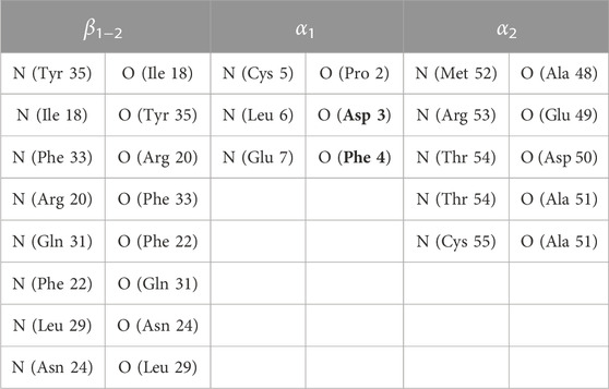
TABLE 1. Pairs of atoms used in Eqs 16–18 of Ref. (Botticelli et al., 2022) and related label in parameter S. As for FXN, see Table 1 of the same publication. Residues are those of BPTI WT sequence. Mutated residues are boldface.
Table 2 reports the number of atoms of the two systems (BPTI and FXN) we have studied. In the case of BPTI, the structure of the unique folded structure available [1BPI PDB entry Parkin et al. (1996)] has been used. As for FXN, the initial configurations of the various walkers are obtained using the available crystallographic information about the native FXN protein sequence. We used two structures: the X-ray structure of the mature human frataxin [PDB 1EKG, segment 88-210 Dhe-Paganon et al. (2000)]; the structure of FXN in the mitochondrial iron-sulfur cluster assembly machine as it was determined by electron microscopy (PDB 5KZ5, chain A, segment 42-210 Gakh et al. (2016)).
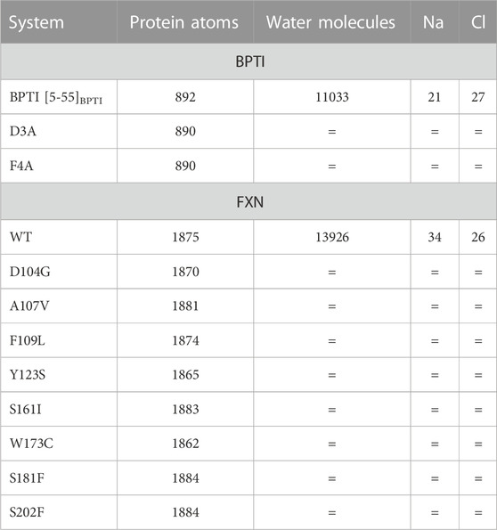
TABLE 2. Short description of the atomistic models used in metadynamics simulations. The composition of each system changes only in the protein sequence for each protein (BPTI and FXN, respectively). The number of water molecules and counterions (NaCl) is the same for all the 90 walkers representing each system, and the same (= symbol) for different variants of the same protein.
The values of α and w of Eq. 3 in Ref. (Hošek et al., 2017) and used in the successive stages of the simulation are reported in Table 3. As for the construction of the biasing potential, we remark that its construction in the present work lasted 22 ns, while in our previous application it lasted 16 ns. The exchange of the bias among walkers takes place every 2 ns. At the end of stage 15 (see Table 3), i.e., after simulating each walker for a total of 30 ns using an altruistically updated bias, the external bias that will be used in stage 16 and in the following steps is not updated any more. From stage 16 to the end the final metastatistics is collected, storing configurations along the simulated trajectory every ps. The time duration of this last simulation step was 10 and 30 ns for BPTI and FXN, respectively.

TABLE 3. Short description of the simulation stages used to build the external bias VG(ξ) and to acquire the metastatistics at constant external bias. Where α and w are not indicated, the external bias is not updated. The initial bias is zero. Therefore, stages 1–3 (6 ns) are equilibration stages. The bias construction is the same for all variants of BPTI and FXN. As for the constant bias simulation stage 16–20 (10 ns) were collected for BPTI, while 16-30 (30 ns) were collected for FXN. Values of α and w are used when applying the altruistic combination of single-walker updating (2 ns) of VG using Eq. 3 of Ref. (Hošek et al., 2017). The resulting global altruistic bias is used in the following 2-ns stage (next line). The bias after stage 15 is approximately the same for all walkers and, therefore, is made identical for all walkers by averaging over the 90 walkers.
48 single point mutations have been studied in the case of BPTI in the literature Yu et al. (1995) via alanine-scanning. This set of mutations includes all residues, with the exception of 6 Ala and 4 Cys, mutated to Ala. The reference sequence used to study the change in melting temperature is the native sequence where Cys 14, 30, 38, and 51 are mutated in Ala. This reference variant is indicated as [5-55]BPTI, to underline the presence of the residual 5–55 disulfide bridge. The sequence is used because the native sequence has 3 disulfide bridges in the folded structure and it does not unfold at T < 100°C. The removal of 2 disulfide bridges allows the melting at T < 50°C, while the protein keeps the same folded structure as the native (WT) sequence, as summarized in Ref. (Yu et al., 1995). Therefore, we could use the structure determined for the WT sequence as the initial representation of the folded state (1BPI Parkin et al. (1996) in PDB).
According to our conventions, a positive ΔΔG means a larger reversible work required to unfold the given variant with respect to the reference sequence. All the variants analyzed in experiments have been already studied as part of large data-sets in previous works dedicated to predictions of free energy change Guerois et al. (2002); Steinbrecher et al. (2017). In our work we are interested in predicting the sign of the free energy change, which is also the sign of the change of the melting temperature Tm, ΔTm. As paradigmatic cases we focused, among the 48 variants, on the two displaying the largest measurable change in the absolute value of ΔTm. The mutations with the most positive and negative value of ΔTm [see Table 1 in Ref. (Yu et al., 1995)] are D3A and F4A, respectively.
Three representative structures of the [5-55]BPTI reference sequence of BPTI. are displayed in Figure 1 to show how the folded (left panel) and unfolded (right panel) states look like in terms of atomic configurations. Native BPTI is folded into a ternary structure with two short α-helices and a small β-sheet. The construction of the external bias, VG(ξ), perturbs the ternary structure by breaking the intramolecular hydrogen bonds.
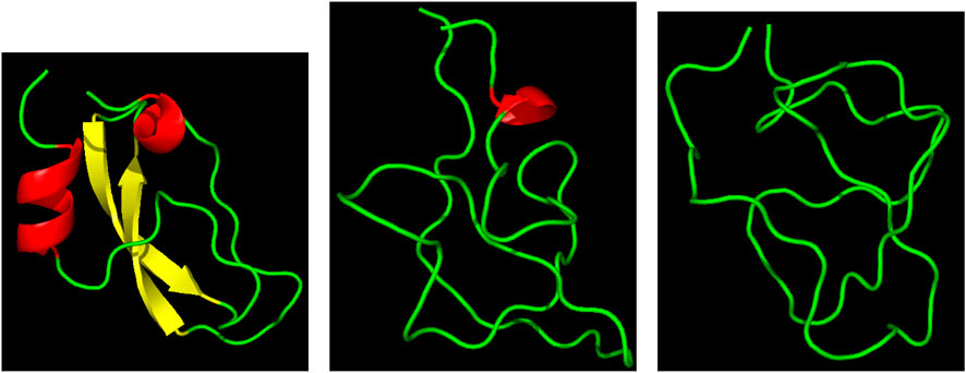
FIGURE 1. Three representative structures of [5-55]BPTI reference sequence of BPTI. Left—ξ = 13 (folded state); middle—ξ = 4 (unfolded state); right—ξ = 4 (unfolded state). α-helices are in red; β-sheet is in yellow; the displayed ribbon interpolates the backbone atoms. The Pymol program is used for the molecular drawing Schrödinger (2015).
This is why we decided to take as a collective variable ξ the sum of the number of hydrogen bonds between the two α-helices (α) and the β-sheet (β). The number of hydrogen bonds of α-helices and β-sheets in the initially folded structure (PDB 1BPI) is 8 for both secondary structures. Therefore, the values of ξ span the range between 0 and 16. Figure 1 shows in the right panel that the unfolded state is represented by a molten globule. This occurs because of the short-range nature of the collective variable we have chosen. In the specific case of BPTI the presence of the residual disulfide bridge 5-55 that seals the N-terminus with the C-terminus also pushes the protein towards this atomic arrangement.
The evolution in time of the collective variable ξ is notoriously slow, even by using well tempered metadynamics. Therefore the convergence of the external bias VG(ξ) is expected to occur after very long simulation times. This issue is illustrated in Figure 2, where the time evolution of ξ of 4 walkers among 90 is displayed. We remind that every 2 ns the bias VG obtained by the whole set of 90 walkers is exchanged among all of the walkers during bias construction in the altruistic approach [Eq. 3 in Hošek et al. (2017)]. Furthermore, before the bias construction the 90 walkers have been separately equilibrated for 8 ns. The figure is divided in two parts. The time evolution during the 22 ns of bias construction is displayed on the lefthand side. The time evolution at constant bias, which constitutes the metastatistics used to compute the biased equilibrium averages, during the last 10 ns is displayed in the righthand side. The figure clearly shows that the unfolding of the protein often occurs during bias construction, since ξ decreases from the value characterizing the folded state to values of 3–4 in 3 cases over the 4 displayed. In certain cases (red curve) the expected behaviour of a random walk of ξ in the 3–14 range is observed.
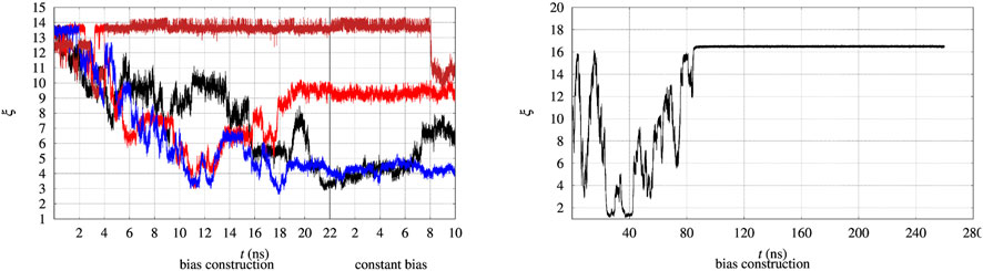
FIGURE 2. Time evolution of the collective variable ξ during the bias construction (left part) and at constant bias (right part), with the vertical line dividing the bias construction from the bias application. Left—The evolution is displayed in different colors for 4 representative walkers among 90 and for BPTI in the [5-55]BPTI sequence. Right—The same evolution is displayed for a single walker in well-tempered metadynamics of FXN in the WT sequence.
In principle metadynamics is capable of letting the system, starting from the known folded configuration, to unfold and refold. In practice this rarely occurs in affordable computational time, unless the system is sufficiently small. To illustrate the time-scale required for collecting such trajectory, the behaviour of ξ for the longer FXN chain is displayed in Figure 2 (right panel) for a single walker. In this trajectory a single-walker well-tempered metadynamics is performed for 260 ns. While the first 100 ns of the trajectory displays an ideal behaviour for metadynamics [see for instance Figure 2 in Ref. (Barducci et al., 2006)], when the bias is no more effectively updated by new Gaussian functions the system becomes frozen in a fixed configuration. This effect is expected in well-tempered metadynamics, since the height of the Gaussian functions that are added to the bias is progressively decreased by construction.
Anyway, the dynamics of ξ shows that in order to observe a proper random walk of ξ for all walkers, simulation time should have been at least 10–100 times larger. The dynamics of ξ becomes even slower when the bias is kept constant compared to bias construction (righthand side of both panels in Figure 2). This behaviour is due to the effect of noise during bias construction, occurring when new Gaussian contributions are added to VG every 10 ps. The dynamical nature of VG during its construction acts as a stochastic perturbation. This effect is not present when VG is kept constant and when VG does not change because added Gaussian heights are small.
Because of the slow dynamics of ξ, the metastatistics represents a static disorder triggered by the bias construction process.
In Figure 3 we display the behaviour of VG(ξ) during the bias construction for the BPTI reference sequence. The red arrow indicates the direction in which the iteration index of the altruistic method, occurring every 2 ns of metadynamics simulation, increases. In the process of iteration the number of Gaussian contributions to VG keeps increasing in the region of low ξ values, while at high ξ it does not change anymore after the first 4 iterations. A full convergence of VG is not achieved, but we notice that the change of VG is very slow after about 10 iterations. This happens because when the protein is unfolded, many atomic configurations consistent with a low number of hydrogen bonds are possible. Then, Gaussian contributions to VG are all added in the region of low ξ values, while no further contributions are added to the region of high ξ values.
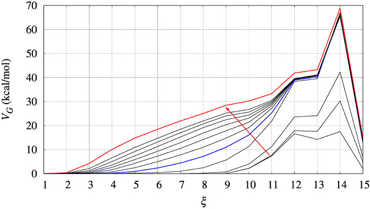
FIGURE 3. The evolution of the bias (VG) acting on walker 1 during bias construction for BPTI, [5-55]BPTI sequence. Different curves are obtained combining the bias of all walkers using Eq. 3 of Ref. (Hošek et al., 2017). The red arrow indicates the increasing iteration. The red curve is that used in the final collection, while the blue curve was used to estimate the effect of a non-converged bias on the values of free energy obtained by the post-processing MEC method.
Since the bias converges very slowly, it is worth checking the effect of choosing different bias in the calculation of interest for us, that is, ΔΔG as a function of the chosen collective variable for a protein variant with respet to the wild-type sequence. In Figure 3 we choose the red curve, as what we assumed as converged bias, and the blue curve, the function built after 5 iterations in the altruistic scheme (stage 9 in Table 3). The difference between results obtained with these two different choices of final bias will be described later for BPTI. We remark that the configurations used in the comparison are the results of two different 10-ns trajectories for all of the 90 walkers: one performed with the “converged” bias (stage 15 in Table 3) while the second performed with the bias of stage 9.
Times of the order of 100 ns are required to build a useful bias for each walker even for a protein of 58 residues like BPTI. This issue is illustrated by the behaviour of a single walker of the larger FXN protein (see Figure 2, right panel, discussed above). In practice such long simulation times can not be used to compare a native sequence with the usually rather large number of its variants. The method described in this article allows extracting differences in stability under point variations with computational wall-times of the order of 1 month in a high-performance computing infrastructure.
In Figure 4, left panel, we display the free energy change ΔΔG computed using Eq. 9, implicitly assuming that VG has properly converged after 22 ns of multiple-walkers bias construction. In Figure 5, we also display the free energy change using the polynomial of order 4 interpolating the grid representation of the bias VG (see Section 2.4). We remind that the polynomial interpolation is performed on each approximately converged VG(ξ) profile obtained by metadynamics. Therefore, the effect of interpolation on the free energy change ΔΔG as a function of sequence change can be slightly different when the difference between interpolated curves is extracted. In Figure 6 we display the comparison between the grid representation of ΔG = −VG + C and its interpolation in all of the three sequences investigated for BPTI. We notice that for the three variants the free energy increases by decreasing the value of the collective variable, consistently with a greater thermal stability of the protein configurations in the folded state. But, because of the smoothing of VG exerted by the interpolation, part of the changes are lost. However, even the tiny difference between the curves ΔG = G(ξ)—G(ξ0) is still a representation of the change in stability upon protein unfolding once the sequence is changed. In the BPTI case, we find that, consistently with experiments (see Table 4), the D3A mutation induces an increase in the stability of the protein (left panel, red curve). The opposite is true for the F4A mutation.
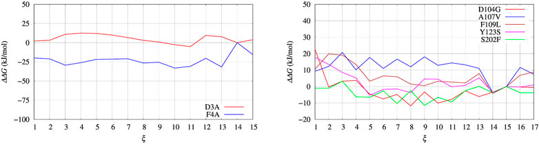
FIGURE 4. Free energy change (ΔΔG) calculated with Eq. 9 and VG built with well tempered metadynamics. Left panel: BPTI; Right panel: FXN.
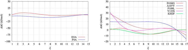
FIGURE 5. Same as for Figure 4 using the polynomial of order 4 interpolating the grid representation of the bias VG used in Figure 4. Left panel: BPTI; Right panel: FXN.
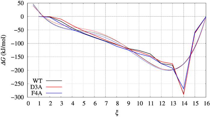
FIGURE 6. Same as for Figures 4, 5 (left panels), but comparing ΔG(ξ) for the case of BPTI variants. Color scheme is black, red, and blue for WT, D3A, and F4A variants, respectively. Thick line is the grid representation of VG; thin line is the 4-th order polynomial interpolation of each grid (same color) in the range between 0.5 and 15.5. Out of this range the interpolation is linear, with continuous derivative at the extreme points.
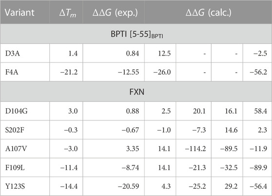
TABLE 4. Experimental (ΔTm, °C), experimental ΔΔG Petrosino et al. (2019), and computed values of ΔΔG (kJ/mol) for the selected BPTI and FXN variants. Column 4: the values obtained with metadynamics. Columns 5-7: the maximal constrained entropy method is used with the effective energy for solute-solvent interactions (Eqs 18, 19). Column 5—Data published in previous article Botticelli et al. (2022); column 6—Simulation used in previous article, using the extended ξ′ variable in the maximal constrained entropy method; column 7—Well tempered metadynamics, using the extended ξ′ variable in the maximal constrained entropy method. Rows are reported in descending order of ΔTm for each protein. While for BPTI the collective variable ξ = α + β is used both in metadynamics and maximal constrained entropy methods, for FXN ξ = β is used in metadynamics and the extended variable ξ′ = ξ + α = β + α is used in the maximal constrained entropy method. β is the number of hydrogen bonds in the β-sheet; α is the number of hydrogen bonds in the α-helices (see Methods for details). BPTI: Unfolded state is s = 4; Folded state is s = 14 (highest peak in the distribution obtained with the meta-statistics, see Figure 7). FXN: Unfolded state is s′ =21 [23 for simulation of Ref. (Botticelli et al., 2022)]; Folded state is s′ =37.
As discussed above, statistics severely limits the convergence of VG(ξ), since the number of Gaussian contributions to VG giving an almost flat ξ distribution is achieved when all unfolded configurations are sampled, a condition, that is, hardly achieved even with μs-long MD simulations. Employing multiple walkers allows one to sample unfolded and folded configurations in non-infinitely long simulation but each of the walkers is not able to walk from a folded configuration towards an unfolded one and viceversa with a frequency allowing a proper sampling.
In the left panel of Figure 7 we display the distribution of the collective variable ξ along with the sampling at constant bias VG(ξ) for all the BPTI variants. The distributions that we obtain are not flat because of the technical limitations of the well tempered metadynamics method (see Section 2.2) and the limited span of sampled CV values as shown in Figure 2 and discussed above. Despite the sampling being likely insufficient to have both a converged bias and a converged distribution of ξ once a constant bias is applied, we can estimate the reversible work necessary to build a given average of ξ, s, from the biased metastatistics at our disposal. This is done using the maximal constrained entropy approach described in Ref. (Botticelli et al., 2022) and references therein.
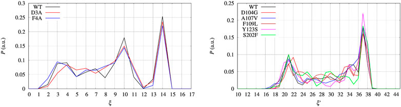
FIGURE 7. Distribution P as a function of the collective variable ξ. Left panel—BPTI, where ξ = β + α, where β and α are the number of hydrogen bonds in, respectively, the β-sheet and α-helices present in the folded structure. Right panel—FXN, where ξ = β was used to build the external bias, but the extended variable ξ′ = β + α is used to represent the distribution. P is normalized as to have ∑iPi = 1, where Pi is each of the displayed values.
The free energy difference between each of the two variants of BPTI D3A and F4A, and the reference sequence [5-55]BPTI is displayed in the left panel of Figure 8 as a function of the average value s of the collective variable ξ (see Section 2). The MEC modulation is employed here and Eq. 1 is used, with X sequences identified by different colors. Since the distribution of ξ in the metastatistics displays a sharp peak in the folded state (ξ = 14) and a broad peak in the unfolded one (at about ξ ∼ 4) we report in Table 4 the free energy change going from the state of average s = 14 (that is, the state s0 in Eq. 1) to the state with average s = 4.
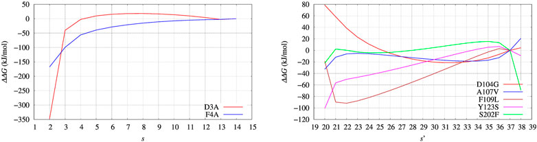
FIGURE 8. Changes of free energy variation (ΔΔG) upon unfolding, that is, the decrease of the average number of hydrogen bonds in α helices and β-sheets, α and β, respectively. The average is s = ⟨(α + β)⟩. As for FXN (right panel) the number of hydrogen bonds is calculated after using metadynamics based on ξ = β and ξ′ = α + β in the maximal constrained entropy method. Color scheme is the same as for Figure 7.
The direct metadynamics calculation and the maximal constrained entropy method give consistent results for the sign of ΔΔG in the case of BPTI. In fact, we find a slightly negative value equal to −2.5 kJ/mol for D3A at s = 4 (see Table 4; Figure 8, left panel). Moreover, in both cases our results are consistent with experiments. It is important to recall that among the 48 single-point mutations of [5-55]BPTI, only 3 produces a stabilization of the protein Yu et al. (1995).
Before entering into structural details providing explanation of ΔΔG values, we assess what we expect to be the major source of error propagation in the MEC method. The most efficient handle to expand the sampling of atomic protein configurations is the external bias VG, as computed by well-tempered altruistic multiple-walkers metadynamics. Therefore, we calculated ΔG(s) profiles for BPTI, which is protein small enough to easily repeat 900 ns of MD simulations, using two different choices of VG(ξ), respectively the red and blue curves in Figure 3. The profiles of ΔG(s) computed with the different choices are displayed in Figure 9, left and right panels, respectively, for red and blue curves of VG(ξ). We notice that there are a few values that are affected by the limited number of points in the statistics: s = 2 (left panel) and s = 4 (right panel). By using the bias obtained by a shorter cumulative history (the blue curve), low values of ξ (contributing to low values of average s) are rarely sampled. Apart from these limitations due to the range of sampled ξ values, the similarity in the behaviour of G(s) is remarkable. In particular, we notice that the sign of ΔΔG (the difference between curves in each of the plots) is robust. This depends on the fact that the contribution to the calculation of ΔGs with the help of Eq. 10 depends on the energy of the populated states (with a certain value of the collective variable ξ) rather then to the number of ways the state is reached by the simulation.
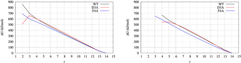
FIGURE 9. BPTI: change of free energy (ΔG) upon unfolding, that is, the decrease of the average number of hydrogen bonds in α helices and β-sheets, α and β, respectively. The average is s = ⟨(α + β)⟩. Left panel is obtained with Eqs 10, 18, using the configurations collected for 10 ns with the final bias obtained (red curve in Figure 3); Right panel is obtained using the configurations collected for 10 ns with an intermediate bias, blue curve in Figure 3. Color scheme is the same as for Figure 7.
Due to the collection of atomic configurations at hand and to the possibility of computing the different terms contributing to ΔΔG, we can interpret the unusual stabilization of the D3A variant observed in experiments. The increase in unfolding free energy upon D3A mutation is partially due to the removal of the salt-bridges formed by Asp 3 that occur in the WT sequence. On the other hand, the F4A mutation reduces the steric hindrance of Phe 4 thus enhancing the chance of salt-bridges formation between the N-terminus and other protein regions. The competition between electrostatic long-range contributions and short-range interactions characterizing the hydrophobic patches can be analyzed studying the changes in the terms contributing to U.
In Table 5 the change in four terms contributing to U (see Eqs 18, 19) are reported, together with the whole change of U (last column). The latter dominates the change of G, since the contribution of the maximized cross-entropy is small compared to ΔU in Eq. 10. The significant changes in each component almost cancel each other in the sum. The smaller change in Uvdw in the F4A case indicates the cancellation of hydrophobic contacts between Phe 4 and the residues in the major hydrophobic core of folded BPTI when Phe 4 is replaced by Ala. The negative change of Usolv,np for all variants indicates the release of hydrophilic sidechains into the solvent upon unfolding. This contribution tends to cancel the release of dispersive solute-solute interactions. However, the two electrostatic contributions (ΔUel and ΔGsolv,pol) span the largest range of values among the variants. Therefore, we argue that changes in the electrostatic networks become critical with respect to an almost uniform background of interactions that change upon the demolition of the hydrophobic core occurring during unfolding.
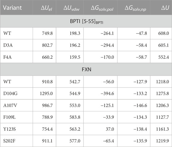
TABLE 5. Energy changes (kJ/mol) starting from folded reference state, ending to unfolded state for native (WT) sequence and studied variants. Folded and unfolded states are defined as in Table 4. The energy components are those indicated in Eqs 18, 19.
Most of the long-range salt-bridges lock the native structure into a less hydrophilic globular form, because the small size of the globule allows efficient electrostatic sealing, not allowed when the size of the globule increases. Breaking of the salt-bridges in the native form allows exposing hydrophylic groups to the solvent while the formation of the salt-bridges hides hydrophobic groups inside the globule core. Once salt-bridges are broken, that is, when the hydrogen bonds keeping the native scaffold are broken, the globular protein is allowed to expose a larger surface to the solvent, including its hydrophobic core.
In conclusion, the D3A stabilization against protein unfolding is due to the stabilization of non-native salt-bridges when the native Asp 3 is removed.
Our analysis has shown that for the small BPTI protein (58 residues) the number of configurations at constant bias we have been able to collect provides consistency between well tempered metadynamics and the maximal constrained entropy method. On the other hand, the improvement of statistics we achieve in this work, compared to our previous investigation of the FXN case, as explained in the next section, is not yet sufficient to get full consistency and robust predictions in the case of bigger proteins.
The effects of single-point mutations on the unfolding process of the truncated form of FXN (residues 90-210) have been discussed in detail in Ref. (Botticelli et al., 2022). Differences of the present work compared to what was done in the previous paper are the following:
1. The well tempered metadynamics method is employed in place of a plain (constant T) metadynamics;
2. The construction of the biasing potential is made with a larger number of iterations and is, therefore, more accurate;
3. The maximal constrained entropy method is applied here using an extended collective variable including the number of hydrogen bonds present in the folded α-helical regions;
4. The trajectory produced at constant bias, which is used in the maximal constrained entropy method, is three times longer than in Ref. (Botticelli et al., 2022).
The change of G computed using the bias VG(ξ) as obtained out of 22 ns of bias construction is displayed in the right panels of Figures 4, 5. Again, the free energy increases upon unfolding (decrease of ξ), in agreement with what happens in similarly folded state as observed in experiments Petrosino et al. (2019) (data not shown here). However, the relative order of unfolding free energy is not well captured. Indeed, most of the variants are found to be more stable than the WT reference sequence. On the other hand, in experiments only the D104G variant among the 8 analyzed shows an increased stability of the folded state with respect to the native sequence and, therefore, a larger unfolding free energy.
An explanation of the difference between the trend showed by experiments and that predicted by direct metadynamics is in the choice of the collective variable we made to study FXN unfolding. The thermal unfolding was measured by CD at 222 nm wave-length: this means that the CD signal was mainly composed by variations in the content of α-helices. The choice of ξ = β in metadynamics was based on the expectation that the demolition of the β-sheet would be sufficient to destabilize all the secondary motifs in the protein, including the two α-helices. This was only partially true. In Figure 10 we show the distribution of α, the number of hydrogen bonds in α-helices, in correspondence low and high values of β, 4 and 15, respectively. The distributions were computed making reference to the 30-ns long simulation at constant bias collected for the whole set of 90 walkers. The curve with β = 4 shows that α-helices are partially broken in those configurations where the β-sheet is broken. This effect is due mainly to the shortening of helix α1 (data not shown here), which is softer than α2 particularly in its N-terminus. Therefore, only an a posteriori analysis of the effect of a chosen collective variable can point to a more valid collective variable to be used in metadynamics.
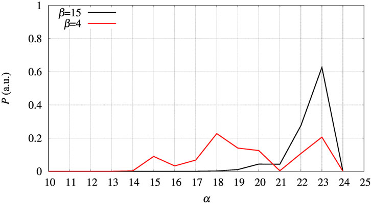
FIGURE 10. The distribution of α obtained in the 30-ns trajectories collected for the whole set of 90 walkers at constant bias Vg(β) for FXN, WT sequence. Black curve—Distribution obtained for configurations with β = 15; red curve—Same distribution with β = 4.
The set of configurations, obtained by including all the 90 walkers simulated at constant bias, is used in the maximal constrained entropy method to overcome the above shortcoming. Results for FXN are displayed in the right panels of Figures 7, 8. In Figure 7 (right panel) we notice that the two peaks at s′ = 21 and 37 are not due just to the choice of initial configurations (i.e. the two PDB structures used to differentiate the walkers, see Section 2). The distance in s′ between the two peaks displayed in Figure 7 (right panel) is larger than the difference in α-helical values between the two PDB structures used to build the set of initial configurations, namely 37-21 compared to 23-19. Consistently with the data displayed in Figure 10, this means that the metastatistics contains configurations with a significant decrease in the number of α-helical hydrogen bonds despite the external bias forcing the unfolding being a function of the number of hydrogen bonds in the β-sheet only.
In the right panel of Figure 8 the profiles of ΔΔG of the 5 different variants studied with maximal constrained entropy method are compared. It is interesting to notice that the relative order of the experimental values of ΔTm (see also Table 4) is better reproduced with the use of the augmented and updated statistics collected in this work.
The different contributions to ΔΔG are reported in Table 5. Again, the tendency of different contributions to compensate each other when summed is apparent. It can be noticed that, similarly to BPTI, the electrostatic contributions display a larger span among variants. In the case of D104G the value of ΔUel is clearly dominant, while the opposite sign contribution of the polar solvation term is unable to compensate the effect of changes in direct electrostatic contacts. Strikingly, despite the longer accumulation of statistics and the more accurate bias construction, the reasons of the D104G stabilization can be explaind in terms of the same effects described in the previous investigation Botticelli et al. (2022). It is the removal of Asp 104 that changes the structure of the α1 helix and the possibility of the charged residues lying in that region to form alternative salt-bridges. When α1 helix is allowed to rotate, like in the unfolded molten globule, these interactions are not possible. However, the effect of the point mutation on the S202F variant is different as the change of dispersive interactions become significant, consistently with the introduction of a hydrophobic sidechain (Phe) in place of the small hydrophilic Ser residue. In this situation, it is possible to infer that the native-like hydrophobic core is stabilized and more work is required to destroy it and the significant change in electrostatic interactions (ΔUel) is seen to positively combine with hydrophobic contributions.
Though the interactions among protein atoms and between the protein and its environment (a NaCl solution) are crudely approximated, the method is able to capture the little changes surviving when the total potential energy is computed.
In this work we refined the combination of several computational methods to predict, on the basis of fully atomistic protein models, the changes of thermal stability of proteins under single-point mutations. The method has been applied to a well-studied small protein, the bovine pancreatic trypsin inhibitor (58 residues), and to a truncated form of frataxin (121 residues). In both cases experiments were compared to computational results. The unusual effect of protein stabilization exerted by some point mutations was the special focus of this study.
We found a good agreement in the sign of representative values of ΔΔG upon unfolding and the sign of the shift in the melting temperature compared to experimental results. The competition between the changes in the demolition of hydrophobic cores and the changes in networks of electrostatic interactions is captured by the method. This effect was not fully analyzed in the interpretation of the unusual D3A stability in BPTI, so far.
Despite its potential, the method is computationally quite demanding, requiring extended statistical methods and, as for the collection of reliable configurations, a detailed model for atomic interactions, including explicit solvent and counterions. As discussed in the case of FXN, the direct calculation of free energy variation from the constructed bias potential is strongly affected by the choice of the collective variable in metadynamics. It was found that the maximal constrained entropy is a possible work-around to the statistical limitations of even challenging and promising methods like those based on multiple-walkers well tempered metadynamics. Numerical limitations still prevent the application to many interesting variants where the native structure becomes unstable: F33A, F22A, Y35A for BPTI; W173C for FXN. The ability of predicting the sign of the free energy change is in any case of extreme importance when the protein can adopt structures alternative to the native one.
The raw data supporting the conclusion of this article will be made available by the authors, without undue reservation.
GN and SB made most of the reported calculations. GL designed the method and the application. GR described the method within statistical physics. SM and GS acquired the funds to perform the work. All authors equally contributed to data interpretation and manuscript writing.
This work was supported by the project PRIN-201744NR8S (MIUR, Italy) and the BIOPHYS initiative (INFN, Italy). Numerical calculations have been made possible owing to the projects IscrB_PolyFrat, IscrC_PolyBPTI, and the CINECA-INFN agreement, all providing us access to computational resources on MARCONI-100 at CINECA.
The authors declare that the research was conducted in the absence of any commercial or financial relationships that could be construed as a potential conflict of interest.
All claims expressed in this article are solely those of the authors and do not necessarily represent those of their affiliated organizations, or those of the publisher, the editors and the reviewers. Any product that may be evaluated in this article, or claim that may be made by its manufacturer, is not guaranteed or endorsed by the publisher.
Alexov, E., and Sternberg, M. (2013). Understanding molecular effects of naturally occurring genetic differences. J. Mol. Biol. 425, 3911–3913. doi:10.1016/j.jmb.2013.08.013
Attard, P. (2000). The explicit density functional and its connection with entropy maximisation. J. Stat. Phys. 100, 445–473. doi:10.1023/A:1018668502023
Barducci, A., Bussi, G., and Parrinello, M. (2008). Well-tempered metadynamics: A smoothly converging and tunable free-energy method. Phys. Rev. Lett. 100, 020603. doi:10.1103/PhysRevLett.100.020603
Barducci, A., Chelli, R., Procacci, P., Schettino, V., Gervasio, F. L., and Parrinello, M. (2006). Metadynamics simulation of prion protein: β-Structure stability and the early stages of misfolding. J. Am. Chem. Soc. 128, 2705–2710. doi:10.1021/ja057076l
Botticelli, S., La Penna, G., Nobili, G., Rossi, G., Stellato, F., and Morante, S. (2022). Modelling protein plasticity: The example of frataxin and its variants. Molecules 27, 1955. doi:10.3390/molecules27061955
Branden, C., and Tooze, J. (1999). Introduction to protein structure. London, UK: Garland Publishing Inc.
Bussi, G., Laio, A., and Tiwary, P. (2018). Metadynamics: A unified framework for accelerating rare events and sampling thermodynamics and kinetics. (Cham Springer Int. Publ., 1–31. doi:10.1007/978-3-319-42913-7_49-1
Cantor, C. R., and Schimmel, P. R. (1980). Biophysical chemistry. San Francisco, USA: W.H. Freeman & Co.
Clark, E., Johnson, J., Dong, Y., Mercado-Ayon, E., Warren, N., Zhai, M., et al. (2018). Role of frataxin protein deficiency and metabolic dysfunction in friedreich ataxia, an autosomal recessive mitochondrial disease. Neuronal Signal 2, NS20180060. doi:10.1042/NS20180060
Cunningham, B. C., and Wells, J. A. (1989). High-resolution epitope mapping of hgh-receptor interactions by alanine-scanning mutagenesis. Science 244, 1081–1085. doi:10.1126/science.2471267
Delatycki, M. B., Williamson, R., and Forrest, S. M. (2000). Friedreich ataxia: An overview. J. Med. Genet. 37, 1–8. doi:10.1136/jmg.37.1.1
Dhe-Paganon, S., Shigeta, R., Chi, Y.-I., Ristow, M., and Shoelson, S. E. (2000). Crystal structure of human frataxin. J. Biol. Chem. 275, 30753–30756. doi:10.1074/jbc.C000407200
Forbes, S. A., Beare, D., Boutselakis, H., Bamford, S., Bindal, N., Tate, J., et al. (2016). Cosmic: Somatic cancer genetics at high-resolution. Nucleic Acids Res. 45, D777–D783. doi:10.1093/nar/gkw1121
Gakh, O., Ranatunga, W., Smith IV, D. Y., Ahlgren, E.-C., Al-Karadaghi, S., Thompson, J. R., et al. (2016). Architecture of the human mitochondrial iron-sulfur cluster assembly machinery. J. Biol. Chem. 291, 21296–21321. doi:10.1074/jbc.M116.738542
Galea, C. A., Huq, A., Lockhart, P. J., Tai, G., Corben, L. A., Yiu, E. M., et al. (2016). Compound heterozygous fxn mutations and clinical outcome in friedreich ataxia. Ann. Neurol. 79, 485–495. doi:10.1002/ana.24595
Guerois, R., Nielsen, J. E., and Serrano, L. (2002). Predicting changes in the stability of proteins and protein complexes: A study of more than 1000 mutations. J. Mol. Biol. 320, 369–387. doi:10.1016/S0022-2836(02)00442-4
Hošek, P., Kříž, P., Toulcová, D., and Spiwok, V. (2017). Multisystem altruistic metadynamics-well-tempered variant. J. Chem. Phys. 146, 125103. doi:10.1063/1.4978939
Hošek, P., Toulcová, D., Bortolato, A., and Spiwok, V. (2016). Altruistic metadynamics: Multisystem biased simulation. J. Phys. Chem. B 120, 2209–2215. doi:10.1021/acs.jpcb.6b00087
Klockgether, T. (2011). Update on degenerative ataxias. Curr. Opin. Neurol. 24, 339–345. doi:10.1097/WCO.0b013e32834875ba
La Penna, G. (2003). A constrained maximum entropy method in polymer statistics. J. Chem. Phys. 119, 8162–8174. doi:10.1063/1.1609197
La Penna, G., Morante, S., Perico, A., and Rossi, G. C. (2004). Designing generalized statistical ensembles for numerical simulations of biopolymers. J. Chem. Phys. 121, 10725–10741. doi:10.1063/1.1795694
Mitsutake, A., Sugita, Y., and Okamoto, Y. (2001). Generalized-ensemble algorithms for molecular simulations of biopolymers. Biopolym. Pept. Sci.) 60, 96–123. doi:10.1002/1097-0282(2001)60:2<96::AID-BIP1007<3.0.CO;2-F
Ooi, T., Oobatake, M., Némethy, G., and Scheraga, H. A. (1987). Accessible surface areas as a measure of the thermodynamic parameters of hydration of peptides. Proc. Natl. Acad. Sci. 84, 3086–3090. doi:10.1073/pnas.84.10.3086
Pandolfo, M. (2009). Friedreich ataxia: The clinical picture. J. Neurol. 256, 3–8. doi:10.1007/s00415-009-1002-3
Parkin, S., Rupp, B., and Hope, H. (1996). Structure of bovine pancreatic trypsin inhibitor at 125 K: Definition of carboxyl-terminal residues Gly57 and Ala58. Acta Cryst. D. 52, 18–29. doi:10.1107/S0907444995008675
Petrosino, M., Novak, L., Pasquo, A., Chiaraluce, R., Turina, P., Capriotti, E., et al. (2021). Analysis and interpretation of the impact of missense variants in cancer. Intl. J. Mol. Sci. 22, 5416. doi:10.3390/ijms22115416
Petrosino, M., Pasquo, A., Novak, L., Toto, A., Gianni, S., Mantuano, E., et al. (2019). Characterization of human frataxin missense variants in cancer tissues. Hum. Mutat. 40, 1400–1413. doi:10.1002/humu.23789
Raiteri, P., Laio, A., Gervasio, F. L., Micheletti, C., and Parrinello, M. (2006). Efficient reconstruction of complex free energy landscapes by multiple walkers metadynamics. J. Phys. Chem. B 110, 3533–3539. doi:10.1021/jp054359r
Rocchia, W., Sridharan, S., Nicholls, A., Alexov, E., Chiabrera, A., and Honig, B. (2002). Rapid grid-based construction of the molecular surface and the use of induced surface charge to calculate reaction field energies: Applications to the molecular systems and geometric objects. J. Comput. Chem. 23, 128–137. doi:10.1002/jcc.1161
Schulz, T. J., Thierbach, R., Voigt, A., Drewes, G., Mietzner, B., Steinberg, P., et al. (2006). Induction of oxidative metabolism by mitochondrial frataxin inhibits cancer growth: Otto warburg revisited. J. Biol. Chem. 281, 977–981. doi:10.1074/jbc.M511064200
Simonson, T., Archontis, G., and Karplus, M. (2002). Free energy simulations come of age: Protein-ligand recognition. Acc. Chem. Res. 35, 430–437. doi:10.1021/ar010030m
Steinbrecher, T., Zhu, C., Wang, L., Abel, R., Negron, C., Pearlman, D., et al. (2017). Predicting the effect of amino acid single-point mutations on protein stability—Large-scale validation of md-based relative free energy calculations. J. Mol. Biol. 429, 948–963. doi:10.1016/j.jmb.2016.12.007
Keywords: protein stability, protein variant, free energy, unfolding, metastatistics
Citation: Nobili G, Botticelli S, La Penna G, Morante S, Rossi G and Salina G (2023) Probing protein stability: towards a computational atomistic, reliable, affordable, and improvable model. Front. Mol. Biosci. 10:1122269. doi: 10.3389/fmolb.2023.1122269
Received: 12 December 2022; Accepted: 16 May 2023;
Published: 01 June 2023.
Edited by:
Sofia R. Pauleta, New University of Lisbon, PortugalCopyright © 2023 Nobili, Botticelli, La Penna, Morante, Rossi and Salina. This is an open-access article distributed under the terms of the Creative Commons Attribution License (CC BY). The use, distribution or reproduction in other forums is permitted, provided the original author(s) and the copyright owner(s) are credited and that the original publication in this journal is cited, in accordance with accepted academic practice. No use, distribution or reproduction is permitted which does not comply with these terms.
*Correspondence: Giovanni La Penna, Z2lvdmFubmkubGFwZW5uYUBjbnIuaXQ=
Disclaimer: All claims expressed in this article are solely those of the authors and do not necessarily represent those of their affiliated organizations, or those of the publisher, the editors and the reviewers. Any product that may be evaluated in this article or claim that may be made by its manufacturer is not guaranteed or endorsed by the publisher.
Research integrity at Frontiers
Learn more about the work of our research integrity team to safeguard the quality of each article we publish.