Local Electric Field Controls Fluorescence Quantum Yield of Red and Far-Red Fluorescent Proteins

Genetically encoded probes with red-shifted absorption and fluorescence are highly desirable for imaging applications because they can report from deeper tissue layers with lower background and because they provide additional colors for multicolor imaging. Unfortunately, red and especially far-red fluorescent proteins have very low quantum yields, which undermines their other advantages. Elucidating the mechanism of nonradiative relaxation in red fluorescent proteins (RFPs) could help developing ones with higher quantum yields. Here we consider two possible mechanisms of fast nonradiative relaxation of electronic excitation in RFPs. The first, known as the energy gap law, predicts a steep exponential drop of fluorescence quantum yield with a systematic red shift of fluorescence frequency. In this case the relaxation of excitation occurs in the chromophore without any significant changes of its geometry. The second mechanism is related to a twisted intramolecular charge transfer in the excited state, followed by an ultrafast internal conversion. The chromophore twisting can strongly depend on the local electric field because the field can affect the activation energy. We present a spectroscopic method of evaluating local electric fields experienced by the chromophore in the protein environment. The method is based on linear and two-photon absorption spectroscopy, as well as on quantum-mechanically calculated parameters of the isolated chromophore. Using this method, which is substantiated by our molecular dynamics simulations, we obtain the components of electric field in the chromophore plane for seven different RFPs with the same chromophore structure. We find that in five of these RFPs, the nonradiative relaxation rate increases with the strength of the field along the chromophore axis directed from the center of imidazolinone ring to the center of phenolate ring. Furthermore, this rate depends on the corresponding electrostatic energy change (calculated from the known fields and charge displacements), in quantitative agreement with the Marcus theory of charge transfer. This result supports the dominant role of the twisted intramolecular charge transfer mechanism over the energy gap law for most of the studied RFPs. It provides important guidelines of how to shift the absorption wavelength of an RFP to the red, while keeping its brightness reasonably high.

Introduction

Red fluorescent proteins (RFPs) and biosensors derived from them present an important addition to a rich palette of genetically encoded fluorescent probes widely employed in bioimaging (Tsien et al., 1998; Shaner et al., 2005; Day and Davidson, 2009; Wiedenmann et al., 2009; Chudakov et al., 2010). Their red-shifted absorption and fluorescence make it possible to report from deeper layers of tissues with less background autofluorescence compared to green fluorescent proteins (GFPs). The spectral red shifts in RFPs are due to a longer π-conjugated system in the chromophore structure, that includes an additional N-acylimine group appended to a common GFP chromophore, p-hydroxybenzylidine-imidazolinone. Although the fluorescence quantum yield (QY) of the first discovered tetrameric red FP, DsRed, was quite large (∼0.7), the most popular red-shifted monomeric mutant variants carrying the same chromophore, mPlum and mCherry, show much lower QYs: 0.1–0.2 (Shaner et al., 2005). RFPs that are further red-shifted, such as eqFP670 and mGrape3, are even dimmer, with quantum yields of ∼0.05 (Lin et al., 2009; Shcherbo et al., 2010); see Figure 1. A number of red genetically encoded calcium indicators (GECIs) also show low QYs (∼0.2) even in their active fluorescent state (Molina et al., 2019).

FIGURE 1

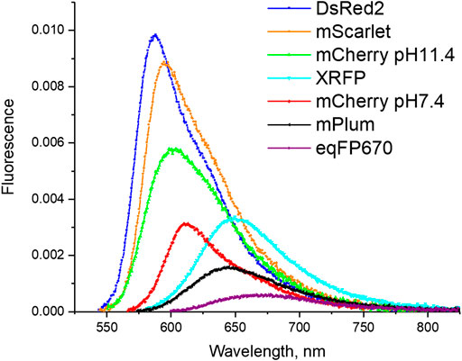
FIGURE 1. Fluorescence spectra of a set of RFPs studied in this work. The amplitude of the fluorescence intensity is normalized such that the integral under the curve is proportional to the fluorescence quantum yield.

Fast nonradiative relaxation leading to a low QY in the reddest variants of RFPs can be due to different mechanisms. First, the shift of the emission frequency of a molecule to the red (due to chemical modifications or interactions with environment) often results in acceleration of the internal conversion, following the “energy gap law” (Englman and Jortner, 1970; Jung et al., 2012). This mechanism is quite general and simply reflects the dependence of vibrational states distribution and coupling between them (through Franck-Condon factors) on the energy gap between the two electronic terms. Another mechanism of fast relaxation involves twisted intramolecular charge transfer (TICT) that becomes possible due to structural flexibility of the chromophore in some FP variants. In this case, the rotation about one or both of the bridge methine bonds (i.e., phenolate, P, or imidazolinone, I) drives the molecular system to a twisted state that corresponds to a conical intersection of the excited and ground states potential energy surfaces. Once in this state, the molecule undergoes an ultrafast transition from the excited to the ground state. Twisting in the excited state occurs in concert with significant charge transfer (CT) across the bridge from one side of the chromophore to another (Olsen and Smith, 2007; Simine et al., 2018; Park and Rhee, 2016; Sun et al., 2012, Moron et al., 2019).

In the isolated anionic GFP chromophore, such TICT states are quasi-stable intermediates on the excited state potential energy surfaces for either I- or P-rotations (Martin et al., 2004; Altoe et al., 2005). Those states are close to conical intersection seams, but still are separated from the ground state surface by small gaps (Martin et al., 2004; Altoe et al., 2005). In contrast, twisting of the isolated anionic RFP chromophore around the P-bond leads directly to a conical intersection seam at twisting angles of ∼75°–90° (Olsen and Smith, 2007). Like in the GFP chromophore, this rotation is virtually barrierless and exergonic. In contrast, twisting around the I-bond has a barrier and is endergonic. Olsen and Smith suggested that, in contrast to the GFP chromophore, in the RFP chromophore the electronegativity of the acylimine (A) substituent plays a decisive role in selecting the P-pathway of the TICT process.

As for the chromophore inside a protein, several factors can impede its ultrafast relaxation along the TICT pathway (Tolbert et al., 2012; Jung et al., 2012). Steric clashes with the surrounding bulky groups is the most obvious one. These interactions are usually much more efficient for rotation around the I-bond and less so for the P-bond (Chudakov et al., 2003; Stiel et al., 2008) because of the larger moving volume in the former case. A volume-conserving hula-twist motion involving concert rotation around both exocyclic bonds was put forward to explain low quantum yields in some GFP mutants (Jung et al., 2005) and the RFP mPlum (Moron et al., 2019), although this mechanism was questioned for GFP in (Altoe et al., 2005).

The effect of electrostatic interactions of the chromophore with the protein surrounding (including hydrogen bonding) can also contribute to the dynamics of TICT. In one scenario, a stronger electric field directed from P to I would shift the phenolate π-conjugation resonance from a quinonoid to a benzenoid form. This would facilitate rotation around the P-bond because it becomes closer to single in character. This so-called electronic effect of controlling nonradiative relaxation was experimentally observed in certain GFP mutants. Variants having less hydrogen bonding of the phenolate oxygen (i.e., more quinonoid structure) generally showed an increased quantum yield and fluorescence lifetime compared to mutants with more hydrogen bonds (benzenoid structure) (Jung et al., 2005; Jung et al., 2012). Alternatively, if the charge transfer corresponding to a shift of electronic density from P to I upon P-rotation is a more important factor than the bond order, than applying the field from I to P would speed up the rotation through an electrostatic driving force. This particular mechanism was theoretically predicted for GFPs (Park and Rhee, 2016; Simine et al., 2018) and RFPs (Olsen and Smith, 2007; Sun et al., 2012; Moron et al., 2019), however, it was not experimentally confirmed yet. Thus, it is crucial to experimentally measure the protein internal field. Such measurements however present a serious challenge, especially in the case of the two-dimensional RFP chromophore, in which both components of the field E projected onto the molecular axes (E_x and E_y) can be important.

In general, any of the above mechanisms, including vibrational relaxation described by the energy gap law and chromophore twisting (possibly sensitive to the electric field) can contribute to a fast nonradiative relaxation in RFPs (Figure 1). Our goal is to understand which of these processes is most important, if any. To this end, we need to evaluate the electric fields created by the protein environment at the chromophore site. A correlation (or the absence of one) between the nonradiative relaxation rate (k_nR) and the amplitude and direction of the local electric field for a set of RFP variants can reveal the mechanism of relaxation. Is a redder shift inextricably connected to a faster nonradiative relaxation? We aim to answer this important question, and, eventually, reveal clues as to how to find RFP variants with large quantum yields.

Materials and Methods

Identification and Cloning of XRFP

XRFP was identified as part of a large survey of published raw mRNA-Seq data sets in the NCBI Sequence Read Archive (SRA) database. Transcriptomes were assembled using Trinity (Grabherr et al, 2011; Haas et al., 2013) and using the public Galaxy bioinformatics server (Afgan et al., 2018). Candidate FP-encoding transcripts were identified by BLAST homology searching using avGFP as the query against the assembled transcriptome database. For each FP homolog found, the coding region was identified and a synthetic gene was designed to produce the encoded polypeptide sequence using codons optimized for Escherichia coli expression using an in-house BioXP3200 instrument (SGI-DNA, La Jolla, CA) or ordered as a gBlock double-stranded gene fragment (Integrated DNA Technologies, San Diego, CA). Fragments encoding FPs were inserted using Gibson assembly (Gibson et al., 2009) into the vector pNCS for expression (see below). XRFP was identified along with green- and orange-emitting FPs from the animal (data not shown).

Expression and Purification of Proteins

His-tagged RFPs were expressed in DH10B E. coli cells with bacterial expression plasmids encoding each protein. mScarlet, eqFP670, and mCherry were encoded on the pNCS vector, which contains a promoter for constitutive expression. DsRed2 and mPlum were encoded on pBAD; DsRed2-pBAD was a gift from Michael Davidson (Addgene plasmid # 54608; http://n2t.net/addgene:54608; RRID:Addgene_54608), and mPlum-pBAD was a gift from Michael Davidson and Roger Tsien (Addgene plasmid # 54564; http://n2t.net/addgene:54564; RRID:Addgene_54564). Escherichia coli expressing the RFPs were cultured in Circlegrow (MP Biomedicals) for 1–2 days at 30°. To induce expression of the pBAD plasmids, 0.1% w/v of L-arabinose was added to the media before inoculating. The fluorescent E. coli pellets were lysed with BugBuster (MilliporeSigma). Lysates were purified either with Ni-TED columns as per manufacturer’s protocol (Macherey–Nagel) or His60 Ni Superflow Resin (Clontech). For the latter, protein bound to the resin was washed 2–3 times with equilibration buffer (50 mM sodium phosphate, 300 mM sodium chloride, 20 mM imidazole; pH 7.4) ∼10 times the resin volume. Proteins purified via Ni-TED columns were eluted with buffer composed of 50 mM sodium phosphate, 300 mM sodium chloride, 250 mM imidazole; pH 8. For the His60 Ni Resin method, the elution buffer was 50 mM sodium phosphate, 300 mM sodium chloride, 300 mM imidazole; pH 7.4. Photophysical measurements were performed in elution buffer, except for mCherry pH 11.4, which was dialyzed into 25 mM sodium phosphate.

Linear Absorption and Fluorescence Properties

Linear absorption spectra were measured with a Lambda 950 spectrophotometer (Perkin Elmer). To obtain the peak extinction coefficient of an anionic chromophore, we performed a stepwise alkaline titration up to complete denaturation of the protein. At each step, 10 μl of 0.1 M NaOH was added to 0.5 ml of protein solution, held in a spectroscopic cuvette with 1-cm optical path, followed by recording of absorption spectrum. To correct for different protein concentrations at each step, absorption spectrum was multiplied by a factor equal to the ratio of total volume to initial volume of solution. Usually a dependence of optical density of the native anionic chromophore peak versus optical density of the denatured protein peak (at 452 nm) shows a linear region. In this region of pH, there are only two species present: the anionic chromophore in native protein and denatured protein (in the same region the series of absorption spectra show an isosbestic point). The slope of this linear dependence is equal to the ratio of extinction coefficients of the two species. Using known extinction value of denatured protein, 44,100 M⁻¹ cm⁻¹ at 452 nm (Ward, 2005; Gross et al., 2000), we obtain the extinction coefficient of anionic species. In the cases where the immature green chromophore was present initially, its contribution to the final denatured protein concentration was subtracted.

Corrected fluorescence spectra and fluorescence quantum yields were measured with an integrating sphere fluorometer (Quantaurus-QY, Hamamtsu) using 1-cm quartz cuvettes. The peak OD of the samples was <0.1. The reference (buffer-only) measurements were done in the same cuvette.

Fluorescence lifetime was measured with a Digital Frequency Domain system ChronosDFD (ISS) appended to a PC1 ISS spectrofluorometer. Peak optical density of the samples and reference solutions in 1-cm cuvettes was kept below 0.1. Fluorescence was excited with a 518-nm laser diode (ISS, model 73292). The excitation was modulated with multiple harmonics in the range 10–300 MHz for eqFP670 and mPlum, and 5–150 MHz for the rest of the proteins. In this method, a fluorescence lifetime standard is used to obtain the instrumental response function in each individual measurement. For cross checking, we employed Rose Bengal (Sigma-Aldrich) in ethanol with τ = 0.78 ns (Fleming et al., 1977; Cramer and Spears, 1978) or methanol, τ = 0.55 ns, (Fleming et al., 1977; Cramer and Spears, 1978; Reed et al., 1981; Rodgers, 1981, Lakowicz et al., 1986); Rhodamine 6G in deionized water, τ = 4.0 ns (Reisfeld et al., 1988; Magde et al., 2002; O’Hagan et al., 2001); and Rhodamine B in deionized water, τ = 1.74 ns (Boens et al., 2007). For each RFP, we used two or three different standards and the results were similar (deviations <6%). Fluorescence of all the samples and standards was collected at 90° through two identical 561LP Edge Basic^TM filters (Semrock) to cut off all excitation light. In the case of eqFP670 and mCherry (pH7.4), we used an additional HQ 650/20 (Chroma) filter to selectively collect fluorescence from the red-shifted form. For mCherry at pH 11.4, we used an additional HQ 577/10 filter (Chroma) to selectively collect fluorescence of the blue-shifted form. All the modulation ratio and phase delay curves were fitted to model functions corresponding to a single exponential fluorescence decay. The corresponding χ² values were in the range from 0.53 to 1.16.

Corrected fluorescence excitation spectra were obtained with a LS-55 spectrofluorimeter (Perkin Elmer). For mCherry at pH 11.4, the registration wavelength was 575 nm, where the red-shifted form does not fluoresce. For all other proteins, the registration wavelength was selected at the red side of the fluorescence spectrum near its maximum.

Two-photon Absorption Spectra, Cross Sections, and Polarization Ratio

Two-photon excitation spectra and cross sections were measured as described previously (Drobizhev et al., 2020). Briefly, we used an Insight DeepSee femtosecond laser (Spectra Physics) tunable in the 680–1,300 nm range coupled with a PC1 photon counting spectrofluorometer (ISS). LDS 798 in CDCl₃:CHCl₃ (2:1) solution was used as a spectral shape standard and Rhodamine 6G in MeOH was used as a 2PA cross section standard, with σ₂ = 10 GM at 1060 nm. The laser beam was focused into the sample with a NIR achromatic lens, f = 45 mm (Edmund Optics). The sample solutions were held in 3-mm spectroscopic cuvettes (Starna) and fluorescence was collected from the first 0.7-mm layer of solution, to avoid laser absorption by the solvent. A 745SP filter (Semrock) was placed after the sample to cut the scattered light. For mCherry pH 11.4, an additional HQ 577/10 filter (Chroma) was used.

To evaluate the two-photon polarization ratio Ω, the same experimental system was used. Additionally, a quarter-wave plate (Thorlabs) was placed in front of the entrance diaphragm of the fluorometer and the Glan polarizer (ISS) was set after the sample in the detection optical path. The quarter-wave plate was mounted on a rotation stage (Thorlabs) which made it possible to rotate it around both the laser propagation direction and the vertical axis. This helped to adjust the rotation and tilt angles to make the polarization very close to circular at each laser wavelength. The ellipticity of polarization was <7% in the tuning range 900–1,300 nm. By definition, Ω is the ratio of 2P cross sections obtained under circular and linear polarization of excitation. Experimentally, we collect fluorescence at 90° to excitation, first using circularly polarized light and then linearly (vertically) polarized light. To get rid of the effect of fluorescence polarization, at each polarization of laser, two measurements were done: one with the detection polarizer set vertically, and another with the detection polarizer set horizontally. The two-photon polarization ratio was then calculated as follows (Wan and Johnson, 1994):

$\text{Ω}=\frac{2F_{\text{OV}}+F_{\text{OH}}}{F_{\text{VV}}+2F_{\text{VH}}},(1)$

where F is the fluorescence signal, indexes O and V describe circular and vertical polarizations of excitation, respectively, and indexes V and H describe vertical and horizontal positions of detection polarizer. The sensitivity of the detector (PMT R928) for vertical versus horizontal polarization of fluorescence was checked by exciting the sample with horizontally polarized laser light and the ratio of the two signals (G-factor) was G = 1.0. Standard deviations of Ω were estimated from 10 measurements of Ω in the same conditions at a number of different wavelengths.

Molecular Dynamics Simulations

MD Parameters

Force field parameters for the mCherry, mPlum, and DsRed chromophores were those published in (Dmitrienko et. al., 2006) with the exception of excluding the phenolic hydroxyl hydrogen in order to form the anionic chromophore.

The optimized potentials for liquid simulations (OPLS) amino acid atom types suggested by Dmitrienko et. al. were also used. Standard OPLS-AA atom types were used for the extended chain atoms. A variant of the mCherry chromophore residue force field was also constructed, wherein equilibrium bond lengths and angles of the force field were set to those found in the 2H5Q pdb crystal structure rather than those suggested by Dmitrienko et al. for the neutral DsRed chromophore.

For both the DsRed and mCherry/mPlum chromophores, hydrogen addition rules were added to the OPLS-AA force field in such a way as to complete typical valency requirements for the anionic chromophores.

Simulation Details

All MD simulations were done with Gromacs-5.0.2 (Pronk et al., 2013). Initial atomic charges were found by protonating the pdb structure of a given mFruit protein using Gromacs, embedding it in a box of transferable intermolecular potential with 3 points (TIP3P) solvent, adding sodium ions in sufficient number to balance the charge of the protein, and then subjecting the chromophore to a semi-empirical INDO/S2 (ZINDO) analysis in the presence of the electric field due to non-chromophore protein atoms, water molecules, and ions in the simulation cell. Initial charges were calculated in this way for mCherry, mPlum, and DsRed, with a separate initial charge set determined for mCherry with its Glu215 residue protonated.

Following determination of an initial set of atomic charges for each mFruit protein chromophore based on the electrostatic environment, simulations were carried out. Each protein/simulation was treated with 100 ps of equilibration under the NVT ensemble with the protein heavy atoms constrained by a large harmonic restoring force, followed by 400 ps of NPT equilibration using the Berendsen barostat and a further 500 ps using the Parrinello-Rahman barostat, also with heavy protein atoms constrained. Finally, protein constraints were removed and 100 ns of dynamics was carried out, with positions saved each picosecond for a total of 100001 frames. The simulation was split into individual coordinate files, which were used for all subsequent analysis.

For each simulation frame a ZINDO calculation was performed, which yielded excitation energy, wavelength, oscillator strength, transition dipole, and Δμ for the 59 lowest energy transitions. All atoms in the simulation cell that were not part of the quantum chromophore were used to calculate the electric field vector and electric potential at each chromophore atom, so that the electrostatic environment could be completely accounted for in the ZINDO calculation. The output of the ZINDO calculations was also used to determine the S₀ and S₁ state charges for each simulation frame. The S₁–S₀ charge differences for each simulation were averaged, and those average values were used along with the atomic coordinates for each simulation frame to calculate the shift in chromophore excitation energy due to each protein atom that was not part of the quantum chromophore as well as for each water molecule and ion. This straightforward Coulombic summation allowed for the unambiguous assignment of Stark shifts due to protein, water and ions for each simulation frame as well.

Following the first set of 100 ns simulations based on initial MD charges, S₀ charge values for each quantum chromophore atom were plotted to assess charge convergence. The initial charges based on the solvated pdb structures were found to be quite close to those calculated for the chromophore during dynamics but were sufficiently different to warrant a second charge iteration. Average charge values for each MD chromophore atom were extracted from the above described plots, with an attempt made to identify portions of the trajectory where a given charge appeared to be approximately constant. These new MD chromophore atom charge values were used to begin a second set of 100 ns simulations of each RFP. Data for each simulation was analyzed using the ZINDO technique as described above, and chromophore charges during dynamics were found to be in excellent agreement with the static, assigned, second generation MD charges. After the 100 ns second charge iteration simulations, dynamics were continued for another 100 ps with frames collected every 2 fs. This high resolution data was analyzed in the same fashion as the coarser data sets described above.

Results

Role of Radiative and Nonradiative Relaxation Rates in Controlling Fluorescence Quantum Yield

We selected seven RFPs with a large variation of absorption/fluorescence peak wavelengths and fluorescence quantum yields. They include DsRed2 (Yanushevich et al., 2002), mCherry (Shaner et al., 2005) in pH 7.4 and in pH 11.4 buffers, having different electrostatic environment of chromophore (Shu et al., 2006), mPlum (Wang et al., 2004), mScarlet (Bindels et al., 2017), eqFP670 (Shcherbo et al., 2010), and XRFP (Shaner, 2018). Unless stated otherwise, all proteins were measured in a pH 7.4 buffer. With respect to the wild type DsRed (Matz et al., 1999), DsRed2 contains the R2A, K5E, K9T, V105A, I161T, and S197A mutations (Yanushevich et al., 2002). The optical properties of DsRed2 are very similar to DsRed (Drobizhev, et al., 2011) and, therefore, we will use the previously obtained data for DsRed as a reference, wherever possible. For consistency, we performed new independent measurements of the absorption and fluorescence photophysical properties of these proteins, Table 1.

TABLE 1

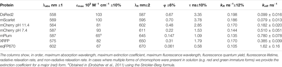
TABLE 1. Absorption and fluorescence properties of RFPs.

Since the extinction coefficient does not change very much in the series, the key parameter determining molecular brightness (ε_maxφ) is the fluorescence quantum yield (φ). The quantum yield decreases about an order of magnitude when going from DsRed2 and mScarlet to the most red-shifted variant eqFP670, Table 1. The quantum yield and fluorescence lifetime depend on both the radiative relaxation rate (k_R) and nonradiative relaxation rate (k_nR):

$\phi =\frac{k_R}{k_R+k_{nR}},(2)$

$\tau =\frac{1}{k_R+k_{nR}}.(3)$

To understand the role of k_R and k_nR in controlling quantum yield, we calculated them from the measured φ and τ,

$k_R=\frac{\phi }{\tau },(4)$

$k_{nR}=\frac{1-\phi }{\tau } ,(5)$

and present them in Table 1. The dependence of k_R on the cube of fluorescence peak frequency, ${\overline{\nu }}_f$ (in cm⁻¹), is shown in Figure 2. The dashed line is a linear fit representing the Einstein coefficient for spontaneous emission as a function of ${\overline{\nu }}_f^3$,

$k_{R }=\frac{4{\left(2\pi \right)}^4{n}^3}{3h}{\mu }_{em}^2{\overline{\nu }}_f^3.(6)$

Here n is the refractive index of the medium and h is the Planck constant. The slope of the fit is proportional to the matrix element of the transition dipole moment squared μ_em². The slope provides an average transition dipole moment, ǀμ_emǀ = (7.1 ± 0.2) D. In general, the k_R value does not change more than twofold in the series. On the other hand, k_nR varies about 20 times; see Table 1. We thus conclude that k_nR plays a decisive role in controlling quantum yield.

FIGURE 2

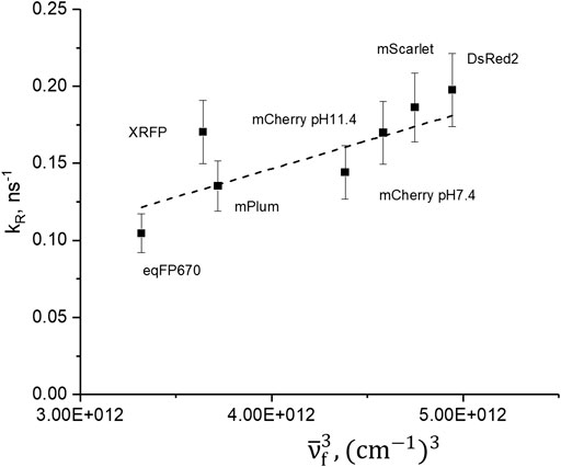
FIGURE 2. Dependence of radiative relaxation rate on cube of maximum fluorescence frequency. Dashed line represents the best fit to the Einstein equation for spontaneous emission rate.

Checking the Energy Gap Law

The energy gap law predicts an exponential decrease of k_nR with the increase of the energy gap ΔE for fluorescence transition between the energy levels of S₁ and S₀ states (Englman and Jortner, 1970):

$k_{nR }=C\exp \left(-\frac{\xi \Delta E}{h{\nu }_M}\right),(7)$

where C is a constant factor, ξ is a parameter that only slowly varies with ΔE and ν_M is the maximum molecular normal vibration frequency (in Hz). Figure 3 shows the dependence of nonradiative relaxation rate (in logarithmic scale) on the fluorescence peak frequency ${\overline{\nu }}_{\text{f}}=\text{ Δ}E/\text{c}h$ for the series of RFPs studied here (red circles).

FIGURE 3

FIGURE 3. Dependence of nonradiative decay rate (log scale) on peak fluorescence frequency. Red circles correspond to RFPs studied here and green triangles correspond to a number of GFPs variants, studied previously (Drobizhev et al., 2011; Molina et al., 2017). The dashed lines represent linear fits to the two sets of data.

Although the RFPs qualitatively follow the predicted dependence Eq. 7, the correlation is not very strong (Pearson’s R = −0.858). In particular, although the peak fluorescence frequencies of mScarlet and mCherry pH 11.4 are very close, their k_nR values differ more than twofold, a difference much larger than the experimental errors. This is similarly true for the XRFP and mPlum pair. These quantitative inconsistencies suggest that the internal conversion through vibrionic coupling between S₁ and S₀ states, reflected in the energy gap law, is probably not the dominant mechanism of relaxation. Another, indirect support for a failure of this mechanism is obtained by considering the behavior of k_nR in a series of proteins with green anionic chromophore, shown in Figure 3 by green triangles. The mutants and homologues of GFP of this series were characterized previously (Drobizhev et al., 2011; Molina et al., 2017). They were selected such that they all have high quantum yields, 0.67–0.91, (to exclude other possible deactivation mechanisms, e.g., twisting around the bridge bonds), and their fluorescence spectra span a broad range, from 482 (Rosmarinus) to 537 nm (phiYFP). Due to a close similarity in the structures of the green and red chromophores, as well as closeness in shape of the absorption and fluorescence spectra in the two series, one would expect that the energy gap law, if dominant in controlling k_nR, would be observed in both series. However, the “green” set does not show any correlation between k_nR and ${\overline{\nu }}_{fl}$. We therefore conclude that the energy gap law is not a main mechanism of relaxation in the studied set of RFPs (and GFPs) and will consider alternative mechanism in Section “Describing the Rate of TICT Process with Marcus Formalism”. To this end, we must first investigate the internal electric field created by the protein at the chromophore site.

Physical Model for Determining the Protein Internal Electric Field at the Chromophore Site

The protein surrounding the chromophore creates an internal electric field that may play an important role in the mechanism of nonradiative relaxation. To determine the components of this field in the plane of the chromophore, we developed a physical model based on the following assumptions: 1) The local electric field does not change neither upon electronic excitation of the chromophore (environment is polarizable only in the ground state) nor upon twisting around exocyclic P-bond in the excited state. 2) The potentially non-homogeneous field varying from one atom to another on the chromophore will produce the same effect as a homogeneous effective field E. The first assumption was recently proven to a first approximation for DsRed (List et al., 2012) and a series of GFP variants (Nifosi et al., 2019). The effective field obtained after averaging the fields on several atoms of the chromophore’s π-conjugation system was also shown to describe optical properties reasonably well (Nifosi et al., 2019).

In our approach of evaluating the local electric field, we use the permanent dipole moment of the chromophore μ^(g,e), where indices g and e correspond to the ground and excited states, respectively, as a linear metric of the field. In fact, if an electric field of a large magnitude (|E| ∼10⁷–10⁸ V/cm) is applied to a dipolar molecule with nonzero polarizability α, its dipole moment μ^(g,e) will acquire an additional, induced, part equal to μ^(g,e)_ind = $\underset{¯}{\alpha }$E comparable to the vacuum dipole moment μ^(g,e)₀. (The underline denotes the tensorial nature of polarizability.) Experiments and calculations show that such strong fields are indeed present in proteins (Geissinger et al., 1995; Manas et al., 1999; Schweitzer-Stenner, 2008; Callis and Burgess, 1997; Vivian and Callis, 2001). Therefore, for the linear in the field approximation, the total dipole moment reads (Atkins and Friedman, 1997):

${\mu }^{(g,e)}={\mu }_0^{(g,e)}+ {\underset{¯}{\alpha }}^{(g,e)} E.(8)$

For simplicity, we consider the chromophore to be planar in the ground electronic state, although small twist and tilt angles are present in some RFPs (Shu et al., 2006). We also assume here that μ^(e) and ${\underset{¯}{\alpha }}^{\left(e\right)}$ correspond to an excited state with positions of the atomic nuclei unchanged compared to the ground state. Applying Eq. 8 separately to the ground and the excited state and then subtracting the former from the latter, we obtain:

$\Delta \mathit{\mu }=\Delta {\mathit{\mu }}_0+\Delta \underset{¯}{\alpha }\mathit{E}(9)$

We now select x and y coordinate axes such that they correspond to the main axes of the 2x2 tensor of the polarizability change, Δα, i.e., the frame where it is diagonal with components Δα_xx and Δα_yy. In the same coordinate frame, the Δμ = μ^(e)− μ^(g) vector has components Δμ_x and Δμ_y; Δμ_0,x and Δμ_0,y are the components of Δμ₀. Equation 9 can be projected onto the x and y coordinate axes resulting in

$\text{Δ}{\mu }_x=\text{Δ}{\mu }_{0,x}+\text{Δ}{\alpha }_{xx}{E}_x,(10)$

$\text{Δ}{\mu }_y=\text{Δ}{\mu }_{0,y}+\text{Δ}{\alpha }_{yy}{E}_y.(11)$

(Note that in our previous papers (Drobizhev et al., 2009; Drobizhev et al., 2012a) the coefficient ½ was used in the second term of the right-hand side of Eq. 9 following an erroneous presentation in some previous literature, see e.g. (Berlin et al., 2006). A correct formula (Atkins and Friedman, 1997) does not contain it.)

If Δμ_x and Δμ_y were known, then it would be possible to calculate the field components E_x and E_y , by solving Eqs 10, 11:

$E_x=\frac{\Delta {\mu }_x-\Delta {\mu }_{0,x}}{\Delta {\alpha }_{xx}},(12)$

$E_y=\frac{\Delta {\mu }_y-\Delta {\mu }_{0,y}}{\Delta {\alpha }_{yy}}.(13)$

Now, we will demonstrate how to obtain Δμ_x and Δμ_y values for a chromophore within a protein, using one- and two-photon absorption spectroscopy. In our method we also rely on the quantum-mechanically calculated parameters of the isolated chromophore: transition frequency, ${\overline{\nu }}_0$, and components of polarizability tensor, Δα_xx and Δα_yy, and dipole moment vector, Δμ_0,x and Δμ_0,y. This approach allows us to limit the size of the molecular system that has to be calculated quantum-mechanically to the chromophore group. We can then evaluate the parameters sensitive to the protein environment purely from experiment.

Two experimental values have to be measured in the region of the pure electronic S₀ -> S₁ transition: 1) the one-photon absorption frequency $\overline{\nu }$ and 2) the change of the permanent dipole moment upon excitation, Δμ = |Δμ|. (Here and throughout we call the pure electronic, or 0–0, transition, the one that does not involve excitation of high frequency vibrations, ${\overline{\nu }}_v$ > 1,000 cm⁻¹). The first value can be obtained from the one-photon absorption (1PA) spectrum. The second requires the two-photon absorption (2PA) spectrum in absolute cross-section values, as well as the two-photon polarization ratio (i.e., the ratio of fluorescence signals obtained upon circular and linear two-photon excitation).

Due to the Stark effect, the chromophore experiences a spectral shift of its one-photon absorption transition frequency from ${\overline{\nu }}_0$ in vacuum to $\overline{\nu }$ inside the protein. Since we are dealing with strong fields such that Δμ itself depends on the field, we should include the quadratic terms in the field dependence (quadratic Stark effect). The optical transition energy for the chromophore in protein will read (Atkins and Friedman, 1997):

$hc\overline{\nu }=hc{\overline{\nu }}_0-\text{Δ}{\mu }_{0,x}{E}_x-\text{Δ}{\mu }_{0,y}{E}_y-\frac{1}{2}\text{Δ}{\alpha }_{xx}{E}_x^2-\frac{1}{2}\text{Δ}{\alpha }_{yy}{E}_y^2.(14)$

We use the e.s.u. system of units here and throughout, unless specified otherwise. Frequency $\overline{\nu }$is expressed in cm⁻¹, h is the Planck constant, and c is the speed of light in vacuum. Substituting Eq. 12 and Eq. 13 into Eq. 14, we obtain the relation between the transition energy and the Δμ_0,x, Δμ_0,y, Δμ_x, and Δμ_y components:

$hc\overline{\nu }=hc{\overline{\nu }}_0+\frac{\text{Δ}{\mu }_{0,x}^2}{2\text{Δ}{\alpha }_{xx}}+\frac{\text{Δ}{\mu }_{0,y}^2}{2\text{Δ}{\alpha }_{yy}}-\frac{\text{Δ}{\mu }_x^2}{2\text{Δ}{\alpha }_{xx}}-\frac{\text{Δ}{\mu }_y^2}{2\text{Δ}{\alpha }_{yy}}.(15)$

To find Δμ_x and Δμ_y, it is convenient to re-group Eq. 15 as follows:

$\frac{\text{Δ}{\mu }_x^2}{\text{Δ}{\alpha }_{xx}}+\frac{\text{Δ}{\mu }_y^2}{\text{Δ}{\alpha }_{yy}}=\frac{\text{Δ}{\mu }_{0,x}^2}{\text{Δ}{\alpha }_{xx}}+\frac{\text{Δ}{\mu }_{0,y}^2}{\text{Δ}{\alpha }_{yy}}-2hc(\overline{\nu }-{\overline{\nu }}_0).(16)$

Equation 16 represents a conic section in the (Δμ_x, Δμ_y) coordinate plane, which, depending on the signs of Δα_xx and Δα_yy, could be either an ellipse or a hyperbola (if Δα_xx ≠ Δα_yy). The curve is fully determined if the value of $\overline{\nu }$ is measured and Δμ_0,x, Δμ_0,y, Δα_xx, Δα_yy, and ${\overline{\nu }}_0$ are calculated quantum mechanically.

The second equation for finding the Δμ_x and Δμ_y components comes from the expression of the 2PA cross section, deduced from the second order perturbation theory in the two-level approximation of the S₀ → S₁ transition (Drobizhev et al., 2009) for linearly polarized degenerate excitation. The two-level approximation was justified by quantum mechanical calculations for the RFP chromophore (Drobizhev et al., 2009). The 2PA cross section corresponding to the pure electronic peak, σ₂(0–0), depends on several factors. These are: Δμ², the extinction coefficient ε(0–0) (in M⁻¹ cm⁻¹), transition frequency $\overline{\nu }$ (we assume that the one-photon absorption peak coincides with the 0–0 transition), and γ, the angle between the transition dipole moment μ and the change of the permanent dipole moment Δμ :

${\sigma }_2\left(0-0\right)=A\frac{\text{Δ}{\mu }^2\epsilon (0-0)(1+2co{s}^2\gamma )}{\overline{\nu }},(17)$

where the factor A is equal to

$A=\frac{4 {10}^3\pi \ln 10f_{\text{opt}}^2}{5h{c}^{2}n{N}_A} .(18)$

Here, N_A is the Avogadro’s number, f_opt is the local field factor at optical frequency $\overline{\nu }/2$, which is usually assumed to be of a Lorentz form (Bloebmergen, 1965): f_opt = (n²+2)/3.

The angle γ can be obtained experimentally by comparing the 2PA cross sections measured under circularly $\left({\sigma }_2^{\mathrm{\circlearrowleft }}\right)$ and linearly $\left({\sigma }_2^{\updownarrow }\right)$ polarized light. Within the two-level approximation of the degenerate 2PA process, the ratio of the two measurements Ω depends on γ as follows (Meath and Power, 1984):

$\Omega =\frac{{\sigma }_2^{\mathrm{\circlearrowleft }}}{{\sigma }_2^{\updownarrow }}=\frac{{\cos }^2\gamma +3}{4{\cos }^2\gamma +2}.(19)$

As one can see, the polarization ratio spans the range between 2/3 and 3/2 when γ varies from 0° to 90°. Solving Eq. 19 for γ results in

$\gamma =\pm \arccos \sqrt{\frac{2\left(1-\Omega \right)}{4\Omega -1}}+\pi n; n=\mathrm{0,1,2},\dots (20)$

Solving Eq. 17 for Δμ² and noticing that ${\left|\text{Δ}\mu \right|}^2= \text{Δ}{\mu }_x^2+\text{Δ}{\mu }_{\text{y}}^2$, we get

$\Delta {\mu }_x^2+\Delta {\mu }_y^2= \frac{{\sigma }_2\left(0-0\right)\overline{\nu }}{A\epsilon \left(0-0\right)\left(1+2{\cos }^2\gamma \right)}.(21)$

Equation 21 presents a circle in the (Δμ_x, Δμ_y) coordinate plane with the radius equal to

$\left|\Delta \mu \right| =\sqrt{\frac{{\sigma }_2\left(0-0\right)\overline{\nu }}{A\epsilon \left(0-0\right)\left(1+2{\cos }^2\gamma \right)}} .(22)$

The curve Eq. 21 is fully determined if the values of $\overline{\nu }$, σ₂(0−0), ε(0−0), and γ are measured and the constant A is calculated according to Eq. 18. Generally, the system of two conical sections Eq. 16 and Eq. 21 can have up to four possible solutions for the vector Δμ = (Δμ_x, Δμ_y). In Section “Electric Fields in RFPs” we will show how independent knowledge of the direction of the transition dipole moment in the molecular frame, as well as MD simulations can help to select the right solution.

Parameters of the Isolated RFP Chromophore Calculated Quantum Mechanically

To obtain the Δμ_0,x, Δμ_0,y, Δα_xx, and Δα_yy values, we started from the available structure of the mCherry protein (Shu et al., 2006). We cut the chromophore group (residues 65 and 66 in 2H5Q pdb file) out of the protein, added the hydrogen atoms to it, and optimized its geometry using Gaussian 09 (Frisch et al., 2016) and the B3LYP/6-311++G(d,p) density functional and basis set (Figure 4, bottom). In the optimization process, we forced the I and P rings to lie in the same plane (i.e., flat chromophore). We performed geometry optimization for a chromophore in a set of electric field values applied separately along each axis, x and y. Molecular system of coordinates was selected such that the change of polarizability tensor $\Delta \underset{¯}{\alpha }$ is diagonal in it, as described before (Drobizhev et al., 2012a), see Figure 4, bottom. Using a version of Zerner’s INDO/S2-CIS (“ZINDO”) method (Ridley and Zerner, 1973) modified to add oxygen parameters suggested by the Truhlar group (Li et al., 1999) we calculated Δμ_x and Δμ_y at each value of the field for the vertical optical transition. (Note that the TD-DFT often underestimates the Δμ values (Jacquemin, 2016) and ZINDO performs better than TD-DFT in calculating the RFP chromophore photophysical properties (Schaefer et al., 2007)).

FIGURE 4

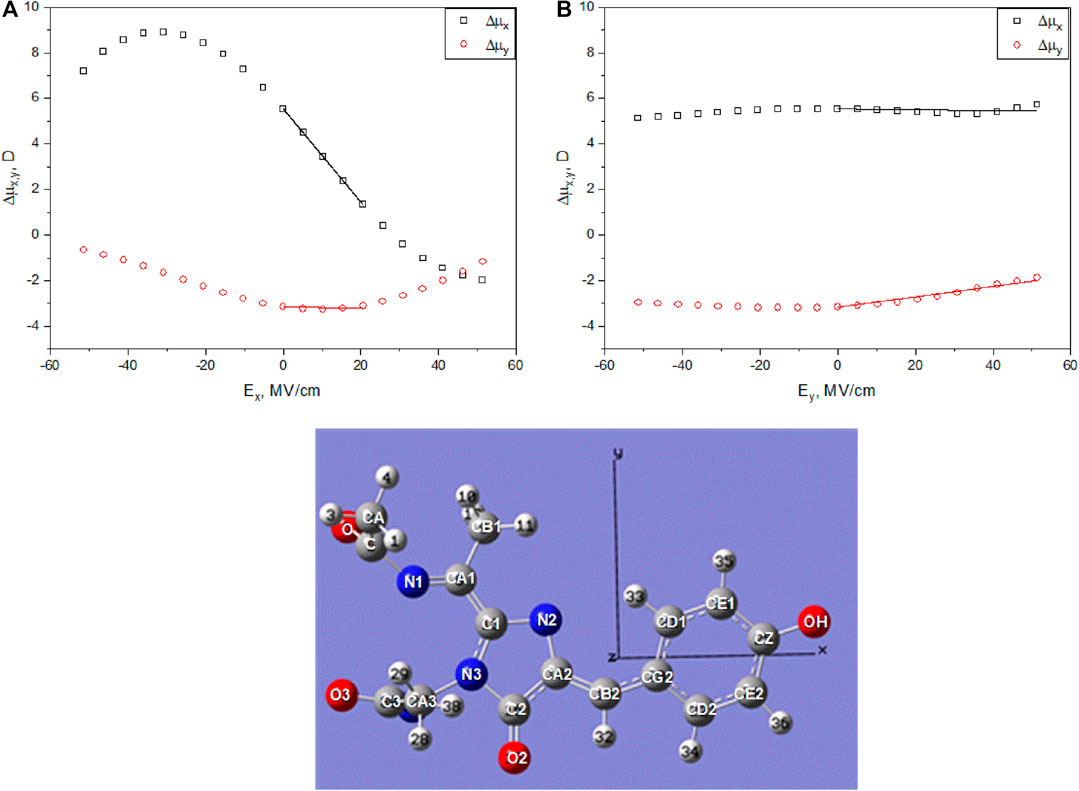
FIGURE 4. Top: Calculated permanent dipole moment differences, Δμ_x (black squares) and Δμ_y (red circles), between the excited and ground states of the RFP chromophore as function of applied electric field E_x(A) and E_y(B). In the calculations, the chromophore structure was optimized for each value of the field with the phenolate and imidazolinone rings constrained to lie in the same plane (flat chromophore). Bottom: Chromophore structure optimized at zero field with the directions of axes x and y shown.

Figure 4 shows the dependences of Δμ_x and Δμ_y on E_x (a) and E_y (b) obtained for the RFP chromophore in vacuum. We find that at zero field, Δμ_0,x = 5.53D and Δμ_0,y = −3.17D. The signs of the two components suggest that at least for the isolated chromophore, the electronic density shifts from P to I and also from I to A part upon excitation (by definition, the electric dipole moment is directed from negative charge to positive charge). The dependences of Δμ components on the field were fitted to linear functions (Eqs 10,11) in the ranges of the field E_x = 0 ÷ 20 MV/cm and E_y = 0 ÷ 50 MV/cm, typical for the set of RFPs studied here (vide infra) with fixed zero-field values Δμ_0,x and Δμ_0,y. The slopes of these regressions constitute the elements of the $\Delta \underset{¯}{\alpha }$ tensor: Δα_xx = −61.3 ± 0.2 ų and Δα_yy = 6.9 ± 0.3 ų. As expected, the main component of Δα is directed along the molecular axis encountering the greater number of π-electrons, i.e., the line connecting the centers of two π-conjugated rings. The minor component is due to the A part and/or parts of conjugated system of P and I extended in a direction perpendicular to x.

The vacuum transition frequency ${\overline{\nu }}_0$ of the red FP chromophore was previously obtained in (Taguchi et al., 2009) using fragment molecular orbital (FMO) calculations and the method of configuration interaction singles with perturbative doubles, including higher-order corrections and partial renormalization, i.e., PR-CIS(Ds). This method provided an excellent agreement between the theoretical and experimental transition frequencies for the RFP chromophore within proteins. The corresponding differences between the two were 0 cm⁻¹ for DsRed, −560 cm⁻¹ for mCherry, and 320 cm⁻¹ for mStrawberry. Transition frequencies of the isolated model chromophore with slightly different frozen conformations, corresponding to DsRed, mCherry, and mStrawberry geometry in low-temperature crystals, were calculated to be 15,890, 16,370, and 16,530 cm⁻¹, respectively. For our purposes we take the average value of these three: ${\overline{\nu }}_0$ = 16,260 cm⁻¹. We assume that it will represent well all possible conformational variations of the chromophore.

Finding Dipole Moment Difference Δμ and the Angle γ between the Vectors μ and Δμ

In this section we will find the absolute values of Δμ and the angle between μ and Δμ using one- and two-photon absorption spectroscopy. This information is necessary for evaluation of local electric fields, performed in Section “Electric Fields in RFPs”. The top panels of Figure 5 show one-photon absorption, fluorescence, and two-photon absorption spectra in the region of the S₀ –>S₁ transition of RFPs. We found that all the proteins studied here can be divided in two groups, according to their Stokes shifts values. DsRed2, mCherry, and mScarlet have smaller Stokes shifts (<1,200 cm⁻¹), and mPlum, XRFP, and eqFP670 have larger Stokes shifts (≥1,500 cm⁻¹). We assume that in proteins with larger Stokes shifts there are additional mechanisms of relaxation in the excited state.

FIGURE 5

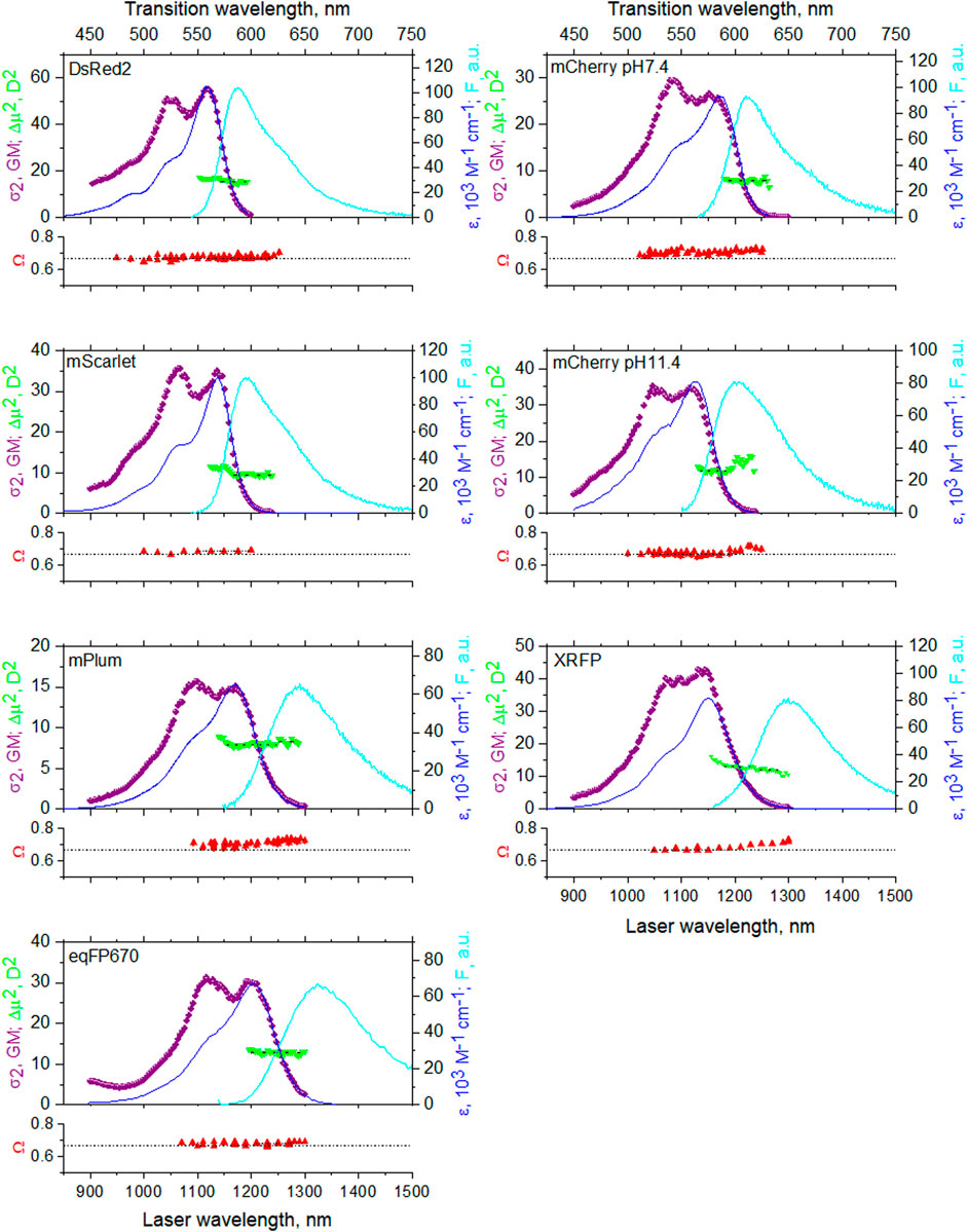
FIGURE 5. Top panels: one-photon absorption (dark blue line, right y-axis), fluorescence normalized to one-photon absorption peak (cyan line, right y-axis), and two-photon absorption (purple symbols, left y-axis) spectra in the region of the S₀ -> S₁ transition. Green triangles represent the calculated Δμ² values (left y-axis) as a function of excitation wavelength. Bottom panels show the two-photon polarization ratio Ω (red symbols) as a function of excitation wavelength. Horizontal dashed line represents a limiting case of Ω = 2/3, γ = 0. The top x-axis corresponds to transition wavelength, that is the same for both 1P and 2P excitation, and the bottom x-axis corresponds to laser wavelength, used for 2P excitation.

It is known that the absorption spectra of mCherry at pH 7.4 and pH 11.4 (Shu et al., 2006), mPlum (Wang et al., 2004), and DsRed (Matz et al, 1999) contain contributions from at least two different forms. In particular, the mCherry spectrum always contains two contributions, one dominating at acidic pH and another at alkaline pH. In addition to a major red peak, mPlum and DsRed display a shorter wavelength minor peak, corresponding to the immature green chromophore (Gross et al., 2000; Shu et al., 2006). Therefore, in Figure 5 we present absorption spectra in the form of corrected fluorescence excitation spectra scaled to extinction coefficient of the major form. These excitation spectra were measured with the fluorescence monochromator set at a wavelength where the contributions of the minor forms were negligible. The 2PA spectra were all measured in the form of fluorescence excitation spectra and scaled to the two-photon absorption cross section. In these measurements, we again selected the excitation of the main form by choosing the appropriate observation wavelength.

At the long-wavelength side of the pure electronic transition, the shapes of the 1PA and 2PA spectra perfectly match (when plotted against transition wavelength). This demonstrates that the pure electronic transition is simultaneously allowed for both one- and two-photon absorption and its broadening does not depend on the mode of excitation. This behavior is expected for dipolar chromophores, such as the one considered here. Differences in the 2PA and 1PA spectral shapes at shorter wavelengths, i.e., in the region of vibronic transitions, can be explained by the Herzberg–Teller contribution to the Δμ factor, present only in 2PA (Drobizhev et al., 2012b). Green downward triangles in the top panels represent the wavelength dependence of |Δμ|² calculated according to Eqs 18, 21 in the region of pure electronic transition from independently measured σ₂(0–0), ε(0–0), and γ.

The bottom panels of Figure 5 show the two-photon polarization ratio Ω as a function of wavelength. This value allows to calculate the angle γ. Analysis of the previous literature shows that the direction of transition dipole moment μ generally does not depend on the local environment in proteins with the same chromophore structure (List et al., 2012; Ansbacher et al., 2012; Nifosi et al, 2019, Myskova et al, 2020). On the other hand, the direction of Δμ is more sensitive to local electrostatics (see below). Therefore, we can consider Ω as a qualitative metric for the direction of Δμ within the chromophore coordinates. Furthermore, Ω can resolve spectrally overlapping transitions with different directions of Δμ. These transitions can belong to conformers with different structures of the chromophore environment creating different local electric fields.

For the proteins with a small Stokes shift (four upper graphs in Figure 5), Ω is virtually constant in the region 950–1,250 nm. This points to the presence of a single electronic S₀ –> S₁ electronic transition in this region, cf. (Masters et al., 2018). Ω values between 0.67 and 0.71 correspond to small γ angles in these proteins, Table 2. mCherry at pH 11.4 presents an exception, where Ω slightly increases from 0.67 to 0.71 when going from the main peak toward the very red tail of the spectrum at λ > 1200 nm. This can be due to a minor, red-shifted, form contributing to the fluorescence signal at the long excitation wavelengths (despite selective detection of fluorescence). This is probably the form that dominates the spectrum at neutral pH with a different electrostatic environment of the chromophore (Shu et al., 2006). In fact, mCherry at pH 7.4 shows Ω = 0.71 across most of the spectrum and its absorption is shifted to the red, peaking near 1,200 nm (Figure 5).

TABLE 2

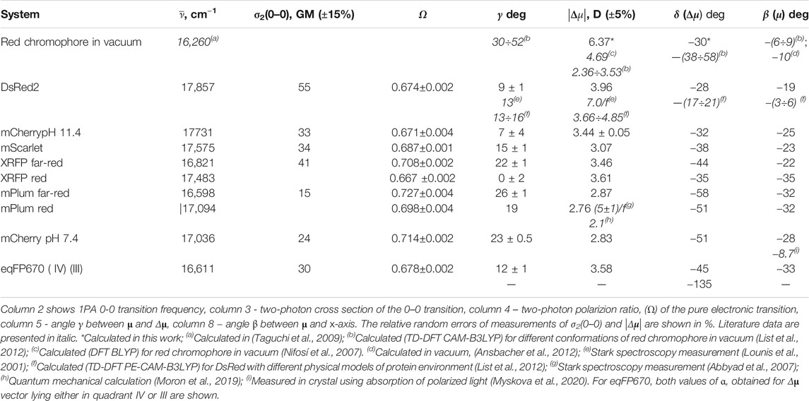
TABLE 2. Permanent dipole moment difference vector with its length |Δμ| and its direction (angle δ ) relatively to x-axis, as well as other parameters involved in finding Δμ.

For the proteins with a large Stokes shift (three bottom graphs in Figure 5), only eqFP670 displays a constant value of Ω across the spectrum. In mPlum and XRFP, Ω first increases and then reaches a plateau in the red tail of the 0–0 transition. Correspondingly, γ changes from 19° to 26° in mPlum and from 0° to 22° in XRFP. This suggests a presence of at least two different conformations of the chromophore environment in these proteins.

It is known that in mPlum a large Stokes shift of fluorescence is due to a fast reorganization of the chromophore environment in the excited state (Konold et al., 2014; Faraji and Krylov, 2015; Yoon et al., 2016). Specifically, a direct hydrogen bond between the acylimine oxygen of the chromophore and the E16 carboxyl oxygen of the protein reorganizes to a water-mediated hydrogen bond at the same site. This causes the chromophore to switch from a red emitting form to a far-red emitting form. Since the switch between the two forms occurs on a picosecond time scale, the far-red form dominates in steady-state fluorescence. On the other hand, a small fraction of the far-red form is present in the ground state and can be directly excited (Faraji and Krylov, 2015; Yoon et al., 2016). Our experiment supports this observation because Ω, being independent of emission transition dipole moment by definition (Wan and Johnson, 1994), points to the presence of a minor, far-red form in the ground state with a different direction of Δμ. The latter could be assigned to water-mediated hydrogen bonding at the acylimine oxygen. The spectral variation of Ω can be used to resolve the contributions of the two forms (we label the red and far-red forms a and b, respectively), similarly to the case of 1P fluorescence anisotropy measured as a function of excitation wavelength (Lakowicz, 2006). Using the property of additivity of Ω and assuming that both forms fluoresce with the same quantum yield φ_b because the red form rapidly converts to the far-red one in the excited state, we can write (Rehms and Callis, 1993):

$\Omega \left(\lambda \right)=f_a\left(\lambda \right){\Omega }_a+f_b\left(\lambda \right){\Omega }_b,(23)$

where f_a(λ) and f_b(λ) are the fractional contributions to the 2PA of the two forms. Specifically, $f_a\left(\lambda \right)= \frac{{\rho }_a{\sigma }_{2,a}\left(\lambda \right)}{{\rho }_a{\sigma }_{2,a}\left(\lambda \right)+{\rho }_b{\sigma }_{2,b}\left(\lambda \right)}$, and $f_b\left(\lambda \right)= 1-f_a\left(\lambda \right)$, where ρ_a and ρ_b are the fractional concentrations of forms a and b. Combining the last relation with Eq. 23, we can write:

$f_a=\frac{{\Omega }_b-\Omega \left(\lambda \right)}{{\Omega }_b-{\Omega }_a},(24)$

$f_b=\frac{\text{Ω}\left(\lambda \right)-{\text{Ω}}_a}{{\text{Ω}}_b-{\text{Ω}}_a},(25)$

where Ω_a = 0.698 and Ω_b = 0.730 are the corresponding pure Ω values found experimentally. The spectral contributions of the two forms to the total two-photon absorption spectrum, ${\sigma }_{2,total}\left(\lambda \right)= {\rho }_a{\sigma }_{2,a}\left(\lambda \right)+{\rho }_b{\sigma }_{2,b}\left(\lambda \right)$, are calculated as follows:

${\rho }_a{\sigma }_{2,a}\left(\lambda \right)=f_a\left(\lambda \right){\sigma }_{2,\text{total}}\left(\lambda \right),(26)$

${\rho }_b{\sigma }_{2,b}\left(\lambda \right)=f_b\left(\lambda \right){\sigma }_{2,\text{total}}\left(\lambda \right).(27)$

and are shown in Figure 6, top, together with the total 2PA spectrum.

FIGURE 6

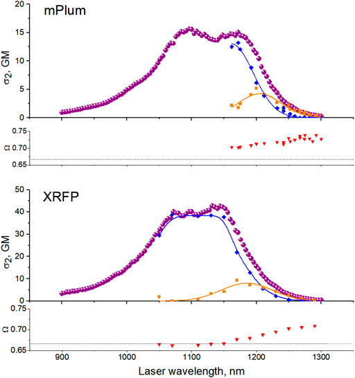
FIGURE 6. Resolution of two-photon transitions corresponding to two different conformations of the chromophore’s environment in mPlum (top) and XRFP (bottom). Top panels: Purple circles represent the total effective 2PA cross section ${\sigma }_{2,total}{\left(\lambda \right)}_a$, blue rhombs—contribution from the red from $\left({\rho }_a{\sigma }_{2,a}\left(\lambda \right)\right)$ and orange squares – from the far-red form $\left({\rho }_b{\sigma }_{2,b}\left(\lambda \right)\right)$. Bottom panels: Red triangles represent Ω values. The dashed line corresponds to the Ω = 2/3 (γ = 0) case.

Applying the same method to XRFP, we resolved its 2PA spectrum into two forms, Figure 6, bottom. In the case of eqFP670, the independence of Ω on excitation wavelength suggests that there is a single ground state conformation in the range of 1,200–1,300 nm. The large Stokes shift can still be tentatively explained by a conformational change of the chromophore’s environment in the excited state.

Table 2 summarizes the magnitude of vector Δμ, and the angles it makes with the vector μ (γ) and the x-axis (δ), as well as other spectroscopic parameters that we used to obtain this information. For comparison, the table also includes the calculated data for the chromophore in vacuum and relevant literature data. For mPlum and XRFP, where two forms were found in the absorption spectra, we provide a set of parameters for each form. The |Δμ| values were previously measured using Stark spectroscopy for DsRed and mPlum in frozen water/glycerol solution, up to a constant local field factor f (Lounis et al., 2001; Abbyad et al., 2007). Both of them are consistent with our data if we assume f = 1.75, which is in the range predicted in (Fried et al., 2013) for the frozen solutions, such as those used in Stark measurements. The angle γ = 13⁰ found for DsRed in (Lounis et al., 2001) using Stark spectroscopy is close to our value (9⁰). Our experimental value of |Δμ| for DsRed2 also agrees well with the quantum mechanical calculations (List et al., 2012) where different models were explored to describe protein environment. The |Δμ| values obtained for the red anionic chromophore in vacuum (Nifosí et al., 2007; List et al., 2012) with DFT calculations are lower than our semi-empirical calculation probably because the DFT often underestimates |Δμ| (Jacquemin, 2016).

Electric Fields in RFPs

A graphical representation of the curves described by Eqs 16, 21 in the Δμ_x, Δμ_y plane provides the solutions of this system of equations as the intersections of these two curves. Figure 7 plots the equations of the hyperbola Eq. 15 and the circle Eq. 21 for the DsRed2 protein, using the isolated chromophore parameters calculated in Section “Parameters of the Isolated RFP Chromophore Calculated Quantum Mechanically” and the experimental values of $\overline{\nu }$ and |Δμ| taken from Table 2. There are four possible solutions for Δμ found at the intersections of the red and blue curves in each of the quadrants I–IV. To resolve this ambiguity, we take into consideration the following two points. 1) The Δμ vector in DsRed protein was calculated (List et al., 2012) for a polarizable environment (PE-QM), a frozen polarizable environment (FPE) and a non-polarizable environment (NPE). The purple dashed arrows in Figure 7 correspond to these three cases. The angle between Δμ and the x-axis, calculated clockwise, increases in the order: PE-QM, FPE, and NPE, respectively. All three vectors are found in quadrant IV and are close to our experimental result obtained for quadrant IV (purple solid arrow). 2) The direction of the oscillating transition dipole moment μ was also calculated in (List et al., 2012), both for chromophore in vacuum and in protein with different models describing the environment. In all cases, the μ vector fell within the quadrants II and IV and made an angle β = −(3–9)° with the x-axis, Figure 7, showing that the protein environment did not affect it much. The direction of μ in an isolated RFP chromophore, optimized in vacuum, was also calculated in (Ansbacher et al., 2012) with a result similar to (List et al., 2012), β = 10°, Figure 7.

FIGURE 7

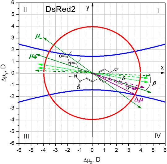
FIGURE 7. Graphical solution of Eq. 16 (blue curves) and Eq. 21 (red curve), to find the Δμ_x and Δμ_y components of Δμ for DsRed2. The structure of the DsRed2 chromophore is displayed in the background, illustrating the molecular system of coordinates. Green dashed bi-directional arrows depict the direction of the oscillating transition dipole moment μ, calculated in (List et al., 2012), for the chromophore in vacuum (light green) and in DsRed protein (dark green). The dotted light green arrow corresponds to a direction of μ calculated in vacuum in (Ansbacher et al. 2012). Purple dashed arrows correspond to the quantum mechanically calculated Δμ vector in DsRed protein environment described by three different models (List et al., 2012); see text. The purple solid arrow is the selected Δμ solution of Eqs 16,21. It was selected based on the known Δμ and μ vectors calculated in (List et al., 2012) and our MD simulations of the electric field; see text. Green solid bi-directional arrows represent the two possible directions of the μ vector based on our measurement of γ and the selected direction of Δμ.

Knowing the direction of Δμ in a protein and angle γ, we can predict the direction of μ from our own experiments. Since Ω measures only an absolute value of γ, there will be two possible directions of μ for each pair of quadrants: I-III and II-IV. Suppose that Δμ lies within either quadrants II or IV, then two solutions for μ, μ₊ and μ₋ would be possible (Figure 7). The direction of μ₊ agrees better with the calculations of (List et al., 2012; Ansbacher, et al., 2012). Solutions corresponding to quadrants I and III result in worse agreement with theoretically predicted β. Therefore, all the evidence presented above suggests that the Δμ vector most probably falls within quadrant IV, as shown in Figure 7. Its numerical components (Δμ_x and Δμ_y) are presented in Table 3. Note that the direction of Δμ corresponds to a flow of electronic density globally from P to I and further to A.

TABLE 3

Table 3. Components of Δμ vector and corresponding electric fields for a series of RFPs.

The dipole vector diagrams for other proteins (similar to Figure 7) are shown in Supplementary Figure S1. It is interesting to note that the direction of μ in mCherry (β = −8.70°) was recently measured independently in crystal (Myskova et al., 2020) and it is very close to what was predicted theoretically for the isolated chromophore (β = -(6÷10°) (List et al., 2012; Ansbacher, et al., 2012) and for the DsRed protein (β = −(3–6)°) (List et al., 2012). The β angles obtained in liquid solution with our model for μ₊ (β = −19° for DsRed2 and −28° for mCherry pH 7.4) are close, but systematically larger in absolute value than those either calculated or measured in crystals. We think that this discrepancy is because the chromophore can visit a larger set of conformations in solution, allowing the acylimine tail to come into better conjugation with the rest of the molecule, thus turning μ closer to the direction of the tail. Note that the direction of the μ vector is quite conservative for the whole set of proteins studied here, with values between −19° to −35° (Table 2 and Supplementary Figure S1).

Our next step is to calculate the E_x and E_y components of the electric field from the experimentally defined Δμ_x and Δμ_y, using Eqs 12, 13. The results, that we call “quasi-empirical”, are presented in Table 3 and Supplementary Table S1. To validate our “quasi-empirical” electric fields and to obtain an additional support for the direction of Δμ vector not only in DsRed but in other RFPs, we performed a series of MD simulations on DsRed, mCherry pH 7.4, mCherry pH 11.4, and mPlum. In this case, electric fields were obtained as negative derivatives of the time-averaged potentials on chromophore atoms along the π-conjugation pathway and projected onto the x- or y-direction, as was done before for GFPs (Drobizhev et al., 2015). We used the chains of atoms: CD2-CG2-CB2-CA2-C2 for E_x and O2-C2-CA2 for E_y evaluations (see Figure 4 for atoms labeling). The results of these calculations are presented in Supplementary Figure S2 and Supplementary Table S1. Although in some cases the agreement between the experimental and calculated values of the fields is almost quantitative, i.e., within the standard deviations (mCherry pH 7.4 and pH 11.4, if Δμ is in quadrant IV), in others they agree qualitatively (DsRed and mPlum). Considering the direction of Δμ in DsRed and mCherry (at pH 7.4 and 11.4), the best match between our “quasi-empirical” model and MD simulations is obtained for Δμ falling in quadrant IV. For mPlum, the best match corresponds to quadrant III, with quadrant IV being the next closest. If Δμ of mPlum in fact would lie in quadrant III, the μ vector would adopt a quite unexpected direction, through quadrants I and III. We consider this improbable because of the “conservation” law for the direction of μ, see (List et al., 2012; Ansbacher, et al., 2012), Table 2, and Supplementary Figure S1. Therefore, we assume that Δμ of mPlum is within quadrant IV, like in the other three proteins. The components of the Δμ vector and electric field in all the proteins and in different conformational states, are summarized in Table 3.

Describing the Rate of TICT Process With Marcus Formalism

We now consider another possible mechanism of fluorescence quenching–ultrafast nonradiative transition (jump) from the excited to the ground state, when the RFP chromophore adopts a twisted conformation at a conical intersection seam. Prior to this event, the chromophore in the excited state proceeds through a slower process of twisting of its phenolate group around the bridging CG2-CB2 bond (Olsen and Smith, 2007; Sun et al, 2012; Moron et al., 2019). According to calculations, the twisting occurs in concert with significant CT across the bridge from the P to the I and A groups. When the angle between P and I rings becomes ∼75°–90°, a whole electronic density of the excited state orbital localizes on the I and A parts (Olsen and Smith, 2007). The charge q = 0.32e (e is the electron charge) is transferred from P to A and I in the TICT process (Olsen and Smith, 2007).

TICT is common for many molecules featuring electron-donating and accepting groups capable of rotating relative to each other around a bridging bond (Grabowski et al., 2003). If the final CT state is stabilized by a polar solvent, the fluorescence quantum yield drops dramatically (Grabowski et al., 2003), pointing to the dependence of the CT rate on the thermodynamic free energy difference. We hypothesize that in RFPs, the protein electric field can contribute to stabilization (or destabilization) of the TICT state in RFPs. If, for example, the field directed from I to P (E_x) increases (corresponding to concentration of more positive charges on the imidazolinone site and/or more negative charges on the phenyl side in a certain mutant), the CT is expected to accelerate and the conical intersection seam will be reached faster.

In our model, we assume that the potential energy barrier for rotation from a planar to a strongly twisted chromophore is due to steric interactions of the P ring with nearby residues above and below the ring plane. In the RFPs studied here, the most important residues in these positions making direct van der Waals contacts with P are Pro63 (substituted to Thr in eqFP670), Met163 (Lys in DsRed2), and Ile197 (Ala in DsRed2, Arg in mScarlet and eqFP670), as well as Lys70 in DsRed2; see Supplementary Table S3. For our model we assume a priori that the barrier is equal for all proteins, i.e., two parabolic potentials corresponding to the initial and final states in the Marcus model always have same stiffness. The electric field, however, changes between proteins, as we have seen.

To correlate the barrier height with a change of free energy, we use Marcus theory formalism. We assume that the rate of TICT in the excited state is a limiting stage for nonradiative relaxation. Therefore, according to the Marcus theory in the high temperature limit, we can write (Sutin, 1999; Bixon and Jortner, 1999):

$k_{nR }=B{e}^{-\frac{{(\Delta G^0+\lambda )}^2}{4\lambda k_{B}T}},(28)$

where ΔG° is the standard Gibbs free energy change in the CT reaction, λ is the reorganization energy, k_B is the Boltzmann factor, and T is the absolute temperature. The high temperature limit (hν_V < k_BT, where ν_V is the frequency of vibration coupled with CT) can be justified for different low-frequency modes, such as collective vibrations of protein beta-barrel, ν_V = (1.5–9) × 10¹¹ s⁻¹, (Martin and Matyushov, 2012; Hu et al., 2012; Perticaroli et al., 2014), or twisting modes of the chromophore itself, (3–6) × 10¹² s⁻¹ (Martin et al., 2004). The pre-exponential factor B for a single low-frequency mode ν_V can be presented as B = κν_V, where κ is the Landau–Zener dimensionless transmission coefficient (Bixon and Jortner, 1999). If κ << 1, the process is considered non-adiabatic, and if κ = 1, it is adiabatic. In the non-adiabatic limit,

$B=\left(\frac{4{\pi }^2}{h}\right)V^2{\left(4\pi k_{B}T\lambda \right)}^{-1/2},(29)$

where V is the electronic coupling parameter. Note that Eqs 28, 29 can be derived independently (of Marcus theory) on the basis of the more general Fermi golden rule for nonradiative electron-vibrational transitions when only low-frequency modes are involved (Bixon and Jortner, 1999; Callis and Liu, 2004).

Taking the logarithm of both sides in Eq. 28, we obtain

$\ln \left(k_{nR }\right)=\ln B-\frac{{\left(\Delta G^0+\lambda \right)}^2}{4\lambda k_{B}T}.(30)$

Suppose that a negative point charge of an absolute value q is transferred by a distance Δx opposite to the x-axis direction and a distance Δy opposite to the y-axis direction, see Figure 4 for definition of x and y directions. For simplicity, we consider a point charge moving from the geometric center of the initial charge distribution on P (corresponding to a locally excited state) to the geometrical center of the final charge distribution on I and A (corresponding to a TICT state). We assume that the parameters q, Δx, and Δy are the same for all the proteins. If an electric field E = (E_x, E_y) is present in course of the charge transfer, the electrostatic potential energy of the system will change by

$\Delta U=-q\Delta x{E}_x-q\Delta y{E}_y=-q\Delta x\left(E_x+\eta E_y\right), \text{where }\eta =\Delta y/\Delta x.(31)$

We assume that the field does not change during the process of charge transfer and is the same as that found in previous section. The total free energy change, ΔG⁰, consists of a pure molecular (vacuum) part, ΔG⁰_vac, and an electrostatic part (imposed by the protein) ΔU:

$\text{Δ}{G}^0=\text{Δ}{G}_{vac}^0-q\text{Δ}x\left(E_x+\eta E_y\right).(32)$

Substituting this into Eq. 30, we obtain

$\ln k_{nR }=b_0+b_1\left(E_x+\eta E_y\right)+b_2{\left(E_x+\eta E_y\right)}^2,(33)$

which is a second-order polynomial in terms of $E_x+\eta E_y$. In Eq 33, the constant parameters are defined as follows:

$b_0=\ln B-\frac{\lambda }{4k_{B}T}-\frac{\Delta G_{vac}^0}{2k_{B}T}-\frac{{\left(\Delta G_{vac}^0\right)}^2}{4\lambda k_{B}T},(34)$

$b_1= \frac{q\Delta x}{2k_{B}T}\left[1+\frac{\Delta G_{vac}^0}{\lambda }\right],(35)$

$b_2=-\frac{{\left(q\Delta x\right)}^2}{4\lambda k_{B}T}(36)$

Using our experimental results, we plotted lnk_nR vs. $\left(E_x+\eta E_y\right)$, varying the parameter η from −0.2 to 0.1 (Supplementary Figure S3). Out of seven proteins, five (DsRed2, mCherry pH 7.4, mCherry pH 11.4, and red-shifted forms of XRFP and mPlum) fit satisfactorily to a second order polynomial in this range of η. mScarlet and eqFP670 drop significantly out of the correlation and therefore we do not include them in the fit (see discussion below). For each η value, the residual sum of squares of the fit was calculated and the minimum was achieved at η = −0.1 (Supplementary Figure S4). The final plot of  lnk_nR vs $\left(E_x+\eta E_y\right)$ corresponding to η = −0.1 is shown in Figure 8.

FIGURE 8

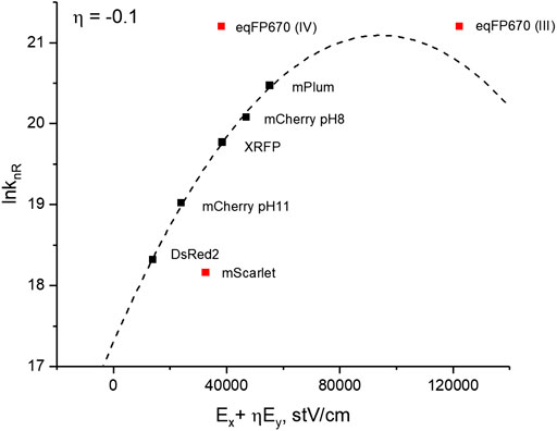
FIGURE 8. Dependence of nonradiative decay rate (in logarithmic scale) on the change of electrostatic potential energy normalized to the product of charge displacement along x-direction (Δx) and the value of charge (q). Theoretical fit of the model function Eq. 33 to the data obtained for five proteins (black symbols) is shown by dashed line. mScarlet and eqFP670 data points (red squares) are not included in the fit (see text). Red square labeled eqFP670 (IV) correspond to the electric field calculated from the Δμ position in quadrant IV, and eqFP670 (III)—to Δμ position in quadrant III.

In their consideration of TICT, Olsen and Smith calculated the parameters G⁰_vac and q for the isolated RFP chromophore; see Figure 7 of (Olsen and Smith, 2007). We use these values as well as three experimental coefficients, b₀, b₁, and b₂, corresponding to the best fit of our data to the Marcus model (Figure 8) to find the final three parameters: λ, Δx, and B from the system of Eqs 34–36. The transversal displacement Δy was then calculated according to Δy = η Δx. All the parameters are reported in Table 4. (Other Δx and Δy values calculated from the best fits for different η values are presented in Supplementary Table S2) Note that the found B factor (Table 4) is much smaller than the vibrational frequencies ν_V mentioned above. This suggests non-adiabatic character of CT (κ << 1) and justifies applicability of Eq 28. It is interesting that the obtained charge displacement Δx = 6.7 Å is close to the actual chromophore size and to the displacements predicted theoretically in (Olsen and Smith, 2007; Moron et al., 2019). The positive sign of Δx supports the prediction that the electronic density is moving from P to I, and the negative sign and magnitude of Δy (−0.67 Å) suggests a further slight shift from I to A, in qualitative agreement with predictions (Olsen and Smith, 2007).

TABLE 4

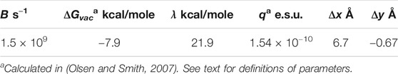
TABLE 4. TICT parameters of the RFP chromophore.

To estimate more accurately the theoretically predicted magnitude of charge displacement (Olsen and Smith, 2007), we first notice that a part of the LUMO density, localized on the phenolate group before the transfer, is centered close to the middle point between the CE1 and CE2 atoms (Gross et al., 2000; Mochizuki et al., 2007; Hasegawa et al., 2010; List et al., 2012). Furthermore, the electronic density in a 90⁰ P-twisted conformation is delocalized between I and A groups (Olsen and Smith, 2007), with a much higher weight on I than on A (Moron et al., 2019). Therefore, we can assume that the charge density moves from the point between the CE1 and CE2 atoms (whose position does not move during the P rotation) to the C1 atom of imidazolinone. The corresponding crystallographic values (see, e.g., 2H5Q pdb structure for mCherry) in this case are Δx = 6.1 Å and Δy = −0.9 Å, both in good agreement with our findings (Table 4). These results provide strong independent support both for our approach of finding protein electric fields and for describing the field effect in the framework of TICT. Although five proteins of the series fit quite well to the theoretical model, mScarlet and eqFP670 show significant discrepancies.

Special Case: mScarlet

In the case of mScarlet, the experimental nonradiative rate is much slower than what is expected from the values of the field. This can be explained by the very tight surrounding of the chromophore that strongly elevates the steric energy barrier for P rotation (Bindels et al., 2017). More specifically, instead of the flexible, neutral Ile197 in mFruits, mScarlet has an Arg residue that faces the phenolate ring and makes multiple van der Waals contacts with it, impeding the P-rotation. Moreover, the Arg side group in mScarlet makes a cobweb of numerous hydrogen bonds that holds it more strongly in place compared to Ile in mFruits and Ala in DsRed2. In the original publication (Bindels et al, 2017), these strong local interactions were invoked to explain the exceptionally planar structure of mScarlet chromophore observed in crystal.

Special Case: eqFP670

In the case of eqFP670, the fluorescing state most probably corresponds to a different conformation of the chromophore/environment in the excited state compared to the ground state, see Section “Finding Dipole Moment Difference Δμ and the Angle γ between the Vectors μ and Δμ”. Unfortunately, this conformation cannot be interrogated with 2PA (in contrast to mPlum and XRFP), because it is not present in the ground state. Therefore, we can only speculate about the values of the electric field corresponding to this conformer. Suppose that Δμ and the field in the excited state are not very different from the ground state, and that the Δμ vector lies in quadrant IV (Supplementary Figure S1). Then the nonradiative rate turns out to be several times too fast compared to the expected value based on the model fit (left red square in Figure 8).

However, one cannot rule out the possibility that the Δμ of eqFP670 occupies another quadrant. For instance, the direction of Δμ_x can flip if E_x reaches some critical value. This flipping can theoretically occur at $E_x^{\ast }=-\text{Δ}{\mu }_{0,x}/\text{Δ}{\alpha }_{xx}=27\text{ MV}/\text{cm}$; see Eq. 10. The k_nR value steadily increases in concert with E_x in the series of DsRed2, mCherry pH 11.4, XRFP, mCherry pH 7.4, and mPlum (Table 3). Therefore, one would expect an even larger E_x value for eqFP670 than for mPlum (i.e., >19 MV/cm), instead of the predicted E_x = 14 MV/cm (if Δμ is in quadrant IV). If this were true, it could lead to a negative Δμ_x. This situation would correspond to a position of Δμ in quadrants II or III with E_x = 39.5 MV/cm for both cases. Choosing between quadrants II and III depends on the direction of Δμ_y. If Δμ_y > 0, i.e., Δμ is flipped relatively to its direction in IV and lies in quadrant II, then the predicted E_y value becomes very large (∼250 MV/cm) compared to the rest of the proteins (30–60 MV/cm). This is difficult to explain considering that the electrostatic environment in eqFP670 is not so different from the others. (Estimations show that an additional positive Arg197 and a conserved, presumably negative Glu215, can explain some increase in E_y value of eqFP670 versus mFruits, but not larger than up to a factor of 2.) Therefore, we assume that a position of Δμ in quadrant III is possible, and we show a data point for eqFP670 corresponding to this quadrant in Figure 8 (right red square). This point is reasonably close to the model fit and provides E_x = 39.5 MV/cm and E_y = 28.3 MV/cm.

Mechanistically, a large value of E_x in eqFP670 (relative to other RFPs) can tentatively be explained by the presence of the Asn143 residue close to the phenolate oxygen of the chromophore. As the crystal structure (4EDS pdb) shows, the carbonyl oxygen atom OD1 of the Asn143 side chain comes in unusually close contact to the phenolate oxygen (∼2.4 Å), which is shorter than the sum of their van der Waals radii. A hydrogen bonding network built around the chromophore phenolate and the Asn143 residue probably helps to hold the two electronegative atoms in such a close contact. Since the Asn carbonyl oxygen carries a partial negative charge, this can result in pushing the negative charge of the phenolate oxygen toward other parts of the chromophore (e.g., I or A). This effect is analogous to an increase of the effective electric field in the x-direction that potentially flips the sign of Δμ_x.

Discussion

It was suggested on theoretical grounds that the nonradiative relaxation of the red FP chromophore in vacuum (Olsen and Smith, 2007) or in proteins (Sun et al., 2012; Moron et al., 2019) generally proceeds via TICT with the phenolate ring turning from 0° to ∼75°–90° around the adjacent C–C bridging bond. This process leads to a conical intersection of the S₁ and S₀ potential energy surfaces that opens a doorway for almost instantaneous S₁ ∼> S₀ relaxation. The phenolate rotation is barrierless for chromophore in vacuum, but encounters a potential barrier in proteins due to steric interactions between the phenolate ring and few nearby amino acid side chains. Since the twisting is coupled to significant charge transfer in the excited state, an external (to the chromophore) electric field could either facilitate or hinder this process, depending on its strength and direction. We apply the Marcus formalism to correlate the barrier height and the free energy difference (ΔG⁰) between the final and initial states of the charge transfer. In this model, the ΔG⁰ contains a contribution equal to the change of electrostatic potential energy between the two states. We observe that for five out of seven proteins, including DsRed2, mCherry (pH 7.4 and pH 11.4), mPlum, and XRFP, the radiationless relaxation rate follows the Marcus theory.

For mScarlet, the measured nonradiative rate is much slower than predicted by the model. We explain this by a much higher potential barrier for rotation of phenolate because of steric clashes with the R198 and Pro64 side chains. The former occupies a unique position on top of the phenolate group and makes several van der Waals contacts with it. The second flanks the phenolate from the opposite side and due to its rigid nature provides an additional barrier for P-rotation. Therefore, we can conclude that a combination of these two amino acids in the chromophore pocket is probably a main factor securing high brightness of mScarlet, compared to, e.g., XRFP (experiencing similar electric field, Figure 8).

In contrast, the nonradiative rate of eqFP670 appears to be larger than predicted by our model, for both possible directions of Δμ, i.e. in quadrants III and IV, Figure 8. Although field-facilitated TICT can qualitatively explain the very fast nonradiative rate of eqFP670 (see previous section), other mechanisms cannot be ruled out. One is vibrational relaxation, described by the energy gap law (“Checking the Energy Gap Law” section). For a far-red emitting protein such as eqFP670, this mechanism can strongly contribute to an increase of k_nR. Another possibility is that some other molecular parameters involved in TICT are different in eqFP670 compared to other RFPs. These include the charge q, and CT distances Δx or Δy, as well as the potential barrier to rotation. Differences in any of the first three are probable, especially if the acylimine tail adopts a different conformation during the process of excited state relaxation similar to what was suggested in mPlum (Moron et al., 2019). There are two different factors that could affect the height of potential barrier for P-rotation. First, similar to mScarlet, the phenolate of eqFP670 is flanked by Arg197 with four van der Waals contacts between them (although in mScarlet there are six). Also, Arg197 participates in a number of hydrogen bonds that hold its position fixed. On the other hand, the more flexible Thr60 found on the opposite side of the phenolate group in eqFP670, replacing the rigid cycle of the Pro63 residue, probably makes phenolate rotation easier.

If we only consider the RFPs with a “moderately-soft” internal pocket around phenolate group, i.e., similar to those containing Pro63 and Ile197 (or Ala197), we can establish some qualitative structure-property relationships for photophysical parameters that can potentially help to guide future RFP engineering. Figure 9A shows a 3D plot of the quantum yield as a function of the electric field components E_x and E_y. The quantum yield is calculated using Eq. 2 with k_R = 0.158 × 10⁹ s⁻¹ (mean of all seven k_R values, Table 1), and k_nR described by Eqs 33–36. As one can see, for each fixed E_y value, the quantum yield first decreases as E_x increases, then reaches a minimum, and then starts to increase. For all reasonable E_y values, in the region of negative E_x values, the potential barrier for TICT via P-rotation becomes very high due to the combined action of the “charge locking” effect of E_x and steric clashes of phenolate with nearby residues. This results in φ = 1.

FIGURE 9

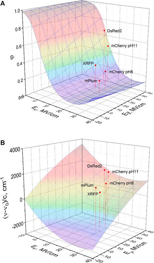
FIGURE 9. 3D plot representing quantum yield (A) and shift of peak absorption transition frequency relative to the vacuum frequency (B) as a function of E_x and E_y in a set of RFPs with a “moderately-soft” phenolate pocket (see text). Five representative RFPs are shown by red dots. Large quantum yields in (A) correspond to red and small quantum yields—to purple color of the surface. The calculation is based on model Eqs 2, 33–36 and model parameters presented in Table 4. Large negative shifts in (B) corresponds to purple and large positive shifts—to red surface color. The prediction is based on Eq. 15 and parameters from “Parameters of the Isolated RFP Chromophore Calculated Quantum Mechanically” section.

With increasing positive E_x, the barrier becomes lower, thus accelerating nonradiative relaxation. The k_nR reaches its maximum (minimum φ) when ΔG⁰ = −λ, in accord with the Marcus model. Even larger E_x values correspond to a so-called inverted Marcus region (Bixon and Jortner, 1999), where the k_nR rate starts to decrease again and quantum yield to increase. For a fixed E_x within the normal Marcus region, φ increases with the increase of E_y, but the absolute values of gradients are much smaller than for E_x. This behavior follows from the fact that the charge is transferred counter to the E_y field, but at a much shorter distance compared to the x-direction. For an illustration, we show the data points corresponding to DsRed2, mCherry pH 11.4, mCherry pH 7.4, mPlum, and XRFP. The transition from DsRed2 to mCherry pH 11.4 corresponds to the drop of quantum yield by 30%, following an increase of E_x by 3 MV/cm (with E_y unchanged), whereas transition from mCherry pH 7.4 to mPlum also corresponds to a drop of φ by 30%, but with the decrease of E_y by 12 MV/cm (with almost constant E_x value).

The absorption frequency shift (relatively to vacuum ${\overline{\nu }}_0$ = 16,260 cm⁻¹, λ_abs,0 = 615 nm) as a function of E_x and E_y is presented in Figure 9B. It is calculated according to Eq. 14. Here, the further red-shifted variants correspond to small positive (or, better, even negative) E_y values simultaneously with E_x values around 20–30 MV/cm. To have both a red-shifted absorption and a reasonably high quantum yield, one has to keep both E_x and E_y in the range of small positive or negative values, i.e., from −10 to +10 MV/cm. A favorably low E_x of the DsRed2 protein leading to a high quantum yield is most likely due to the positively charged Lys163 residue hydrogen-bonded to the phenolate oxygen. In mFruits and mScarlet, E_x is larger, probably because of lacking of the charge in that position.

Possible mutagenesis strategy for optimizing both parameters (φ and λ_abs) using the DsRed scaffold could contain the following steps. First, one should keep a positively charged residue H-bonded to the phenolate oxygen (to have a small E_x). Second, one should concentrate more positive charges close to the acylimine oxygen (to decrease E_y) and/or more negative charge on the imidazolinone carbonyl oxygen (to further decrease E_x and decrease E_y). The last change may be a difficult task however, because the Arg95 residue hydrogen bonding to the imidazolinone oxygen seems to be conservative in RFPs. It is interesting that similar recipes for improving quantum yield and shifting fluorescence to the red were put forward on the basis of quantum calculations of several different mPlum conformers (Moron et al., 2019).

We finally would like to note that in the case of two-photon excitation, peak absorption wavelengths of RFPs automatically fall in the tissue transparency window and therefore the 2P brightness, but not the position of 2PA peak becomes a most critical parameter. The relative 2P brightness can be estimated to a first approximation as a product Δμ²φ. Both Δμ² and φ depend on the electric field and our model, see Figure 10, predicts that for getting 2P brighter variants one has to decrease or even flip the sign of E_x component, with E_y playing not too critical role. The structural guidelines for increasing 2P brightness are therefore similar to what was described above for obtaining higher quantum yield.

FIGURE 10

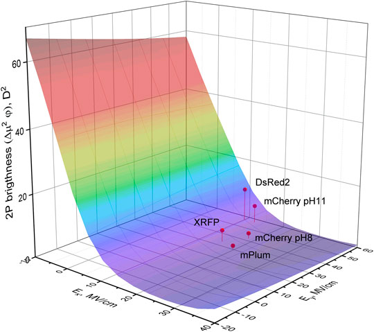
FIGURE 10. 3D plot representing the 2P brightness (roughly proportional to Δμ²φ) in the region of the 0–0 excitation frequency as a function of E_x and E_y. Large brightness corresponds to red color on the surface and small brightness—to purple. Four representative RFPs are shown by red dots.

Data Availability Statement

The original contributions presented in the study are included in the article/Supplementary Material, further inquiries can be directed to the corresponding author.

Author Contributions

MD and TH conceived the idea of the paper and supervised the project, MD and RM wrote the paper, MD and RM made experimental measurements, RM expressed and purified all the proteins, MD developed the physical models, PC and JS accomplished quantum mechanical and molecular dynamics simulations, GL, AS, and NS engineered XP fluorescent protein.

Funding

This work was supported by the NINDS grants U01 NS094246 (MD, TH, and RM), U24 NS109107 (MD, TH, and RM), U01 NS099709 (NS), U01NS113294 (NS), the Ruth L. Kirschstein National Research Service Award, number F31NS108593 (RM), NIGMS grants R01 GM109984 (NS) and R01 GM121944 (NS), NEI grant R21EY030716 (NS), and NSF grant NeuroNex 1707352 (NS).

Conflict of Interest

JNS is the owner of the company JNScott Consulting, LLC.

The remaining authors declare that the research was conducted in the absence of any commercial or financial relationships that could be construed as a potential conflict of interest.

Acknowledgments

We thank Josef Lazar for fruitful discussion and for sharing unpublished data and Merrilee Thomas for technical help with expression and purification of mScarlet. Computational support was provided by Extreme Science and Engineering Discovery Environment (XSEDE) allocations to PC (TG-MCB090176).

Supplementary Material

The Supplementary Material for this article can be found online at: https://www.frontiersin.org/articles/10.3389/fmolb.2021.633217/full#supplementary-material.

References

Abbyad, P., Childs, W., Shi, X., and Boxer, S. G. (2007). Dynamic Stokes shift in green fluorescent protein variants. Proc. Natl. Acad. Sci. U.S.A. 104 (51), 20189–20194. doi:10.1073/pnas.0706185104

PubMed Abstract | CrossRef Full Text | Google Scholar

Afgan, E., Baker, D., Batut, B., van den Beek, M., Bouvier, D., Cech, M., et al. (2018). The Galaxy platform for accessible, reproducible and collaborative biomedical analyses: 2018 update. Nucleic Acids Res. 46, W537–W544. doi:10.1093/nar/gky379

PubMed Abstract | CrossRef Full Text | Google Scholar

Altoe, P., Bernardi, F., Garavelli, M., Orlandi, G., and Negri, F. (2005). Solvent effects on the vibrational activity and photodynamics of the green fluorescent protein chromophore: a quantum-chemical study. J. Am. Chem. Soc. 127 (11), 3952–3963. doi:10.1021/ja0451517

PubMed Abstract | CrossRef Full Text | Google Scholar

Ansbacher, T., Srivastava, H. K., Stein, T., Baer, R., Merkx, M., and Shurki, A. (2012). Calculation of transition dipole moment in fluorescent proteins–towards efficient energy transfer. Phys. Chem. Chem. Phys. 14 (12), 4109–4117. doi:10.1039/c2cp23351g

PubMed Abstract | CrossRef Full Text | Google Scholar

Atkins, P. W., and Friedman, R. S. (1997). Molecular Quantum Mechanics. Oxford, New York, Tokyo: Oxford University Press.

Google Scholar

Berlin, Y., Burin, A., Friedrich, J., and Köhler, J. (2006). Spectroscopy of proteins at low temperature. Part I: Experiments with molecular ensembles. Phys. Life Rev. 3 (4), 262–292. doi:10.1016/j.plrev.2006.09.001

CrossRef Full Text | Google Scholar

Bindels, D. S., Haarbosch, L., van Weeren, L., Postma, M., Wiese, K. E., Mastop, M., et al. (2017). mScarlet: a bright monomeric red fluorescent protein for cellular imaging. Nat. Methods 14 (1), 53–56. doi:10.1038/nmeth.4074

PubMed Abstract | CrossRef Full Text | Google Scholar

Bixon, M., and Jortner, J. (1999). “Electron transfer - from isolated molecules to biomolecules,” in Electron Transfer–From Isolated Molecules to Biomolecules. Pt. 1. Editor J. Jortner, and M. Bixon (New York: Wiley), 35–203.

Google Scholar

Bloebmergen, N. (1965). Nonlinear Optics. New York: Benjamin.

Google Scholar

Boens, N., Qin, W., Basarić, N., Hofkens, J., Ameloot, M., Pouget, J., et al. (2007). Fluorescence lifetime standards for time and frequency domain fluorescence spectroscopy. Anal. Chem. 79 (5), 2137–2149. doi:10.1021/ac062160k

PubMed Abstract | CrossRef Full Text | Google Scholar

Callis, P. R., and Burgess, B. K. (1997). Tryptophan fluorescence shifts in proteins from hybrid simulations: an electrostatic approach. J. Phys. Chem. B 101 (46), 9429–9432. doi:10.1021/jp972436f

CrossRef Full Text | Google Scholar

Callis, P. R., and Liu, T. (2004). Quantitative prediction of fluorescence quantum yields for tryptophan in proteins. J. Phys. Chem. B 108 (14), 4248–4259. doi:10.1021/jp0310551

CrossRef Full Text | Google Scholar

Chudakov, D. M., Feofanov, A. V., Mudrik, N. N., Lukyanov, S., and Lukyanov, K. A. (2003). Chromophore environment provides clue to “kindling fluorescent protein” riddle. J. Biol. Chem. 278 (9), 7215–7219. doi:10.1074/jbc.M211988200

PubMed Abstract | CrossRef Full Text | Google Scholar

Chudakov, D. M., Matz, M. V., Lukyanov, S., and Lukyanov, K. A. (2010). Fluorescent proteins and their applications in imaging living cells and tissues. Physiol. Rev. 90 (3), 1103–1163. doi:10.1152/physrev.00038.2009

PubMed Abstract | CrossRef Full Text | Google Scholar

Cramer, L. E., and Spears, K. G. (1978). Hydrogen bond strengths from solvent-dependent lifetimes of Rose Bengal dye. J. Am. Chem. Soc. 100 (1), 221–227. doi:10.1021/ja00469a039

CrossRef Full Text | Google Scholar

Day, R. N., and Davidson, M. W. (2009). The fluorescent protein palette: tools for cellular imaging. Chem. Soc. Rev. 38 (10), 2887–2921. doi:10.1039/b901966a

PubMed Abstract | CrossRef Full Text | Google Scholar

Dmitrienko, D. V., Vrzheshch, E. P., Drutsa, V. L., and Vrzheshch, P. V. (2006). Red fluorescent protein DsRed: Parametrization of its chromophore as an amino acid residue for computer modeling in the OPLS-AA force field. Biochem. Mosc. 71 (10), 1133–1152. doi:10.1134/s0006297906100129

CrossRef Full Text | Google Scholar

Drobizhev, M., Tillo, S., Makarov, N. S., Hughes, T. E., and Rebane, A. (2009). Color hues in red fluorescent proteins are due to internal quadratic Stark effect. J. Phys. Chem. B 113 (39), 12860–12864. doi:10.1021/jp907085p

PubMed Abstract | CrossRef Full Text | Google Scholar

Drobizhev, M., Makarov, N. S., Tillo, S. E., Hughes, T. E., and Rebane, A. (2011). Two-photon absorption properties of fluorescent proteins. Nat. Methods 8 (5), 393–399. doi:10.1038/nmeth.1596

PubMed Abstract | CrossRef Full Text | Google Scholar

Drobizhev, M., Scott, J. N., Callis, P. R., and Rebane, A. (2012a). All-optical sensing of the components of the internal local electric field in proteins. IEEE Photon. J. 4 (5), 1996–2001. doi:10.1109/JPHOT.2012.2221124

CrossRef Full Text | Google Scholar

Drobizhev, M., Makarov, N. S., Tillo, S. E., Hughes, T. E., and Rebane, A. (2012b). Describing two-photon absorptivity of fluorescent proteins with a new vibronic coupling mechanism. J. Phys. Chem. B 116 (5), 1736–1744. doi:10.1021/jp211020k

PubMed Abstract | CrossRef Full Text | Google Scholar

Drobizhev, M., Callis, P. R., Nifosì, R., Wicks, G., Stoltzfus, C., Barnett, L., et al. (2015). Long- and short-range electrostatic fields in GFP mutants: implications for spectral tuning. Sci. Rep. 5, 13223. doi:10.1038/srep13223

PubMed Abstract | CrossRef Full Text | Google Scholar

Drobizhev, M., Molina, R. S., and Hughes, T. E. (2020). Characterizing the two-photon absorption properties of fluorescent molecules in the 680–1,300 nm spectral range. Bio. Protoc. 10 (2), 33. doi:10.21769/BioProtoc.3498

CrossRef Full Text | Google Scholar

Englman, R., and Jortner, J. (1970). The energy gap law for radiationless transitions in large molecules. Mol. Phys. 18 (2), 145–164. doi:10.1080/00268977000100171

CrossRef Full Text | Google Scholar

Faraji, S., and Krylov, A. I. (2015). On the nature of an extended stokes shift in the mplum fluorescent protein. J. Phys. Chem. B 119 (41), 13052–13062. doi:10.1021/acs.jpcb.5b07724

PubMed Abstract | CrossRef Full Text | Google Scholar

Fleming, G. R., Knight, A. W. E., Morris, J. M., Morrison, R. J. S., and Robinson, G. W. (1977). Picosecond fluorescence studies of xanthene dyes. J. Am. Chem. Soc. 99 (13), 4306–4311. doi:10.1021/ja00455a017

CrossRef Full Text | Google Scholar

Fried, S. D., Wang, L. P., Boxer, S. G., Ren, P., and Pande, V. S. (2013). Calculations of the electric fields in liquid solutions. J. Phys. Chem. B 117 (50), 16236–16248. doi:10.1021/jp410720y

PubMed Abstract | CrossRef Full Text | Google Scholar

Frisch, M. J., Trucks, G. W., Schlegel, H. B., Scuseria, G. E., Robb, M. A., Cheeseman, J. R., et al. (2016). Gaussian 09, Revision A.02. Wallingford CT: Gaussian, Inc.

Google Scholar

Geissinger, P., Kohler, B. E., and Woehl, J. C. (1995). Electric field and structure in the myoglobin heme pocket. J. Phys. Chem. 99 (45), 16527–16529. doi:10.1021/j100045a008

CrossRef Full Text | Google Scholar

Gibson, DG, Young, L, Chuang, RY, Venter, JC, Hutchison, CA, and Smith, HO (2009). Enzymatic assembly of DNA molecules up to several hundred kilobases. Nat. Methods 6, 343–345. doi:10.1038/nmeth.1318

PubMed Abstract | CrossRef Full Text | Google Scholar

Grabherr, M. G., Haas, B. J., Yassour, M., Levin, J. Z., Thompson, D. A., Amit, I., et al. (2011). Full-length transcriptome assembly from RNA-Seq data without a reference genome. Nat. Biotechnol. 29, 644–652. doi:10.1038/nbt.1883

PubMed Abstract | CrossRef Full Text | Google Scholar

Grabowski, Z. R., Rotkiewicz, K., and Rettig, W. (2003). Structural changes accompanying intramolecular electron transfer: focus on twisted intramolecular charge–transfer states and structures. Chem. Rev. 103 (10), 3899–4032. doi:10.1021/cr940745l

PubMed Abstract | CrossRef Full Text | Google Scholar

Gross, L. A., Baird, G. S., Hoffman, R. C., Baldridge, K. K., and Tsien, R. Y. (2000). The structure of the chromophore within DsRed, a red fluorescent protein from coral. Proc. Natl. Acad. Sci. U.S.A. 97 (22), 11990–11995. doi:10.1073/pnas.97.22.11990

PubMed Abstract | CrossRef Full Text | Google Scholar

Haas, B. J., Papanicolaou, A., Yassour, M., Grabherr, M., Blood, P. D., Bowden, J., et al. (2013). De novo transcript sequence reconstruction from RNA-seq using the Trinity platform for reference generation and analysis. Nat. Protoc. 8, 1494–1512. doi:10.1038/nprot.2013.084

PubMed Abstract | CrossRef Full Text | Google Scholar

Hasegawa, J. Y., Ise, T., Fujimoto, K. J., Kikuchi, A., Fukumura, E., Miyawaki, A., et al. (2010). Excited states of fluorescent proteins, mKO and DsRed: chromophore-protein electrostatic interaction behind the color variations. J. Phys. Chem. B 114 (8), 2971–2999. doi:10.1021/jp9099573

PubMed Abstract | CrossRef Full Text | Google Scholar

Hu, G., Michielssens, S., Moors, S. L., and Ceulemans, A. (2012). The harmonic analysis of cylindrically symmetric proteins: a comparison of Dronpa and a DNA sliding clamp. J. Mol. Graph Model 34, 28–37. doi:10.1016/j.jmgm.2011.12.005

PubMed Abstract | CrossRef Full Text | Google Scholar

Jacquemin, D. (2016). Excited-state dipole and quadrupole moments: TD-DFT versus CC2. J. Chem. Theory Comput. 12 (8), 3993–4003. doi:10.1021/acs.jctc.6b00498

PubMed Abstract | CrossRef Full Text | Google Scholar

Jung, G., Wiehler, J., and Zumbusch, A. (2005). The photophysics of green fluorescent protein: influence of the key amino acids at positions 65, 203, and 222. Biophys. J. 88 (3), 1932–1947. doi:10.1529/biophysj.104.044412

PubMed Abstract | CrossRef Full Text | Google Scholar

Jung, G., Brockhinke, A., Gensch, T., Hotzer, B., Schwedler, S., and Koydan Weettil, S. (2012). “Fluorescence lifetime of fluorescent proteins,” in Fluorescent Protein 1. From Understanding to Design. Editor G. Jung (Berlin: Springer), 69–97. Ch. 11

Google Scholar

Konold, P., Regmi, C. K., Chapagain, P. P., Gerstman, B. S., and Jimenez, R. (2014). Hydrogen bond flexibility correlates with Stokes shift in mPlum variants. J. Phys. Chem. B 118 (11), 2940–2948. doi:10.1021/jp412371y

PubMed Abstract | CrossRef Full Text | Google Scholar

Lakowicz, J. R., Laczko, G., and Gryczynski, I. (1986). 2‐GHz frequency‐domain fluorometer. Rev. Sci. Instrum. 57 (10), 2499–2506. doi:10.1063/1.1139215

CrossRef Full Text | Google Scholar

Lakowicz, J. R. (2006). Principles of Fluorescence Spectroscopy. 3rd Ed. Berlin: Springer.

Google Scholar

Li, J., Williams, B., Cramer, C. J., and Truhlar, D. G. (1999). A class IV charge model for molecular excited states. J. Chem. Phys. 110 (2), 724–733. doi:10.1063/1.478180

CrossRef Full Text | Google Scholar

Lin, M. Z., McKeown, M. R., Ng, H. L., Aguilera, T. A., Shaner, N. C., Campbell, R. E., et al. (2009). Autofluorescent proteins with excitation in the optical window for intravital imaging in mammals. Chem. Biol. 16 (11), 1169–1179. doi:10.1016/j.chembiol.2009.10.009

PubMed Abstract | CrossRef Full Text | Google Scholar

List, N. H., Olsen, J. M., Jensen, H. J., Steindal, A. H., and Kongsted, J. (2012). Molecular-level insight into the spectral tuning mechanism of the DsRed chromophore. J. Phys. Chem. Lett. 3 (23), 3513–3521. doi:10.1021/jz3014858

PubMed Abstract | CrossRef Full Text | Google Scholar

Lounis, B., Deich, J., Rosell, F. I., Boxer, S. G., and Moerner, W. E. (2001). Photophysics ofDsRed, a red fluorescent protein, from the ensemble to the single-molecule level. J. Phys. Chem. B 105 (21), 5048–5054. doi:10.1021/jp010116x

CrossRef Full Text | Google Scholar

Magde, D., Wong, R., and Seybold, P. G. (2002). Fluorescence quantum yields and their relation to lifetimes of rhodamine 6G and fluorescein in nine solvents: improved absolute standards for quantum yields. Photochem. Photobiol. 75 (4), 327–334. doi:10.1562/0031-8655(2002)075<0327:fqyatr>2.0.co;2

PubMed Abstract | CrossRef Full Text | Google Scholar

Manas, E. S., Vanderkooi, J. M., and Sharp, K. A. (1999). The effects of protein environment on the low temperature electronic spectroscopy of cytochromecand microperoxidase-11. J. Phys. Chem. B 103 (30), 6334–6348. doi:10.1021/jp9908552

CrossRef Full Text | Google Scholar

Martin, D. R., and Matyushov, D. V. (2012). Non-Gaussian statistics and nanosecond dynamics of electrostatic fluctuations affecting optical transitions in proteins. J. Phys. Chem. B 116 (34), 10294–10300. doi:10.1021/jp305757t

PubMed Abstract | CrossRef Full Text | Google Scholar

Martin, M. E., Negri, F., and Olivucci, M. (2004). Origin, nature, and fate of the fluorescent state of the green fluorescent protein chromophore at the CASPT2//CASSCF resolution. J. Am. Chem. Soc. 126 (17), 5452–5464. doi:10.1021/ja037278m

PubMed Abstract | CrossRef Full Text | Google Scholar

Masters, T. A., Marsh, R. J., Blacker, T. S., Armoogum, D. A., Larijani, B., and Bain, A. J. (2018). Polarized two-photon photoselection in EGFP: Theory and experiment. J. Chem. Phys. 148 (13), 134311. doi:10.1063/1.5011642

PubMed Abstract | CrossRef Full Text | Google Scholar

Matz, M. V., Fradkov, A. F., Labas, Y. A., Savitsky, A. P., Zaraisky, A. G., Markelov, M. L., et al. (1999). Fluorescent proteins from nonbioluminescent Anthozoa species. Nat. Biotechnol. 17 (10), 969–973. doi:10.1038/13657

PubMed Abstract | CrossRef Full Text | Google Scholar

Meath, W. J., and Power, E. A. (1984). On the importance of permanent moments in multiphoton absorption using perturbation theory. J. Phys. B: At. Mol. Phys. 17, 763–781. doi:10.1088/0022-3700/17/5/017

CrossRef Full Text | Google Scholar

Mochizuki, Y., Nakano, T., Amari, S., Ishikawa, T., Tanaka, K., Sakurai, M., et al. (2007). Fragment molecular orbital calculations on red fluorescent protein (DsRed). Chem. Phys. Lett. 433 (4), 360–367. doi:10.1016/j.cplett.2006.11.088

CrossRef Full Text | Google Scholar

Molina, R. S., Tran, T. M., Campbell, R. E., Lambert, G. G., Salih, A., Shaner, N. C., et al. (2017). Blue-Shifted green fluorescent protein homologues are brighter than enhanced green fluorescent protein under two-photon excitation. J. Phys. Chem. Lett. 8 (12), 2548–2554. doi:10.1021/acs.jpclett.7b00960

PubMed Abstract | CrossRef Full Text | Google Scholar

Molina, R. S., Qian, Y., Wu, J., Shen, Y., Campbell, R. E., Drobizhev, M., et al. (2019). Understanding the fluorescence change in red genetically encoded calcium ion indicators. Biophys. J. 116 (10), 1873–1886. doi:10.1016/j.bpj.2019.04.007

PubMed Abstract | CrossRef Full Text | Google Scholar

Moron, V., Marazzi, M., and Wanko, M. (2019). Far red fluorescent proteins: where is the limit of the acylimine chromophore? J. Chem. Theory Comput. 15 (7), 4228–4240. doi:10.1021/acs.jctc.9b00070

PubMed Abstract | CrossRef Full Text | Google Scholar

Myskova, J., Rybakova, O., Brynda, J., Khoroshyy, P., Bondar, A., and Lazar, J. (2020). Directionality of light absorption and emission in representative fluorescent proteins. Proc. Natl. Acad. Sci. 117 (51), 32395–32401.

Google Scholar

Nifosí, R., Amat, P., and Tozzini, V. (2007). Variation of spectral, structural, and vibrational properties within the intrinsically fluorescent proteins family: a density functional study. J. Comput. Chem. 28 (14), 2366–2377. doi:10.1002/jcc.20764

PubMed Abstract | CrossRef Full Text | Google Scholar

Nifosì, R., Mennucci, B., and Filippi, C. (2019). The key to the yellow-to-cyan tuning in the green fluorescent protein family is polarisation. Phys. Chem. Chem. Phys. 21 (35), 18988–18998. doi:10.1039/c9cp03722e

PubMed Abstract | CrossRef Full Text | Google Scholar

O’Hagan, W. J., McKenna, M., Sherrington, D. C., Rolinski, O. J., and Birch, D. J. S. (2001). MHz LED source for nanosecond fluorescence sensing. Measur. Sci. Technol. 13 (1), 84.

Google Scholar

Olsen, S., and Smith, S. C. (2007). Radiationless decay of red fluorescent protein chromophore models via twisted intramolecular charge-transfer states. J. Am. Chem. Soc. 129 (7), 2054–2065. doi:10.1021/ja066430s

PubMed Abstract | CrossRef Full Text | Google Scholar

Park, J. W., and Rhee, Y. M. (2016). Electric field keeps chromophore planar and produces high yield fluorescence in green fluorescent protein. J. Am. Chem. Soc. 138, 13619–13629. doi:10.1021/jacs.6b06833

PubMed Abstract | CrossRef Full Text | Google Scholar

Perticaroli, S., Nickels, J. D., Ehlers, G., and Sokolov, A. P. (2014). Rigidity, secondary structure, and the universality of the boson peak in proteins. Biophys. J. 106 (12), 2667–2674. doi:10.1016/j.bpj.2014.05.009

PubMed Abstract | CrossRef Full Text | Google Scholar

Pronk, S., Páll, S., Schulz, R., Larsson, P., Bjelkmar, P., Apostolov, R., et al. (2013). GROMACS 4.5: a high-throughput and highly parallel open source molecular simulation toolkit. Bioinformatics 29 (7), 845–854. doi:10.1093/bioinformatics/btt055

PubMed Abstract | CrossRef Full Text | Google Scholar

Reed, W., Politi, M. J., and Fendler, J. H. (1981). Rotational diffusion of rose bengal in aqueous micelles: evidence for extensive exposure of the hydrocarbon chains. J. Am. Chem. Soc. 103 (15), 4591–4593. doi:10.1021/ja00405a056

CrossRef Full Text | Google Scholar

Rehms, A. A., and Callis, P. R. (1993). Two-photon fluorescence excitation spectra of aromatic amino acids. Chem. Phys. Lett. 208 (3), 276–282. doi:10.1016/0009-2614(93)89075-s

CrossRef Full Text | Google Scholar

Reisfeld, R., Zusman, R., Cohen, Y., and Eyal, M. (1988). The spectroscopic behaviour of rhodamine 6G in polar and non-polar solvents and in thin glass and PMMA films. Chem. Phys. Lett. 147 (2), 142–147. doi:10.1016/0009-2614(88)85073-5

CrossRef Full Text | Google Scholar

Ridley, J., and Zerner, M. (1973). An intermediate neglect of differential overlap technique for spectroscopy: Pyrrole and the azines. Theoret. Chim. Acta 32 (2), 111–134. doi:10.1007/bf00528484

CrossRef Full Text | Google Scholar

Rodgers, M. A. J. (1981). Picosecond fluorescence studies of rose bengal in aqueous micellar dispersions. Chem. Phys. Lett. 78 (3), 509–514. doi:10.1016/0009-2614(81)85248-7

CrossRef Full Text | Google Scholar

Schäfer, L. V., Groenhof, G., Klingen, A. R., Ullmann, G. M., Boggio-Pasqua, M., Robb, M. A., et al. (2007). Photoswitching of the fluorescent protein asFP595: Mechanism, proton pathways, and absorption spectra. Angew Chem. Int. Ed. Engl. 46 (4), 530–536. doi:10.1002/anie.200602315

PubMed Abstract | CrossRef Full Text | Google Scholar

Schweitzer-Stenner, R. (2008). Internal electric field in cytochrome C explored by visible electronic circular dichroism spectroscopy. J. Phys. Chem. B 112 (33), 10358–66. doi:10.1021/jp802495q

PubMed Abstract | CrossRef Full Text | Google Scholar

Shaner, N. C, Steinbach, P. A., and Tsien, R. Y. (2005). A guide to choosing fluorescent proteins. Nat. Methods 2 (12), 905–909. doi:10.1038/nmeth819

PubMed Abstract | CrossRef Full Text | Google Scholar

Shaner, N. C. (2018). “New fluorescent proteins from unexpected sources,” in Janelia research conference fluorescent proteins and biological sensors VI, 7–10. Janelia Research Campus.

Google Scholar

Shcherbo, D., Shemiakina, I. I., Ryabova, A. V., Luker, K. E., Schmidt, B. T., Souslova, E. A., et al. (2010). Near-infrared fluorescent proteins. Nat. Methods 7 (10), 827–829. doi:10.1038/nmeth.1501

PubMed Abstract | CrossRef Full Text | Google Scholar

Shu, X., Shaner, N. C., Yarbrough, C. A., Tsien, R. Y., and Remington, S. J. (2006). Novel chromophores and buried charges control color in mFruits. Biochemistry 45 (32), 9639–9647. doi:10.1021/bi060773l

PubMed Abstract | CrossRef Full Text | Google Scholar

Simine, L., Lammert, H., Sun, L., Onuchic, J. N., and Rossky, P. J. (2018). Fluorescent proteins detect host structural rearrangements via electrostatic mechanism. J. Am. Chem. Soc. 140 (4), 1203–1206. doi:10.1021/jacs.7b10851

PubMed Abstract | CrossRef Full Text | Google Scholar

Stiel, A. C., Andresen, M., Bock, H., Hilbert, M., Schilde, J., Schönle, A., et al. (2008). Generation of monomeric reversibly switchable red fluorescent proteins for far-field fluorescence nanoscopy. Biophys. J. 95 (6), 2989–2997. doi:10.1529/biophysj.108.130146

PubMed Abstract | CrossRef Full Text | Google Scholar

Sun, Q., Li, Z., Lan, Z., Pfisterer, C., Doerr, M., Fischer, S., et al. (2012). Isomerization mechanism of the HcRed fluorescent protein chromophore. Phys. Chem. Chem. Phys. 14 (32), 11413–11424. doi:10.1039/c2cp41217a

PubMed Abstract | CrossRef Full Text | Google Scholar

Sutin, N. (1999). “Electron transfer reactions in solution: A historical perspective,” in Electron Transfer ‐ From Isolated Molecules to Biomolecules. Pt. 1. Editor J. Jortner, and M. Bixon (New York: Wiley), 7–33.

Google Scholar

Taguchi, N., Mochizuki, Y., Nakano, T., Amari, S., Fukuzawa, K., Ishikawa, T., et al. (2009). Fragment molecular orbital calculations on red fluorescent proteins (DsRed and mFruits). J. Phys. Chem. B 113 (4), 1153–1161. doi:10.1021/jp808151c

PubMed Abstract | CrossRef Full Text | Google Scholar

Tolbert, L. M., Baldridge, A., Kowalik, J., and Solntsev, K. M. (2012). Collapse and recovery of green fluorescent protein chromophore emission through topological effects. Acc. Chem. Res. 45 (2), 171–181. doi:10.1021/ar2000925

PubMed Abstract | CrossRef Full Text | Google Scholar

Tsien, R. Y. (1998). The green fluorescent protein, Annu. Rev. Biochem. 67, 509–544. doi:10.1146/annurev.biochem.67.1.509

PubMed Abstract | CrossRef Full Text | Google Scholar

Vivian, J. T., and Callis, P. R. (2001). Mechanisms of tryptophan fluorescence shifts in proteins. Biophys. J. 80 (5), 2093–2109. doi:10.1016/S0006-3495(01)76183-8

PubMed Abstract | CrossRef Full Text | Google Scholar

Wan, C., and Johnson, C. K. (1994). Time-resolved anisotropic two-photon spectroscopy. Chem. Phys. 179 (3), 513–531. doi:10.1016/0301-0104(94)87027-6

CrossRef Full Text | Google Scholar

Wang, L., Jackson, W. C., Steinbach, P. A., and Tsien, R. Y. (2004). Evolution of new nonantibody proteins via iterative somatic hypermutation. Proc. Natl. Acad. Sci. U.S.A. 101 (48), 16745–16749. doi:10.1073/pnas.0407752101

PubMed Abstract | CrossRef Full Text | Google Scholar

Ward, W. W. (2005). Biochemical and physical properties of green fluorescent protein, Methods Biochem. Anal. 47, 39–65. doi:10.1002/0471739499.ch3

CrossRef Full Text | Google Scholar

Wiedenmann, J., Oswald, F., and Nienhaus, G. U. (2009). Fluorescent proteins for live cell imaging: opportunities, limitations, and challenges. IUBMB Life 61 (11), 1029–1042. doi:10.1002/iub.256

PubMed Abstract | CrossRef Full Text | Google Scholar

Yanushevich, Y. G., Staroverov, D. B., Savitsky, A. P., Fradkov, A. F., Gurskaya, N. G., Bulina, M. E., et al. (2002). A strategy for the generation of non-aggregating mutants of Anthozoa fluorescent proteins. FEBS Lett. 511 (1–3), 11–14. doi:10.1016/s0014-5793(01)03263-x

PubMed Abstract | CrossRef Full Text | Google Scholar

Yoon, E., Konold, P. E., Lee, J., Joo, T., and Jimenez, R. (2016). Far-red emission of mPlum fluorescent protein results from excited-state interconversion between chromophore hydrogen-bonding states. J. Phys. Chem. Lett. 7 (12), 2170–2174. doi:10.1021/acs.jpclett.6b00823

PubMed Abstract | CrossRef Full Text | Google Scholar