Assessing and Interpreting the Metagenome Heterogeneity With Power Law

There are two major sequencing technologies for investigating the microbiome: the amplicon sequencing that generates the OTU (operational taxonomic unit) tables of marker genes (e.g., bacterial 16S-rRNA), and the metagenomic shotgun sequencing that generates metagenomic gene abundance (MGA) tables. The OTU table is the counterpart of species abundance tables in macrobial ecology of plants and animals, and has been the target of numerous ecological and network analyses in recent gold rush for microbiome research and in great efforts for establishing an inclusive theoretical ecology. Nevertheless, MGA analyses have been largely limited to bioinformatics pipelines and ad hoc statistical methods, and systematic approaches to MGAs guided by classic ecological theories are still few. Here, we argue that, the difference between “gene kinds” and “gene species” are nominal, and the metagenome that a microbiota carries is essentially a ‘community’ of metagenomic genes (MGs). Each row of a MGA table represents a metagenome of a microbiota, and the whole MGA table represents a ‘meta-metagenome’ (or an assemblage of metagenomes) of N microbiotas (microbiome samples). Consequently, the same ecological/network analyses used in OTU analyses should be equally applicable to MGA tables. Here we choose to analyze the heterogeneity of metagenome by introducing classic Taylor’s power law (TPL) and its recent extensions in community ecology. Heterogeneity is a fundamental property of metagenome, particularly in the context of human microbiomes. Recent studies have shown that the heterogeneity of human metagenomes is far more significant than that of human genomes. Therefore, without deep understanding of the human metagenome heterogeneity, personalized medicine of the human microbiome-associated diseases is hardly feasible. The TPL extensions have been successfully applied to measure the heterogeneity of human microbiome based on amplicon-sequencing reads of marker genes (e.g., 16s-rRNA). In this article, we demonstrate the analysis of the metagenomic heterogeneity of human gut microbiome at whole metagenome scale (with type-I power law extension) and metagenomic gene scale (type-III), as well as the heterogeneity of gene clusters, respectively. We further examine the influences of obesity, IBD and diabetes on the heterogeneity, which is of important ramifications for the diagnosis and treatment of human microbiome-associated diseases.

Introduction

Understanding the microbiome or “the biome of microbes” usually starts with cataloging the list of OTUs (operational taxonomic units) and tabulating their abundance distribution, leading to the so-termed OTU table. The OTU table has a counterpart in macrobial ecology of plants and animals, known as species abundance distribution (SAD). The recognition of the equivalence between OTU table (or OTU distribution) and SAD has greatly facilitated the infiltration of macrobial ecology theories into microbial ecology. The translation and testing of the ecological theories originated in macrobial ecology with microbiome datasets also lead to the ongoing development of a unified or inclusive ecology of plants, animals and microbes. Of course, OTU tables, which are usually obtained through amplicon sequencing of marker genes (e.g., 16S-rRNA for bacteria or 18S-rRNA for fungi), are not sufficient for understanding microbiome. For this reason, scientists investigate the metagenome (i.e., the total genomes of all microbes in a microbiome) by using the whole-genome or metagenome shotgun (MGS) sequencing technology. The output from the MGS sequencing technology is the metagenomic gene abundance (MGA) table, which is rather similar to the OTU table, given that both are the abundance of genes (i.e., 16S-rRNA gene vs. regular genes). Nevertheless, there is an essential difference between the OTU table and MGA table: the OTU table carries taxonomic information, but MGA table carries genetic or gene information. The former has been a de fact standard entity in ecological analyses of the microbiome datasets, and the latter has been mostly used in genetic and evolutionary analyses. In existing metagenomic research, however, few ecological analyses have been performed with MGA data. We argue that the ecological analysis of metagenomic MGA, or “the ecology of metagenome,” is an emerging field where ecological theories should play a critical role.

The similarity between OTU and MGA tables is far from superficial. The familiar OTU table is a matrix of OTU reads that capture the species abundance distribution (SAD) of all species in N microbial communities (e.g., N microbiome samples from N individuals, spatial sites or time-points of an individual), with each row corresponding to the SAD of each species, which is simply the frequency distribution (relative abundance) of an OTU across N samples. Together, an OTU table represents a meta-community or ecosystem (when meta-factors were added as special columns) in terms of species abundance distribution, including both taxonomic identities and their population abundances in the system. Various ecological analyses (theories and models) such as diversity analysis, power law, diversity-area relationship (DAR), neutral theory and network analyses have been conducted with OTU tables, to reveal important insights on the structure, dynamics and functions of microbiomes (e.g., Costello et al., 2012; Lozupone et al., 2012; Hanson et al., 2012; Human Microbiome Project Consortium [HMP], 2012; Barberaìn et al., 2014; Ma, 2015, 2018, 2019; Ma and Li, 2018, 2019; Li and Ma, 2019; Ma and Ellison, 2019; Ma et al., 2019). These analyses have become a de facto standard for 16S-rRNA based (amplicon-sequencing based) microbiome research. However, few such analyses have been applied to MGA tables.

Conceptually, if we conceive the metagenomic genes as “gene species,” then these gene species or genes (we use both the terms interchangeably hereafter) constitute “a community of gene species,” which is essentially the concept of metagenome. Each metagenome constitutes one row of a MGA table. In other words, a MGA table consists of multiple (N) metagenomes, corresponding to N metagenome samples, and a MGA table can be considered as an assemblage or meta-community of metagenomes. Here we coin the term “assemblage of metagenomes” (=metagenome assemblage) or “assemblage” (when no confusion occurs) to represent “metacommunity of metagenomes” or ‘meta-metagenome’ and also to avoid the double prefix of ‘meta-’. Therefore, a MGA table represents an assemblage of metagenomes, consisting of N metagenomes, e.g., from N individuals (or samples). When meta-factors (such as host physiology) are added to a MGA table, then the MGA table describes an “ecosystem of metagenomes.” With such conceiving, we argue that ecological and network analyses can be harnessed to investigate important problems in metagenome research such as diversity (Ma and Li, 2018), heterogeneity, functional redundancy, mechanisms of diversity maintenance, inter-gene interactions, and dynamics of metagenomes. In a previous study, we successfully demonstrated the application of Hill numbers for measuring metagenome diversity and similarity (Ma and Li, 2018). In this study, we demonstrate the application of Taylor’s power law (Taylor, 1961, 1984; Taylor and Taylor, 1977) and its recent extensions to community ecology (Ma, 2015) to assess and interpret the heterogeneity of metagenome assemblage.

According to Li and Reynolds (1995) heterogeneity can be defined based on two components: the system property of interests and its complexity or variability. They defined heterogeneity as “the complexity and/or variability of a system property in space and/or time” (Li and Reynolds, 1995). To some extent, considering heterogeneity as the other side of evenness coin or as a proxy of biodiversity is not unreasonable. However, if we look into its usage in population ecology, specifically in the studies on the population spatial distribution of animal or plants, we may quickly recognize one significant difference in community heterogeneity and community diversity. That is, the former is either explicitly or implicitly associated with certain spatial elements, but the latter is not, arguably, beta-diversity is an exception. In addition, heterogeneity is a “group” property in the sense that comparing heterogeneity generally requires at least two entities. As a side note, the heterogeneity in time (states) or temporal heterogeneity is similar to (temporal) stability (Ma, 2015) and is not a topic of this study. In the following, we use the term heterogeneity to refer to spatial heterogeneity whenever confusion is unlikely.

In the following, we demonstrate the assessment and interpretation of the metagenomic heterogeneity of human gut microbiome at whole metagenome scale with type-I power law extension (PLE) and metagenomic gene scale (type-III PLE), as well as the heterogeneity of functional gene clusters, respectively. Here, the term spatial can be applied to different individuals or different microbiome habitats of an individual in the case of human microbiomes, or samples from different habitats in the case of general environmental metagenomes. Furthermore, we also investigate the influence of three common microbiome associated diseases (obesity, diabetes, and IBD) on the metagenomic spatial heterogeneity in human gut systems.

Concepts and Definitions

One of the most important findings that the Human Microbiome Project Consortium [HMP] (human microbiome project) has revealed is the enormous inter-subject difference or heterogeneity among individual subjects. However, much of the evidence supporting the notion of personalized microbiome comes from 16S-rRNA datasets. This is because the OTU tables generated from 16S-rRNA sequencing are inherently more submissive to ecological analyses than the MGA tables generated from the whole-genome metagenomic sequencing are. Indeed, compared with the analysis of 16S-rRNA OTU tables, the applications of ecological theories (laws) to the metagenome MGA data analysis have been much fewer. Here, we propose to introduce Taylor’s power law (Taylor, 1961, 1984, 2007; Taylor and Taylor, 1977; Taylor et al., 1983, 1988) and its recent extensions (Ma, 2015; Oh et al., 2016) to the ecological community, for assessing and interpreting the spatial (or inter-subject) heterogeneity within the metagenome assemblage represented by a MGA table. Figure 1 below shows the flowchart of various ecological and bioinformatics analyses involved in the present study.

FIGURE 1

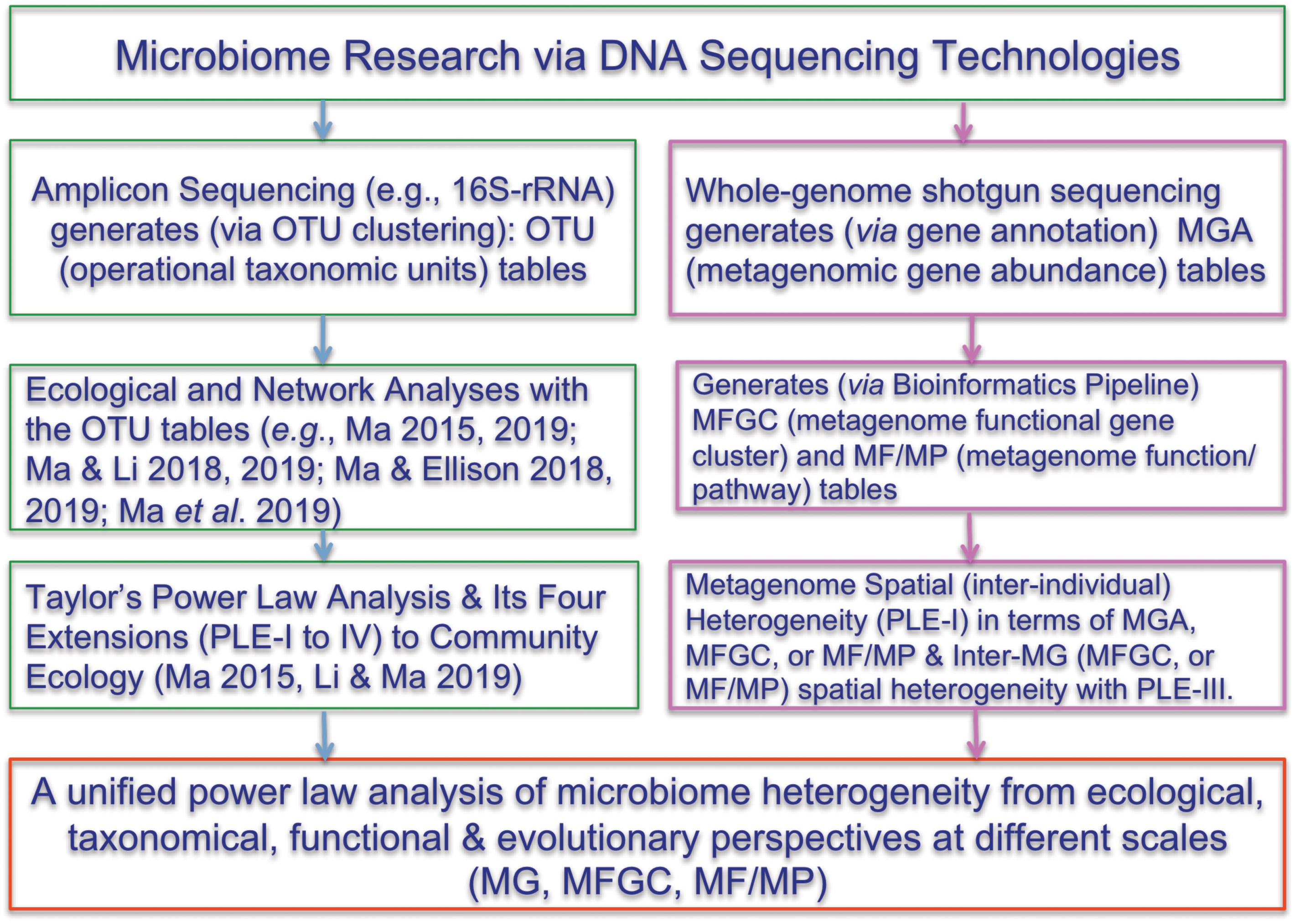
Figure 1. Showing the flowchart of analyzing the microbiome heterogeneity from ecological, taxonomical, functional and evolutionary perspective in terms of various scales [OTU, MG (metagenomic gene), MFGC (metagenome functional gene clusters), MF/MP (metagenomic function/pathway) with the power law extensions (PLEs)]. The right side and framed in red color are newly introduced in the present study. See the Online Supplementary Information (OSI) for the R-Scripts implementing the PLE analysis and randomization tests.

Taylor’s (1961) power law, describing the scaling relationship between the population mean abundance (m) and its variance (V) over space (i.e., V = a^mb), is one of few well recognized ecological laws in population ecology, and it offers a powerful mathematical tool to measure the spatial aggregation (heterogeneity). Its power law scaling parameter (b) often embodies rich ecological and evolutionary insights about specie abundance and distribution over space or time across different environments (Taylor, 1961, 1984, 2007; Taylor and Taylor, 1977; Taylor et al., 1983, 1988). Since its discovery more than a half century ago (Taylor, 1961), Taylor’s power law has been the target of numerous field tests and theoretical analyses, especially in macrobial ecology of plants and animals. In particular, a resurgence of theoretical investigation and extensions to even wider applications in many fields of science and technology, particularly inter-disciplinary studies, has been ongoing in the last few years (e.g., Reuman et al., 2009, 2014, 2017; Cohen et al., 2012, 2013; Ma, 2012, 2015; Stumpf and Porter, 2012; Wearn et al., 2013; Cohen, 2014; Zhang et al., 2014; Cohen and Xu, 2015; Cohen and Saitoh, 2016; Oh et al., 2016; Tippett and Cohen, 2016; Quist et al., 2017). In a previous study (Ma, 2015), we extended the original Taylor’s (1961) power law from population to community level and tested four power law extensions (PLEs) with the 16s-rRNA amplicon-sequencing datasets of the microbial communities from the human microbiome project (Human Microbiome Project Consortium [HMP]). Among the four PLEs introduced by Ma (2015), Type-I and Type-III PLEs can quantify the community (level) spatial heterogeneity and mixed-species (level) spatial heterogeneity, respectively. Type-II and Type-IV were proposed to assess the community temporal stability and mixed-species temporal stability, respectively, but this study does not implicate them since both Type-II and IV require time-series data, for which we did not get sufficiently large datasets, but they should still be applicable for measuring the metagenome stability.

PLE-I (Type-I Power Law Extension) for Measuring Metagenome Spatial Heterogeneity

Similar to the PLE-I for measuring community spatial heterogeneity (Ma, 2015), we propose to use the following mean-variance power function for measuring the metagenome spatial heterogeneity of a metagenome assemblage (or meta-metagenome, as explained previously):

$$V_s=a{m}_s^b\mathit{\hspace{1em}}s=1,2,\mathrm{\dots },S(1)$$

where m_s is the mean of gene abundances of all genes (species) (G) in the metagenome of an individual subject (s = 1, 2, …S), V_s is the corresponding variance, S is the number of subjects, and G is the number of genes contained in the metagenomes of the S subjects. Note m_s is the mean gene abundance per gene species, not per subject, which is different from the case in PLE-III (type-III power law extension) introduced below. In addition, the fitting of Eqn. (1) is performed with S data points, i.e., across S individual subjects (or S metagenomes), rather than across genes, as in the case of PLE-III below.

The parameter b describes the fractional scaling of V-m relationship statistically, or the metagenome spatial heterogeneity biologically. When b = 1, the heterogeneity is random, which means that the heterogeneity—the inter-subject difference in their gene abundance distribution—is essentially random, statistically follows Poisson distribution. When b > 1, the inter-subject heterogeneity is non-random and follows highly skewed long-tail distribution (such as the power law distribution). When b < 1, the inter-subject heterogeneity in their metagenome is fixed, or follows the uniform statistical distribution. From field studies in ecology, the cases when b = 1 or b < 1 are extremely rare in real world and usually only exist theoretically (Taylor, 1961, 1984). We term a metagenome assemblage (i.e., an assemblage of metagenomes) with b = 1 random metagenome (strictly speaking, metagenome assemblage), b < 1, homogenous metagenome, and b > 1, heterogeneous metagenome.

Parameter a in Eqn. (1) is meanwhile related to sampling related factors such as sampling unit or sequencing platforms, but is little influenced by biological interactions. Hence, we generally do not attempt to draw biological interpretations from parameter a due to the strong influence from sampling. It is noted that parameter a also has the same interpretation in PLE-III below.

We further define critical diversity of metagenome heterogeneity (CDMH) or m₀ as:

$$m_0=\exp [\ln (a)/(1-b)]\mathit{\hspace{1em}}(b\ne 1)(2)$$

where a and b are PLE-I parameters from eqn. (1). The CDMH or m₀ is the mean gene abundance level (per gene species) at which metagenome spatial heterogeneity is random, and across which the heterogeneity transits to either heterogeneous (when m > m₀) or regular (uniform or fixed) (when m < m₀). Since the mean gene abundance, although termed abundance, is essentially a measure of gene diversity (i.e., the mean abundance of various gene species in a metagenome), we used the term critical diversity of metagenome heterogeneity, rather than using the term “critical abundance.” The latter is indeed used in the next section for PLE-III, which is the average of single gene abundances from various individuals and consequently the term abundance is more appropriate.

PLE-III (Type-III Power Law Extension) for Measuring Gene-Level Spatial Heterogeneity

Similar to the PLE-III for measuring mixed-species spatial heterogeneity in Ma (2015), we propose to use the following mean-variance power function for measuring the gene-level (inter-gene, or mixed-gene) spatial heterogeneity:

$$V_g=a{m}_g^b\mathit{\hspace{1em}}g=1,2,\mathrm{\dots },G(3)$$

where m_g is the mean abundance of g-th gene, averaged across S subjects (g = 1, 2, …G), V_g is the corresponding variance, and G is the number of gene kinds (gene species), and S is the number of individual subjects sampled. Note m_g is the mean gene abundance of the g-th gene species per subject (not per gene), which is opposite from the case in the previously introduced PLE-I for measuring metagenome spatial heterogeneity. In addition, the fitting of Eqn. (3) is performed with G data points, i.e., across all G gene species, rather than across S subjects, as in the case of the previous PLE-I.

Note that the notion of “mixed-gene” is similar to the concept of mixed-species population in the original Taylor’s power law (Taylor and Woiwod, 1982; Taylor, 1984). It refers to a virtually “averaged assemblage” of genes, in which the identities or kinds of different genes were ignored. The m-V pairs are regressed (see below, through log-linear transformation into linear regression) across multiple gene species (millions in the case of this study) in a mixture manner. Given that the notion of gene species is not widely used in metagenomic research, we suggest using the term gene-level or inter-gene heterogeneity, rather than mixed-gene heterogeneity in the context of PLE-III.

When b = 1, the heterogeneity among metagenomic genes in terms of their gene abundance distributions should be random, i.e., all genes in the metagenome are equivalent to each other in terms of their abundance distribution, similar to the neutrality assumption in the neutral theory of biodiversity. When b < 1, the heterogeneity or difference among genes, if any, should be fixed, or follow a uniform distribution statistically. Both the cases of b = 1 or b < 1 should be extremely rare in real world, and are mostly theoretical possibilities. In practice, b > 1 should be the norm rather than the exception for metagenome heterogeneity at the gene-level. When b > 1, we say the metagenome is heterogeneous or aggregated in terms of its gene-level or inter-gene heterogeneity.

We further define critical abundance of gene-level heterogeneity (CAGH) or m₀ as:

$$m_0=\exp [\ln (a)/(1-b)]\mathit{\hspace{1em}}(b\ne 1)(4)$$

where a and b are PLE-III parameters from eqn. (3). The CAGH or m₀ is the mean gene abundance level (per individual or sample) at which gene-level spatial heterogeneity is random, and across which the heterogeneity transits to either heterogeneous (when m > m₀) or regular (uniform or fixed) (when m < m₀).

Statistical Fitting of PLE-I or PLE-III

To fit the power law, including PLE-I and PLE-III, the most commonly used approach is to transform the power law model [eqn. (1) or (3)] into the following linear function:

$$\ln (V)=\ln (a)+b\ln (m)(5)$$

where all the variables (m, V) and parameters (a, b) have the exactly same interpretations as those in eqn. (1) or eqn. (3). Standard linear regression procedure can be applied to fit the model. In fact, there is an advantage for adopting the simple linear transformed regression approach, which is related to an important property of power law, scale-invariance. This property makes parameter a less relevant for determining the most important parameter of power law, i.e., the scaling parameter b (Ma, 2015). It is for this reason that we choose the simple linear regression approach for fitting all the power law models. This allows us to focus on the scaling parameter (b) for assessing and interpreting the metagenome heterogeneity revealed by the metagenomic sequencing data.

As a side note, we may define metagenome temporal stability with Type-II PLE or gene-level temporal stability with Type-IV PLE, similar to Ma (2015) for community temporal stability or mixed-species temporal stability, but their demonstrations require time-series MGA data obtained with metagenomic (whole-genome or shotgun) sequencing technologies. We failed to find sufficiently long time-series MGA data to demonstrate the PLE-II or PLE-IV models and won’t further discuss the temporal versions of the PLE in this study (Nielsen et al., 2014).

Bioinformatics Analysis of Metagenomic Sequencing Data

To fit the power law model, one has to first compute MGA tables from metagenomic sequencing raw reads (also known as shotgun or whole-genome sequencing) by using standard bioinformatics software pipelines (e.g., Li and Godzik, 2006; Qin et al., 2010, 2012; Zhu et al., 2010; Chatelier et al., 2013; Li et al., 2014; Xiao et al., 2015, 2016; Wang and Jia, 2016; Sczyrba et al., 2017; Ma and Li, 2018).

Millions of contigs are obtained through the metagenome assembly step. Those millions of contigs are fed into gene prediction software and the latter generate a list of non-redundant genes based on the criteria set by ORFs (open reading frames). We term those non-redundant genes as metagenomic genes (MGs) or simple genes. MG embodies single-gene-level genetic information, and its number in a typical metagenome sample is in the magnitude of millions (Ma and Li, 2018). The previously defined MGA table is actually the table of MGs.

Directly characterizing or summarizing information from the millions of MGs or MGA tables can be rather challenging. An alternative research strategy is to first group those millions of genes (MGs) into functional gene clusters, and then investigate the properties of the functional gene clusters. There are mature bioinformatics algorithms and software pipelines to cluster the millions of MGs into hundreds of MFGCs (metagenome functional gene clusters), and the magnitude of MFGC numbers (hundreds) is much small that that of the MGs (millions) (Ma and Li, 2018). Obviously, the huge reduction in the magnitudes from MGs (millions) to MFGCs (hundreds) should make our measuring metagenomic spatial heterogeneity simpler.

Demonstration and Discussion

The Datasets of Metagenomes

We collected three gut metagenome datasets from public domain including, 264 stool samples from overweight and lean individuals (Qin et al., 2010; Chatelier et al., 2013), 145 stool samples from type-2 diabetes and healthy controls (Qin et al., 2012), and 219 stool samples from IBD patients and healthy controls. A total of 628 metagenome samples with their metagenomic gene (MG) catalog and the gene abundance (MGA) tables for each dataset were computed with standard metagenomic analysis pipelines (e.g., Li and Godzik, 2006; Qin et al., 2010, 2012; Zhu et al., 2010; Chatelier et al., 2013; Li et al., 2014; Xiao et al., 2015, 2016; Wang and Jia, 2016; Sczyrba et al., 2017). Furthermore, we defined metagenome functional gene clusters (MFGC) based on Ma and Li (2018) and obtained their abundance tables. Supplementary Table S1 showed more detailed information about the three datasets we use in this paper for demonstrating the application of the power law.

Specifically, after whole-genome (shotgun) sequencing of a metagenome sample, sequencing reads from the fecal samples were processed for quality control, removal of human sequences, assembling, assembly revision and gene prediction by using MOCAT pipeline (Kultima et al., 2012). This pipeline consists of a series of software packages, which can process metagenomes in a standardized and automated manner while improving the quality of assembly and gene prediction at run time. In the pipeline, FASTX Toolkit¹ was used for quality control; SOAPaligner2 (Li et al., 2009) for identifying human sequences; SOAPdenovo v1.06 (Li et al., 2010) for assembling; MetaGeneMark (Zhu et al., 2010) for gene prediction; CD-HIT (Li and Godzik, 2006) for clustering genes in each cohort.

The details of the data/software/parameters used to compute the MGA tables can be found in the online method of Li et al. (2014). In fact, the MGA tables are available online at: http://meta.genomics.cn/meta/dataTools. Li et al. (2014) annotated the metagenomic genes according to the “Kyoto Encyclopedia of Genes and Genomes” (KEGG) and the “evolutionary genealogy of genes non-supervised orthologous groups” (eggNOG) databases. They further identified a total of 6,980 KEGG orthologous groups (KOs) and 36,489 eggNOG orthologous groups, accounting for 51.6 and 69.3% of the total sequencing reads.

In the online Supplementary Information (OSI), the R-Scripts for implementing the power law analysis and randomization tests for determining the differences in the PLE parameters are provided.

Metagenome Spatial Heterogeneity in Terms of the MGA (Metagenomic Gene Abundance) Spatial (Inter-Subject) Distribution Measured With PLE-I

We first fitted PLE-I (type-I power law extension) with metagenomic gene abundance (MGA) datasets directly in order to measure the metagenome spatial (inter-subject) heterogeneity for each treatment (group) of the three datasets, and the results were listed in Table 1, from which we summarize the following findings:

TABLE 1

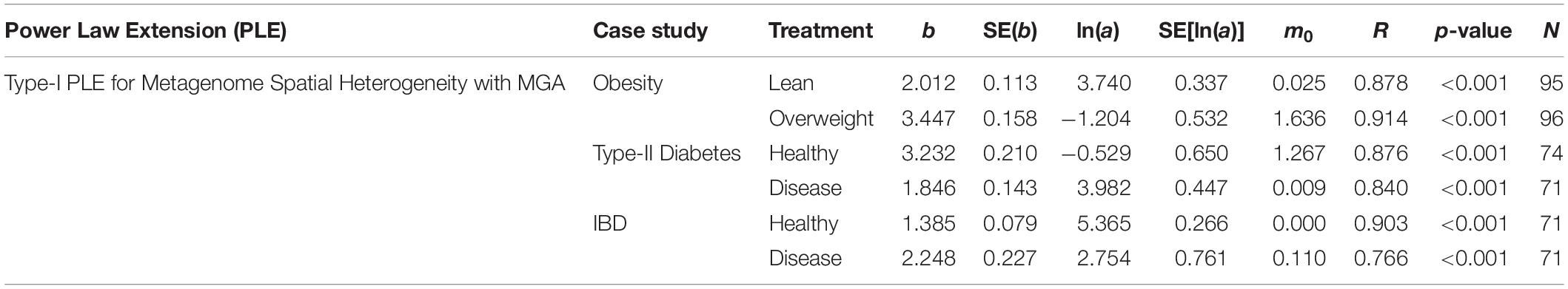
Table 1. The parameters of PLE-I (type-I power law extension) for metagenome spatial heterogeneity, in terms of the MGA (metagenomic gene abundance).

(i) PLE-I fitted to all three datasets extremely well with p-value < 0.0001. This indicates the ubiquitous applicability of the PLE for assessing the metagenome spatial (i.e., inter-subject) heterogeneity of either MGA (this section) or MFGC (the next section).

(ii) The scaling parameter (b) of PLE-I for the most treatments is between 2 and 4 except for the two treatments (diseased treatment in the diabetes study, and the healthy treatment in the IBD study), and the parameter (b) varied significantly between the treatments with a range of [1.385, 3.447].

(iii) The values of the scaling parameter (b) for the healthy samples (group) and diseased samples (group) were significantly different (p-value < 0.05), in all three case studies (obesity, diabetes and IBD). Therefore, we conclude that PLE-I can be harnessed to measure the metagenome spatial heterogeneity in terms of gene abundance distribution. Furthermore, it has a potential being a discriminant metric for distinguishing between the healthy and diseased metagenome samples, as revealed in Table 2 (p-value < 0.05), in which randomization test (Collingridge, 2013) with 1000 times of re-sampling was utilized to test the difference in the b-value between the healthy and diseased treatments. Figure 2 shows the fitted power law models for the obesity case study, i.e., one straight line for the lean group and another for the overweight group.

TABLE 2

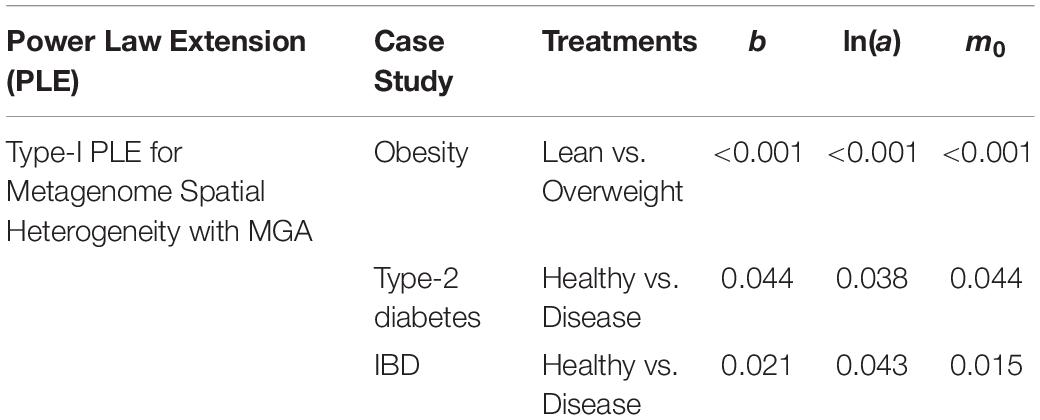
Table 2. The p-value of the randomization test for the difference between the healthy and diseased treatments in their metagenome spatial heterogeneities parameters of PLE-I.

FIGURE 2

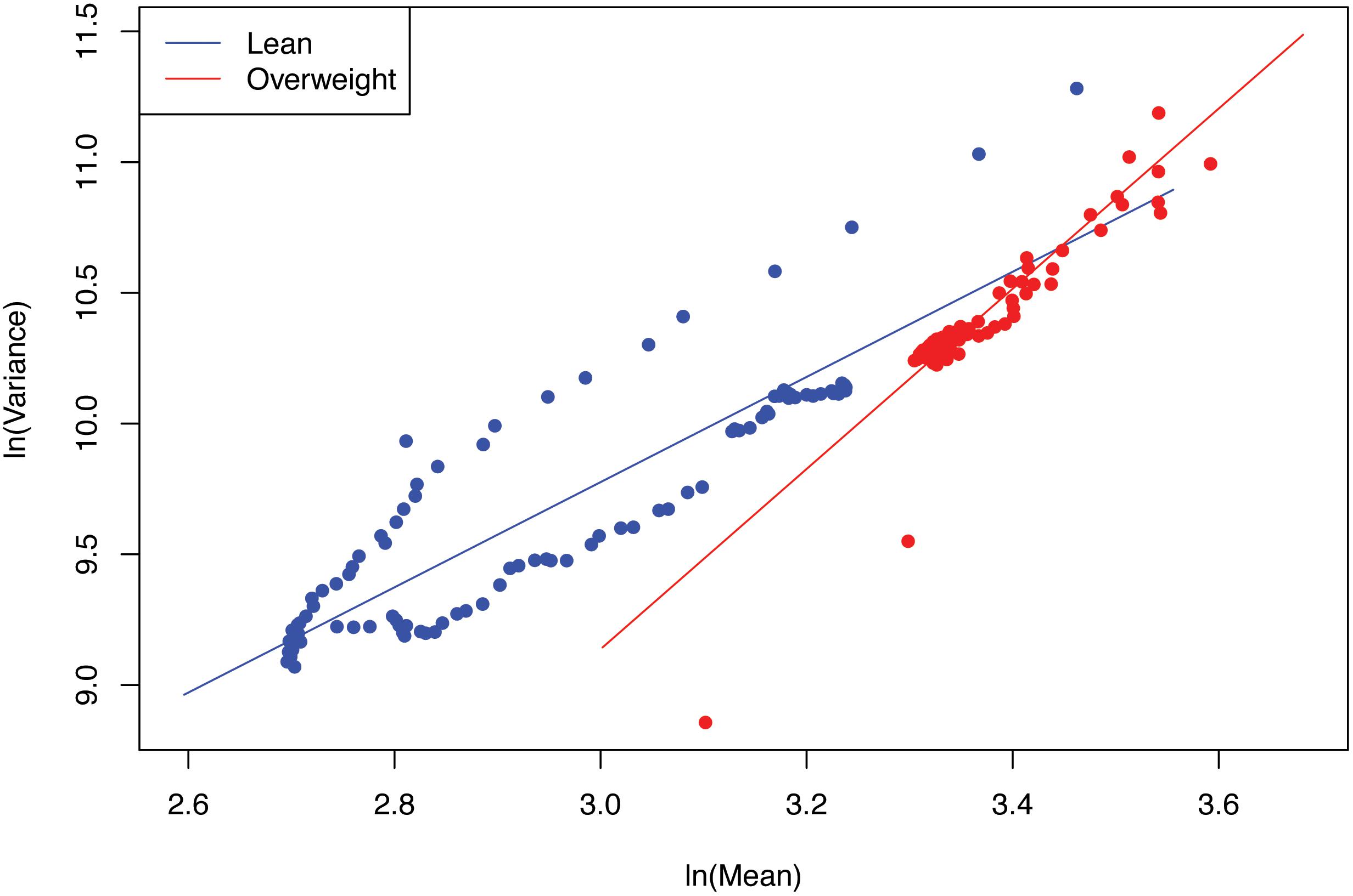
Figure 2. The PLE-I (type-I power law extension) models fitted for the obesity case study.

The metagenome spatial heterogeneity is the counterpart of community spatial heterogeneity in community ecology, and it measures the spatial heterogeneity of metagenomes of individual subjects or inter-subject metagenome heterogeneity in a population (or cohort), similar to measuring the heterogeneity among spatially explicit local communities in community ecology (Ma, 2015). With our newly coined term of metagenome assemblage, parameter b measures the heterogeneity of metagenome assemblage represented by a MGA table. The higher b-value of PLE-I represents greater heterogeneity (unevenness or diversity) among individuals in their metagenomes in terms of their gene abundance distributions. When b = 1, it implies that the differences among individuals are random. When b < 1, it implies that the differences among individuals follow uniform distribution statistically (i.e., a fixed difference).

Gene-Level (or Inter-Gene) Spatial Heterogeneity in Terms of the MGA (Metagenomic Gene Abundance) Distribution Measured With PLE-III

We also fitted the PLE-III (type-III power law extension) with metagenomic gene abundance (MGA) datasets directly in order to measure the gene-level or mixed-gene spatial heterogeneity for each of the 3 datasets, and the results were listed in Table 3 below. It was shows that:

TABLE 3

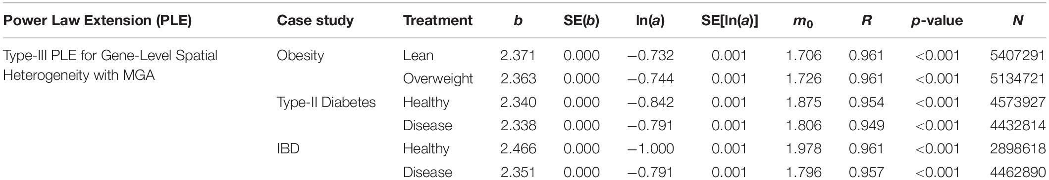
Table 3. The parameters of PLE-III (type-III power law extension) for measuring gene-level (inter-gene) spatial aggregation, in terms of the metagenomic gene abundance (MGA).

(i) The PLE-III fitted to all 3 datasets extremely significant with p-value < 0.0001, and the standard errors of the model parameters were close to zero. The linear correlation coefficients were between 0.949 and 0.961. All the criteria indicate that the goodness-of-fitting to PLE-III was extremely well given millions of data points were fitted.

(ii) The parameter b of PLE-III for all the treatments fall in a rather narrow range of [2.340, 2.466]. Therefore, we conclude that PLE-III can be harnessed to measure the gene-level spatial heterogeneity in terms of the gene abundance distribution, but its application for discriminating the healthy and diseased samples is of limited value given its insensitivity to host factors such as diseases. Figure 3 shows the fitted PLE-III with the dataset from the obesity study.

FIGURE 3

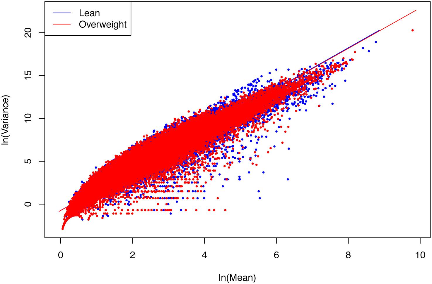
Figure 3. The PLE-III (type-III power law extension) models fitted to the obesity study datasets: more than 10 million points (5407291 lean group + 5134721 overweight) were used to fit the PLE-III models, but here we only randomly selected 100,000 points (50,000 from each treatment) to draw the graphs (so as to accommodate the file size of the figure).

Taylor’s power law has been tested with hundreds, if not thousands, of field studies and many theoretical examinations (Taylor, 1961, 1981, 1984, 2007; Taylor et al., 1983, 1988; Ma, 1991, 2012, 2013, 2015, 2018; Reuman et al., 2009, 2014, 2017; Stumpf and Porter, 2012; Cohen and Xu, 2015; Tippett and Cohen, 2016; Quist et al., 2017). However, to the best of our knowledge, the tests exhibited in Table 3 should be the cases that have used the biggest numbers of data points (the column N in Table 3) to fit the power law model, since it was first discovered more than a half century ago. For example, in the case of obesity study, for each of the two treatments (lean vs. overweight), more than five million genes were used to fit PLE-III model. This shows the exceptional robustness of the power law model.

The PLE-III for measuring the gene-level or mixed-gene spatial heterogeneity is the counterpart of mixed-species spatial aggregation in community ecology (Ma, 2015). The term aggregation is often used in population ecology, and it is the counterpart of heterogeneity in community ecology. As explained previously, the term mixed-gene setting assumes that we ignore the identities of individual genes, and what is measured is the aggregation (unevenness or heterogeneity) of an average gene species. We suggest using the term “gene-level spatial heterogeneity” for what is measured with the PLE-III in metagenomic research.

Metagenome Spatial Heterogeneity in Terms of the MFGC (Metagenome Functional Gene Cluster) Distribution Measured With PLE-I

According to Ma and Li (2018), the term MFGC (metegenome functional gene cluster) refers to cluster of functionally similar or same genes, generated from functional annotation or gene annotation through online mapping to functional databases such as KEGG (for metabolic pathways) and eggNOG (for protein functions). Hence, MFGC is purely functionality-based and is mostly cross-species. One of its unique advantages is that it embodies the functional redundancy in microbiome very well. The difference between Type-I MFGC (MFGC-I) and Type-II MFGC (MFGC-II) lies in their differences in handling the genes within each cluster. In MFGC-I, only the number of gene species (kinds) is counted but the abundance of individual gene is ignored. In MGGC-II, both the number of gene species (kinds) and the abundance of each gene matter in the analysis. In other words, with MFGC-I, we only care the number of gene species (kinds), and with MFGC-II we care both the number of gene species (kinds) and the abundance of each gene within each cluster. This treatment is very similar to a common practice in community ecology, where a simplified measure for biodiversity is to only count the number of species (also known as species richness), and a more comprehensive measure of biodiversity uses more sophisticated entropy such as Shannon entropy, which consider both species richness and abundances.

In the previous section, we conducted power law analysis in terms of the metagenomic gene (MG) or metagenomic gene abundance (MGA) distribution. In this section, our analysis is performed in terms of the metagenome functional gene cluster (MFGC). That is, using the MFGC abundance tables (similar to MGA or OTU tables, except that the entity is the MFGC) to fit the PLE models.

The results of fitting the PLE-I with MFGC tables were listed in Table 4, from which we can observe the following findings:

TABLE 4

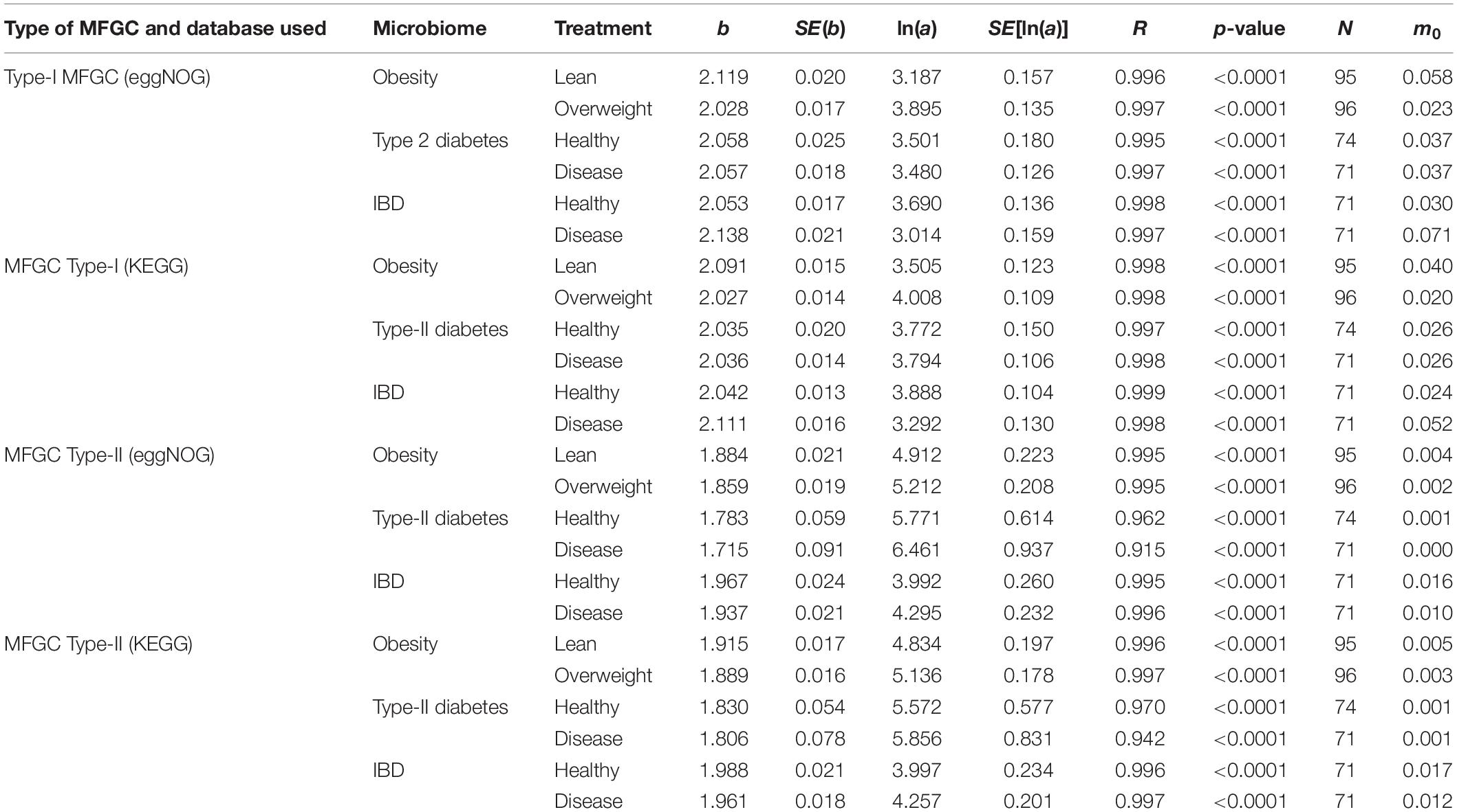
Table 4. The parameters of PLE-I (type-I power law extension) for metagenome spatial heterogeneity, in terms of the MFGC (metagenome functional gene cluster) distribution.

(i) The PLE-I model fitted to the MFGC abundances extremely well (significant with p-value < 0.0001), and this indicates the ubiquitous applicability of the PLE for assessing the metagenome spatial (i.e., inter-subject) heterogeneity of either MFGCs (this section) or MG (previous section).

(ii) MFGC-I and MFGC-II exhibited slightly different scaling parameter (b) values. The scaling parameter b of PLE-I ranged [2.027, 2.138] for MFGC-I and [1.715, 1.988] for MFGC-II, indicating that the MFGC-I has a higher heterogeneity degree. This difference should be due to their definitional difference: MFGC-I ignored the information of individual gene abundances, only taking into account the number of gene species (kinds), or gene richness. Obviously, ignoring the gene abundance information should lead to larger heterogeneity (difference), which explains why the PLE-I parameter b of MFGC-I was slightly higher (b > 2), while that of MFGC-II was lower (b < 2). Furthermore, MFGC-II should better embody functional redundancy information given that it considers both gene species (kinds or richness) and abundances.

(iii) Although MFGC-I and MFGC-II displayed slightly different ranges in their parameter b, the b-values from two databases (eggNOG and KEGG) within each MFGC type were rather close with each other and the difference was negligible. This simply indicates that the heterogeneity scaling based on metabolic pathways (KEGG database) or protein functions (eggNOG) makes little difference. This should be expected given that, at the MFGC level, both eggNOG and KEGG should be controlled by the same underlying gene-level mechanisms.

(iv) As shown in Table 5, in terms of the parameter changes associated with diseases, only IBD treatment displayed significant difference from its healthy control in MFGC-I, and the other diseases treatments did not exhibit any significant differences from their healthy controls. This result suggests that at the MFGC level, the metagenome spatial heterogeneity is less sensitive to diseases than at the MG level, as indicated by the randomization test results in Table 2.

TABLE 5

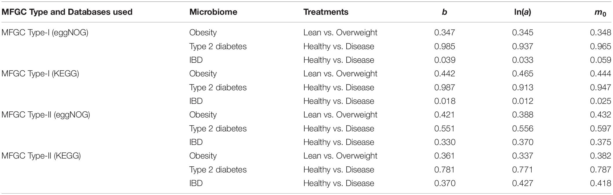
Table 5. The p-value of the randomization test for the difference between the healthy and diseased treatments in their PLE-I (type-I power law extension) parameters in terms of the MFGC.

MFGC-Level (Inter-MFGC) Spatial Heterogeneity in Terms of the MFGC (Metagenome Functional Gene Cluster) Distribution Measured With PLE-III

In the previous section, we investigated the spatial heterogeneity of MFGC by using the PLE-I (type-I power law extension) modeling. That is to analyze the inter-subject heterogeneity of their metagenomes in terms of the functional gene cluster (i.e., MFGC). In this section, we investigate the spatial heterogeneity at the MFGC-level by using PLE-III (type-III power law extension). In other words, by assuming that there exists an average MFGC in a mixed-MFGC setting (by ignoring the difference among MFGCs), we assess the heterogeneity of MFGCs at the average MFGC level. Therefore, a fundamental difference between the analysis here and the analysis in the previous section is that here, the heterogeneity is measured in terms of a virtually averaged MFGC (or at MFGC-level), while in the previous section, the heterogeneity was measured in terms of the whole metagenome (or at metagenome level).

To save page space, the results for MFGC-level spatial heterogeneity were listed in Supplementary Table S2 in the OSI (online Supplementary Information), from which we summarize the following findings:

(i) The PLE-III model fitted to the MFGC tables extremely significant with p-value < 0.0001 in all three case studies, and this indicates the ubiquitous applicability of the PLE for assessing the spatial (i.e., inter-subject) heterogeneity of an ‘averaged’ MFGC.

(ii) The scaling parameter (b) of the PLE-III model ranged narrowly [1.472, 1.654], and varied little either between the MFGC-I and MFGC-II or between the healthy and diseased treatments within each case study. This suggests that, the sensitivity of the scaling parameter (b) of PLE-III to host factors such as diseases is rather muted, and consequently may be of limited practical applications.

(iii) Contrary with the pattern of PLE-I in the previous section, where MFGC-I has slightly larger scaling parameter (b) value than MFGC-II has, here MFGC-I [1,472, 1.547] has slightly smaller b-value than MFGC-II [1.525, 1.654] does.

(iv) The scaling parameter (b) of PLE-III, estimated with KEGG or eggNOG showed little differences, similar with the previous PLE-I model.

(v) We also performed the randomization tests for the PLE-III parameters (Supplementary Table S3). In most cases, the model parameters did not showed significant differences between the healthy and diseased treatments.

Conclusion and Discussion

In previous sections, we demonstrated that PLE-I and PLE-III, originally designed to measure community spatial heterogeneity and mixed-species population spatial aggregation in community ecology (Taylor, 1961, 1984; Ma, 2015), can be introduced to (i) measure metagenome spatial heterogeneity in terms of either MG or MFGC abundance distribution and measured with PLE-I; or (ii) MG-level (or MFGC-level) spatial heterogeneity measured with PL-III. The first application is a measure at the whole metagenome (more accurately, metagenome assemblage) level, because it measures the inter-subject (spatial) heterogeneity within a cohort or population of individuals in their metagenomes. The second application is a measure at MG or MFGC level, because it measures the inter-MG or inter-MFGC heterogeneity from the perspective of a virtually averaged MG or MFGC. Although we used the metagenomic datasets of the human microbiome to demonstrate the concepts and modeling analyses, the approaches should be equally applicable to the metagenomes of other microbiomes on the planet.

Traditionally, studies on heterogeneity have been mostly focused on population level, and metrics for community heterogeneity are relatively fewer. This may be to do with that community level studies are mostly focused on community diversity, instead. Nevertheless, heterogeneity and diversity are not the same (Shavit et al., 2016). First, the heterogeneity is a “group” property, while diversity can be measured with one individual or single community. Without comparing two entities, heterogeneity does not make sense. Second, diversity is a measure of numbers (and relative abundances), while heterogeneity needs to be measured by interactions and working together (Shavit et al., 2016). For example, one may say, “zoos are diverse, and natural ecosystems are heterogeneous” (Ayelet Shavit and Aaron Ellison, personal communication, 22 April 2020).

Two additional heterogeneity indexes that can be used to measure community level heterogeneity are: (i) Variance/mean ratio (V/m) and (ii) community dominance index M^∗/m. Both are counterparts of spatial aggregation index and patchiness index at the population level in population ecology (Taylor, 1984; Ma, 1991). Both indexes have different definitions and interpretations. The V/m heterogeneity index is simply a ratio of the mean species abundances (m) and corresponding variance (V), and a larger index value indicates higher heterogeneity (Taylor, 1984; Ma, 1991). The community dominance index (D_c) was defined by Ma and Ellison (2018), and a larger index value indicates lower heterogeneity. Table 6 shows the values of the computed heterogeneity indexes for the three datasets (see Supplementary Table S1) we used, as well as the p-values from Wilcoxon tests for the differences between the healthy and diseased treatments in each of the three datasets.

TABLE 6

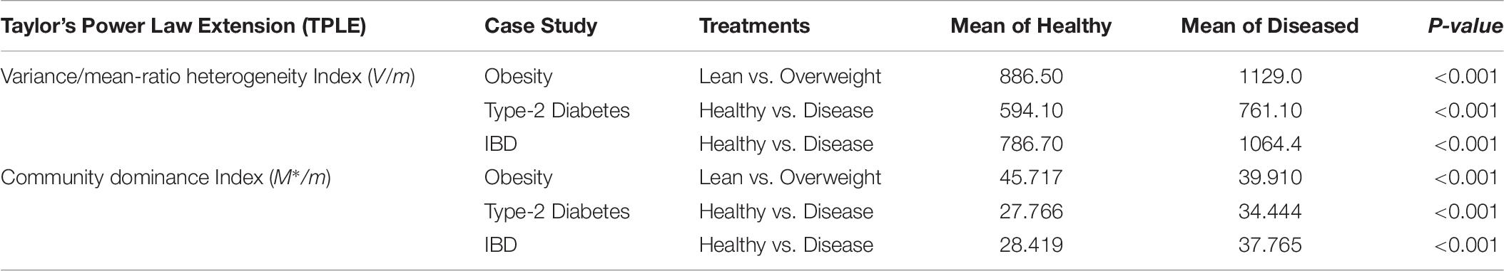
Table 6. The p-value of Wilcoxon tests for the difference between the healthy and diseased treatments in their metagenome spatial heterogeneities and community dominance (also see Supplementary Figure S1A for the V/M heterogeneity index and Supplementary Figure S1B for the community dominance index).

Obviously, the two heterogeneity indexes described above are much simpler to implement than the power law modeling introduced in this study. Furthermore, both indexes displayed significant differences between the healthy and diseased treatments in their metagenome heterogeneity. Given their simplicity, a natural question is: what are the advantages from using the power law modeling? The answer is that the power law analysis we presented offers tools to synthesize and measure the heterogeneity at various scales (MG, MFGC) across individuals in a cohort (population), with a unified power law model, which achieved the rare status of classic ecological laws. In fact, the power law analysis demonstrated here can also be applied to measure metagenome temporal stability at similar scales to the previous spatial versions. Furthermore, the power law analysis provides a unified modeling tool to assess and interpret the heterogeneity from ecological, taxonomical, functional and evolutionary perspectives, because it can be applied to both OTU tables and MGA tables, with the exactly same mathematical model (the power law model). When using MGA tables, it can be universally applied to the scales of the metagenomic gene or metagenome functional gene cluster.

Perhaps an even more compelling case for using the TPL/PLE parameters rather than the simple heterogeneity indexes has to do with the difference between heterogeneity and diversity. As argued previously, heterogeneity is a “group” property; measuring heterogeneity requires at least two entities. While TPL/PLE can synthesize the information from potentially unlimited number of entities (samples), the two heterogeneity indexes previously introduced were computed from single sample. To synthesize information from multiple samples, additional statistics such as the mean of the heterogeneity values, as displayed in Table 6, must be used. Nevertheless, the distribution of heterogeneity values may satisfy the Gaussian distribution. This may make the usage of mean problematic since the distribution of heterogeneity per se is usually highly skewed and follows power law distribution. In addition, it may even argue that the two simple heterogeneity indexes are similar to diversity measures. For example, the community dominance (M^∗/m), as heterogeneity index, may even be treated as the other side of the evenness (diversity) coin (Ma and Ellison, 2018).

Data Availability Statement

The datasets analyzed in this manuscript are publically available for downloading and the sources were noted in Supplementary Table S1.

Author Contributions

ZM designed the study, conducted the study and wrote the manuscript.

Conflict of Interest

The author declares that the research was conducted in the absence of any commercial or financial relationships that could be construed as a potential conflict of interest.

Acknowledgments

This study received funding from the following sources: A National Natural Science Foundation of China (NSFC) Grant (No. 31970116) on the Medical Ecology of Human Microbiome; The Cloud-Ridge Industry Technology Leader Award; An International Cooperation Grant (YNST) on Genomics & Metagenomics Big Data. The funders played no roles in interpreting the results.

Supplementary Material

The Supplementary Material for this article can be found online at: https://www.frontiersin.org/articles/10.3389/fmicb.2020.00648/full#supplementary-material

Footnotes

1. ^ http://hannonlab.cshl.edu/fastx_toolkit/

References

Barberaìn, A., Casamayor, E. O., and Fierer, N. (2014). The microbial contribution to macroecology. Front. Microbiol. 5:203. doi: 10.3389/fmicb.2014.00203

PubMed Abstract | CrossRef Full Text | Google Scholar

Chatelier, E. L., Nielsen, T., Qin, J., Prifti, E., Hildebrand, F., Falony, G., et al. (2013). Richness of human gut microbiome correlates with metabolic markers. Nature 500, 541–546.

Google Scholar

Cohen, J. E. (2014). Taylor’s law and abrupt biotic change in a smoothly changing environment. Theor. Ecol. 7, 77–86. doi: 10.1007/s12080-013-0199-z

CrossRef Full Text | Google Scholar

Cohen, J. E., and Saitoh, T. (2016). Population dynamics, synchrony, and environmental quality of Hokkaido voles lead to temporal and spatial Taylor’s laws. Ecology 97:3402. doi: 10.1002/ecy.1575

PubMed Abstract | CrossRef Full Text | Google Scholar

Cohen, J. E., and Xu, M. (2015). Random sampling of skewed distributions implies Taylor’s power law of fluctuation scaling. Proc. Natl. Acad. Sci. U.S.A. 112:7749. doi: 10.1073/pnas.1503824112

PubMed Abstract | CrossRef Full Text | Google Scholar

Cohen, J. E., Xu, M., and Schuster, W. S. (2013). Stochastic multiplicative population growth predicts and interprets Taylor’s power law of fluctuation scaling. Proc. Biol. Sci. 280:20122955. doi: 10.1098/rspb.2012.2955

PubMed Abstract | CrossRef Full Text | Google Scholar

Cohen, J. E., Xu, M., and Schuster, W. S. F. (2012). Allometric scaling of population variance with mean body size is predicted from Taylor’s law and density-mass allometry. Proc. Natl. Acad. Sci. U.S.A. 109:15829. doi: 10.1073/pnas.1212883109

PubMed Abstract | CrossRef Full Text | Google Scholar

Collingridge, D. S. (2013). A primer on quantitized data analysis and permutation testing. J. Mixed Methods Res. 7, 79–95.

Google Scholar

Costello, E. K., Stagaman, K., Dethlefsen, L., Bohannan, B. J. M., and Relman, D. A. (2012). The application of ecological theory toward an understanding of the human microbiome. Science 336, 1255–1262. doi: 10.1126/science.1224203

PubMed Abstract | CrossRef Full Text | Google Scholar

Hanson, C. A., Fuhrman, J. A., Horner-Devine, M. C., and Martiny, J. B. (2012). Beyond biogeographic patterns: process shaping the microbial landscape. Nat. Rev. Microbiol. 10, 497–506. doi: 10.1038/nrmicro2795

PubMed Abstract | CrossRef Full Text | Google Scholar

Human Microbiome Project Consortium [HMP] (2012). Structure, function and diversity of the healthy human microbiome. Nature 486, 207–214. doi: 10.1038/nature11234

PubMed Abstract | CrossRef Full Text | Google Scholar

Kultima, J. R., Sunagawa, S., Li, J., Chen, W., Chen, H., Mende, D. R., et al. (2012). MOCAT: a metagenomics assembly and gene prediction toolkit. PLoS One 7:e47656. doi: 10.1371/journal.pone.0047656

PubMed Abstract | CrossRef Full Text | Google Scholar

Li, H., and Reynolds, J. F. (1995). On definition and quantification of heterogeneity. Oikos 73:28.

Google Scholar

Li, J., Jia, H., Cai, X., Zhong, H., Feng, Q., Sunagawa, S., et al. (2014). An integrated catalog of reference genes in the human gut microbiome. Nat. Biotechnol. 32, 834–841.

Google Scholar

Li, R., Yu, C., Li, Y., Lam, T. W., Yiu, S. M., Kristiansen, K., et al. (2009). SOAP2: an improved ultrafast tool for short read alignment. Bioinformatics 25, 1966–1967. doi: 10.1093/bioinformatics/btp336

PubMed Abstract | CrossRef Full Text | Google Scholar

Li, R., Zhu, H., Ruan, J., Qian, W., Fang, X., Shi, Z., et al. (2010). De novo assembly of human genomes with massively parallel short read sequencing. Genome Res. 20, 265–272. doi: 10.1101/gr.097261.109

PubMed Abstract | CrossRef Full Text | Google Scholar

Li, W., and Godzik, A. (2006). CD-hit: a fast program for clustering and comparing large sets of protein or nucleotide sequences. Bioinformatics 22, 1658–1659. doi: 10.1093/bioinformatics/btl158

PubMed Abstract | CrossRef Full Text | Google Scholar

Li, W., and Ma, S. Z.-S. (2019). Diversity scaling of human vaginal microbial communities. Zool. Res. 40, 587–594. doi: 10.24272/j.issn.2095-8137.2019.068

PubMed Abstract | CrossRef Full Text | Google Scholar

Lozupone, C. A., Stombaugh, J. I., Gordon, J. I., Jansson, J. K., and Knight, R. (2012). Diversity, stability and resilience of the human gut microbiota. Nature 2012, 220–230. doi: 10.1038/nature11550

PubMed Abstract | CrossRef Full Text | Google Scholar

Ma, Z. S. (1991). Further interpreted Taylor’s Power Law and population aggregation critical density. Trans. Ecol. Soc. China 1, 284–288.

Google Scholar

Ma, Z. S. (2012). Chaotic populations in genetic algorithms. Appl. Soft Comput. 12, 2409–2424. doi: 10.1016/j.asoc.2012.03.001

CrossRef Full Text | Google Scholar

Ma, Z. S. (2013). Stochastic populations, power law and fitness aggregation in genetic algorithms. Fund. Inform. 122, 173–206. doi: 10.3233/fi-2013-787

CrossRef Full Text | Google Scholar

Ma, Z. S. (2015). Power law analysis of the human microbiome. Mol. Ecol. 24, 5428–5445. doi: 10.1111/mec.13394

PubMed Abstract | CrossRef Full Text | Google Scholar

Ma, Z. S. (2018). DAR (diversity–area relationship): Extending classic SAR (species–area relationship) for biodiversity and biogeography. Ecol. Evol. 8, 10023–10038. doi: 10.1002/ece3.4425

PubMed Abstract | CrossRef Full Text | Google Scholar

Ma, Z. S. (2019). A new DTAR (diversity–time–area relationship) model demonstrated with the indoor microbiome. J. Biogeogr. 46, 2024–2041. doi: 10.1111/jbi.13636

CrossRef Full Text | Google Scholar

Ma, Z. S., and Ellison, A. M. (2018). A unified concept of dominance applicable at both community and species scale. Ecosphere 9:e02477. doi: 10.1002/ecs2.2477

CrossRef Full Text | Google Scholar

Ma, Z. S., and Ellison, A. M. (2019). Dominance network analysis provides a new framework for studying the diversity-stability relationship. Ecol. Monogr. 89:e01358. doi: 10.1002/ecm.1358

CrossRef Full Text | Google Scholar

Ma, Z. S., Li, L., and Gotelli, N. J. (2019). Diversity-disease relationships and shared species analyses for human microbiome-associated diseases. ISME J. 13, 1911–1919. doi: 10.1038/s41396-019-0395-y

PubMed Abstract | CrossRef Full Text | Google Scholar

Ma, Z. S., and Li, L. W. (2018). Measuring metagenome diversity and similarity with Hill numbers. Mol. Ecol. Resour. 18, 1339–1355. doi: 10.1111/1755-0998.12923

PubMed Abstract | CrossRef Full Text | Google Scholar

Ma, Z. S., and Li, W. (2019). How and why men and women differ in their microbiomes: medical ecology and network analyses of the microgenderome. Adv. Sci. 6:1902054. doi: 10.1002/advs.201902054

PubMed Abstract | CrossRef Full Text | Google Scholar

Nielsen, H. B., Almeida, M., Juncker, A. S., Rasmussen, S., Li, J., Sunagawa, S., et al. (2014). Identification and assembly of genomes and genetic elements in complex metagenomic samples without using reference genomes. Nat. Biotechnol. 32, 822–828.

Google Scholar

Oh, J., Byrd, A. L., Park, M., Nisc Comparative Sequencing Program, Kong, H. H., Segre, J. A., et al. (2016). Temporal stability of the human skin microbiome. Cell 165, 854–866. doi: 10.1016/j.cell.2016.04.008

PubMed Abstract | CrossRef Full Text | Google Scholar

Qin, J., Li, R., Raes, J., Arumugam, M., Burgdorf, K. S., Manichanh, C., et al. (2010). A human gut microbial gene catalogue established by metagenomic sequencing. Nature 464, 59–65.

Google Scholar

Qin, J., Li, Y., Cai, Z., Li, S., Zhu, J., Zhang, F., et al. (2012). A metagenome-wide association study of gut microbiota in type 2 diabetes. Nature 490, 55–60.

Google Scholar

Quist, C. W., Gort, G., Mulder, C., Wilbers, R. H. P., Termorshuizen, A. J., Bakker, J., et al. (2017). Feeding preference as a main determinant of microscale patchiness among terrestrial nematodes. Mol. Ecol. 17, 1257–1270. doi: 10.1111/1755-0998.12672

PubMed Abstract | CrossRef Full Text | Google Scholar

Reuman, D. C., Gislason, H., Barnes, C., Mélin, F., and Jennings, S. (2014). The marine diversity spectrum. J. Anim. Ecol. 83, 963–979.

Google Scholar

Reuman, D. C., Mulder, C., and Cohen, J. (2009). Allometry of body size and abundance in 166 food webs. Adv. Ecol. Res. 41, 1–45. doi: 10.1016/S0065-2504(09)00401-2

CrossRef Full Text | Google Scholar

Reuman, D. C., Zhao, L., and Sheppard, L. W. (2017). Synchrony affects Taylor’s law in theory and data. Proc. Natl. Acad. Sci. U.S.A. 114:6788.

Google Scholar

Sczyrba, A., Hofmann, P., Belmann, P., Koslicki, D., Janssen, S., Dröge, J., et al. (2017). Critical assessment of metagenome interpretation-a benchmark of metagenomics software. Nat. Methods 14, 1063–1071.

Google Scholar

Shavit, A., Kolumbus, A., and Ellison, A. M. (2016). Two Roads Diverge in a Wood: Indifference to the Difference Between ‘Diversity’ and ‘Heterogenetiy’ Should Be Resisted on Epistemic and Moral Grounds. Available online at: http://philsci-archive.pitt.edu/12432

Google Scholar

Stumpf, M. P. H., and Porter, M. A. (2012). Critical truths about power laws. Science 335, 665–666. doi: 10.1126/science.1216142

PubMed Abstract | CrossRef Full Text | Google Scholar

Taylor, L. R. (1961). Aggregation, variance and the mean. Nature 189, 732–735. doi: 10.1038/189732a0

CrossRef Full Text | Google Scholar

Taylor, L. R. (1984). Assessing and interpreting the spatial distributions of insect populations. Annu. Rev. Entomol. 29, 321–357. doi: 10.1146/annurev.en.29.010184.001541

CrossRef Full Text | Google Scholar

Taylor, L. R., Perry, J. N., Woiwod, I. P., and Taylor, R. A. J. (1988). Specificity of the spatial power-law exponent in ecology and agriculture. Nature 332, 721–722. doi: 10.1038/332721a0

CrossRef Full Text | Google Scholar

Taylor, L. R., and Taylor, R. A. J. (1977). Aggregation, migration and population mechanics. Nature 265, 415–421. doi: 10.1038/265415a0

PubMed Abstract | CrossRef Full Text | Google Scholar

Taylor, L. R., Taylor, R. A. J., Woiwod, I. P., and Perry, J. N. (1983). Behavioural dynamics. Nature 303, 801–804.

Google Scholar

Taylor, L. R., and Woiwod, I. P. (1982). Comparative synoptic dynamics. I. Relationships between inter- and intra-specific spatial and temporal variance/mean population parameters. J. Anim. Ecol. 51, 879–906.

Google Scholar

Taylor, R. A. J. (1981). The behavioral basis of redistribution. I. the delta-model concept. J. Anim. Ecol. 50, 573–586.

Google Scholar

Taylor, R. A. J. (2007). Obituary: Roy (L. R.) Taylor (1924–2007). J. Anim. Ecol. 76, 630–631. doi: 10.1111/j.1365-2656.2007.01243.x

CrossRef Full Text | Google Scholar

Tippett, M. K., and Cohen, J. E. (2016). Tornado outbreak variability follows Taylor’s power law of fluctuation scaling and increases dramatically with severity. Nat. Commun. 7:10668.

Google Scholar

Wang, J., and Jia, H. (2016). Metagenome-wide association studies: fine-mining the microbiome. Nat. Rev. Microbiol. 14, 508–522. doi: 10.1038/nrmicro.2016.83

PubMed Abstract | CrossRef Full Text | Google Scholar

Wearn, O. R., Reuman, D. C., and Ewers, R. M. (2013). Response to comment on Extinction debt and windows of conservation opportunity in the Brazilian Amazon. Science 339:271. doi: 10.1126/science.1231618

PubMed Abstract | CrossRef Full Text | Google Scholar

Xiao, L., Estellé, J., Kiilerich, P., Ramayo-Caldas, Y., Xia, Z., Feng, Q., et al. (2016). A reference gene catalogue of the pig gut microbiome. Nat. Microbiol. 1:16161.

Google Scholar

Xiao, L., Feng, Q., Liang, S., Sonne, S. B., Xia, Z., Qiu, X., et al. (2015). A catalog of the mouse gut metagenome. Nat. Biotechnol. 33, 1103–1108.

Google Scholar

Zhang, Z., Geng, J., Tang, X., Ma, Z. S., and Shi, P. (2014). Spatial heterogeneity and co-occurrence patterns of human mucosal-associated intestinal microbiota. ISME J. 8:881. doi: 10.1038/ismej.2013.185

PubMed Abstract | CrossRef Full Text | Google Scholar

Zhu, W., Lomsadze, A., and Borodovsky, M. (2010). Ab initio gene identification in metagenomic sequences. Nucleic Acids Res. 38:e132. doi: 10.1093/nar/gkq275

PubMed Abstract | CrossRef Full Text | Google Scholar