Measure of the prediction capability of EEG features for depth of anesthesia in pigs

Introduction: In the medical and veterinary fields, understanding the significance of physiological signals for assessing patient state, diagnosis, and treatment outcomes is paramount. There are, in the domain of machine learning (ML), very many methods capable of performing automatic feature selection. We here explore how such methods can be applied to select features from electroencephalogram (EEG) signals to allow the prediction of depth of anesthesia (DoA) in pigs receiving propofol.

Methods: We evaluated numerous ML methods and observed that these algorithms can be classified into groups based on similarities in selected feature sets explainable by the mathematical bases behind those approaches. We limit our discussion to the group of methods that have at their core the computation of variances, such as Pearson’s and Spearman’s correlations, principal component analysis (PCA), and ReliefF algorithms.

Results: Our analysis has shown that from an extensive list of time and frequency domain EEG features, the best predictors of DoA were spectral power (SP), and its density ratio applied specifically to high-frequency intervals (beta and gamma ranges), as well as burst suppression ratio, spectral edge frequency and entropy applied to the whole spectrum of frequencies.

Discussion: We have also observed that data resolution plays an essential role not only in feature importance but may impact prediction stability. Therefore, when selecting the SP features, one might prioritize SP features over spectral bands larger than 1 Hz, especially for frequencies above 14 Hz.

1 Introduction

In the medical and veterinary fields, understanding the significance of physiological signals for assessing patient state, diagnosis, and treatment outcomes is paramount. A notable example is the use of electroencephalogram (EEG) signals to estimate depth of anesthesia (DoA). In this context, transcutaneous electrodes are positioned on the patient’s forehead to capture EEG activity emanating from the frontal cortex. Analysis of the raw EEG signal involves computing specific features, such as the burst suppression ratio (BSR), spectral powers (SP), or spectral edge frequency (SEF), which are believed to correlate with DoA (Purdon et al., 2015; Lee et al., 2019; Connor, 2022; Hwang et al., 2023). Subsequently, clinical practice often employs an index that amalgamates these parameters into a single value, quantifying DoA from 0 (deep anesthesia) to 100 (full wakefulness). Various commercial devices, including the Bispectral (BIS) (Johansen, 2006), Narcotrend (NI) (Kreuer and Wilhelm, 2006), or Patient State (PSI) indices (Drover and Ortega, 2006), have been developed for this purpose, although the details of the features used in their computation are proprietary and have not been entirely published.

However, there is a recognized need to enhance the specificity of these indexes (Lobo and Schraag, 2011; Fahy and Chau, 2018), particularly considering their development primarily for specific groups of human patients. Moreover, flexibility is required to customize computed features and their relationships to patients’ or animal species’ specificities. Machine learning (ML) and deep learning (DL) strategies have been proposed to aid in this endeavor (Afshar et al., 2021; Schmierer et al., 2024). Crucially, feature selection is an initial step in model optimization and conservation of computational resources. Identifying the most representative features for DoA evaluation may also facilitate their separate display alongside the index, aiding clinical interpretation.

Correlation analysis is commonly used to evaluate the prediction performance of specific features. In the realm of ML and DL, there are numerous methods for automatic feature selection. These include filter methods, which assess feature relevance based on statistical properties independent of the chosen training algorithm, and embedded methods, which incorporate feature selection within the training process. These methods can be further categorized as suitable for classification and regression problems, which may be supervised or unsupervised, all aiming to discern feature importance and the nature of their relationship (e.g., linear, quadratic, logarithmic).

EEG-based DoA estimation, relying on features extracted from EEG signals, is an inherently regressive problem with imperfect data labeling, making precise quantitative reference to the DoA index challenging. Therefore, the present study explores several algorithms for feature selection in regression problems, including Pearson’s and Spearman’s correlations, principal component analysis (PCA) (Jolliffe and Cadima, 2016) as an example of an unsupervised method, decision trees, particularly Random Forest Trees (RFT), capable of capturing non-linear dependencies, L1 and L2 regularization methods as classical embedded methods, a representative of recurrent neural networks (RNNs) such as long short-term memory (LSTM) networks (Hochreiter and Schmidhuber, 1997), and two filter methods: ReliefF (Robnik-Šikonja and Kononenko, 2003) and Minimum Redundancy Maximum Relevance (mRMR) (Long et al., 2005). The main objective of the present study is to report the EEG features estimated as best candidates from various methods, to be included in an algorithm for evaluation of DoA in pigs under general anesthesia with propofol alone. Although the results are specific for the data set of the present study, this intends to improve understanding of EEG-derived DoA monitoring and its methodologies.

2 Materials and methods

2.1 Data collection

The dataset used for algorithm evaluation is composed of EEG signals collected on pigs undergoing propofol general anesthesia. The EEG signals were collected in Mirra et al. (2022a) and Mirra et al. (2024a) and re-analyzed retrospectively for the present investigation. Details of data collection and anesthetic protocols can be found in these studies. In brief, propofol was administered intravenously in 18 otherwise non-medicated juvenile pigs (mean age 10 weeks, 28 kg body weight). A first group of five pigs was anaesthetized on three independent occasions (at least 36 h wash-out) and received the same treatment, resulting in 15 different experiments. Under oxygen supplied via a face mask, propofol was administered to induce general anesthesia with a first IV bolus (4–5 mg/kg) followed by smaller doses (0.5–1 mg/kg) repeated every 30–60 s, until successful endotracheal intubation. A continuous propofol IV infusion was started at 20 mg/kg/h and later increased every 10 minutes by 6 mg/kg/h together with an additional IV bolus of 0.5 mg/kg. This was intended to produce a nearly continuous increase in the propofol plasmatic concentration. Once BSR reached a value of 10–30%, the propofol infusion was interrupted and the pig was allowed to recover. On two occasions, methylphenidate was administered during the recovery phase for the purpose of another investigation (Mirra et al., 2024b), so data collected after this time were excluded in these subjects. A second group of 15 pigs was treated similarly but only on one occasion while propofol infusion was started at 10 mg/kg/h without bolus and then increased by 10 mg/kg/h every 15 min. Oxygen supplementation was always provided via a face mask. Endotracheal intubation was performed when deemed appropriate by the anesthetist, and volume-controlled mechanical ventilation was provided that targeted an end-tidal carbon dioxide partial pressure (EtCO₂) between 4.6 and 5.9 kPa (35 and 45 mmHg). The propofol infusion was stopped once BSR reached 80%, and the pig was allowed to recover. These drug delivery protocols guaranteed that a large range of DoA was included in the analysis.

The dorsal part of the skull was prepared in the awake pigs and a pediatric RD SedLine EEG-sensor (4 electrodes) was placed, as described by Mirra et al. (2022a). Eight additional surface EEG electrodes (Ambu®Neuroline^TM 715; Ambu, Ballerup, Denmark) were used. Four were positioned on the same sagittal line as the sedline sensor (two just rostral to the caudal margin of the occipital bone and two in the middle parietal region). The other electrodes were positioned between the eyes (frontal) and 1 cm further rostral (prefrontal). The signal collected from these electrodes was sent to an amplifier (EEG100c, Biopac Systems Inc., California, United States) and a data acquisition module (MP160, Biopac Systems Inc., California, United States—BIOPAC Systems Inc., 2023). If the electrode impedance was too high or the signal judged inaccurate, the data were excluded. A total of 31 independent datasets were analyzed, three of which were completely excluded and others only partially because of obviously corrupt EEG signals.

As a result, our dataset contains a total of 358 EEG time-series with $\sim 3\cdot 10^6$ samples (with 200Hz sampling rate, ∼3 h for each experiment) representing values in the mV range corresponding to the measured electric activity on the surface of the scalp. The Sedline device also recorded the PSI value for each pig and anesthetic event, providing one reference PSI signal for each event. For the present investigation, the signals recorded at different cortex regions from the same individual were integrated, as well as bilateral recordings. Each EEG signal was considered unique and as potentially contributing supplementary information to the system. Therefore, the analysis is global at this stage and not specific for one electrode placement. Therefore, our final dataset contains 358 EEG time-series, each associated with one reference DoA index.

2.2 Development of a ground-truth DoA trend curve

In order to use supervised methods for feature evaluation, a definition of a reference ground-truth signal indicating the genuine DoA values is needed. It may create a paradox to base the reference signal on EEG-derived features in order to select those features correlating to the reference. A pharmacokinetic-pharmacodynamic (PKPD) model was developed for the subjects of the study. Variability in both PK and PD parameters was shown to be large for humans (Eleveld et al., 2018) and is expected to be large for animals as well. Therefore, individual parameters were obtained from a population model including random effects. The output variable for DoA was oriented by the individual PSI values (Mirra et al., 2022b). Pharmacokinetic parameters were aligned to a previously published model as initial parameters (Egan et al., 2003). Finally, for each subject, an individualized DoA effect curve based on the history of propofol delivery and PSI signal was used as reference method.

2.3 DoA relevant EEG features

EEG signal features used for the evaluation of anesthesia can be generally classified into those computed in the temporal domain, such as burst suppression ratio (BSR) and entropy, or the frequency domain—for example, Fourier-transformed temporal signals—such as spectral power (SP) density for the chosen frequency band and their ratio (SPR), spectral edge frequency (SEF), and peak frequency (PF).

• BSR: a measure of the amount of time a patient’s brain has low amplitude activity. The proportion of time spent in suppression increases with the anesthetic dose. BSR provides values between 0% (no suppression) and 100% (full suppression).

• Entropy: provides an estimation of the complexity of EEG signals. It has been observed that during the deeper phases of anesthesia, entropy will be lower than in the wakened phase. This paper evaluates the entropy over the EEG signal in the temporal domain, albeit for different frequency bands after band-pass-filtering the original temporal signal.

• SP density and SP density ratio (SPR): features allowing the comparison of the SP density of different frequency bands of the EEG signal and their ratio. One often sees in the literature a classic division of frequency bands as Delta (δ) (0–4 Hz), Theta (θ) (4–8 Hz), Alpha (α) (8–12 Hz), Beta (β) (12–30 Hz), and Gamma (γ) (30–100 Hz) (Saby and Marshall, 2012). Since there can be multiple combinations of ratios, including ratios of band sums (Bustomi et al., 2017), these features populate the EEG feature set. The original units of SP density are V²/Hz; however, in the signal processing domain, it is often the dB units that are used to express SP, which is 10 log₁₀ of the original value. Our study investigates SP features in both scales and concludes that those in 10log₁₀ have a higher correlation with the DoA. Therefore, the results will be presented for these values in 10log₁₀ scale of the original values, and only the median score for the non-log version will be indicated in the figures, to show the actual difference.

• SEF: a frequency below which a defined percentage of the signal’s power is located. Usually, 95% of power (SEF95), 90% (SEF90), or 50%—median spectral frequency (MSF) —are investigated to estimate DoA.

• PF: the location of the signal peak frequency—that is, the frequency value at the maximal power in the spectrum. Since the greatest signal power is located in a very low-frequency band (below 1 Hz) to be able to capture the variability of the PF, the resolution of Fourier transformation along the frequency axis must be high. Here we use the resolution of 1/4 Hz.

Since the division into frequency bands is still a matter of scientific debate, we have evaluated SP density first with a granularity of $\sim 1$ Hz, as well as the full spectrum, from 0.5 Hz to 100 Hz (limited by the sampling rate of 200 Hz, even though frequencies above 35 Hz are usually considered non-essential). In addition, various frequency bands follow the classic division of δ, θ, α, β, and γ. We have also selected an additional band of 25–35 Hz, that we can call an “Eta (η) band”, which includes parts of β and γ, that we indicate as β⁻ and γ⁻. After the first evaluation of results, we observed that frequencies between 0.5 and 14 Hz correlate less with the reference signal than frequencies between 14 and 35 Hz. Therefore, we have grouped those two bands into two the new bands Φ and Ψ, respectively. Consequently, we have also investigated the possibility of band division only into larger groups that can be beneficial in terms of computation, since it implies a reduced number of signal filtering, with a possibility of lowering the filter order.

The complete list of evaluated features is present in each figure of this paper. The mnemonics of each feature’s name follows the general rule of first naming the feature type, such as SP, SPR, and Entropy, and then the frequency band over which it was computed. The PF feature was computed only over the full frequency band. Among the SPR features, we have selected the ratio of SP density of the abovementioned frequency bands vs. full SP density. Thus, SPR 0.5–4 Hz would mean the ration of SP 0.5–4 Hz and 0.5–100 Hz. We also include classic SPRs often mentioned in the literature, such as α/β (SPR ABR), δ/α (SPR DAR), and (δ + θ)/(α + β) (SPR DTABR). As features of the temporal domain, we have included BSR computed for the full spectrum and entropy values for each of the above-mentioned frequency bands.

To verify the quality of feature evaluation, we have also added four artificial signals: three sinusoidal signals of 1/5 Hz (baseline 1/5 Hz), 1/25 Hz (baseline 1/25 Hz), 1/50 Hz (baseline 1/50 Hz), and a signal composed of random values between 0 and 1 (baseline random). While we know that these signals are not all correlated with the reference DoA signal, sinusoidal signals carry similar information among them since they present three different harmonics of the sinus signal.

2.4 Normalization of time-series

Time-series of the features and DoA will elicit a different range of absolute values. To unify the results, two different normalization methods were tested: Min-max and Z-normalization. Min-max scaling is computed as follows:

$X_{\mathit{norm}}\left(t\right)=\frac{X\left(t\right)-min}{max-min},$

where X(t) is one of the time-series, while min and max are the minimum and maximum values found in the series, respectively. Such normalization results in data values of [0; 1] interval. The Z-normalization is computed as follows:

$X_{\mathit{norm}}\left(t\right)=\frac{X\left(t\right)-\mu }{\sigma },$

where μ is the mean of all values in time-series X(t) and σ is the standard deviation. Note that such a normalization does not guarantee that all values of normalized time-series will belong to the [-1; 1] interval. Moreover, since the values of the time-series in our study may not have a particular distribution, it is not even expected that at least $\sim 68\%$ of values in the normalized time-series will be in [-1; 1] interval. In some cases, we noticed outliers with norms much greater than 1, even after normalization. That is the reason why min–max normalization may not always be the best choice, since, in presence of large outliers, all values of the X_norm will be generally penalized.

2.5 Algorithms for feature selection

To truly understand the outcomes of feature evaluation across various algorithms, it is essential to investigate the mathematical intricacies of each. In this section, we provide the crucial mathematical framework for every method employed in feature evaluation.

2.5.1 Correlation

There are two main approaches for computing the correlation between two time series. Pearson’s correlation (CORRp) coefficient, often denoted “r”, is a measure of the linear relationship between two variables or time series. The formula for Pearson’s correlation coefficient between variables X (one of our features time-series) and Y (our reference DoA signal) with n (number of samples in each time-series) data points is given by

$r=\frac{{\displaystyle {\sum }_{i=1}^n}\left(X_i-\bar{X}\right)\left(Y_i-\bar{Y}\right)}{\sqrt{{\displaystyle {\sum }_{i=1}^n}{\left(X_i-\bar{X}\right)}^2{\displaystyle {\sum }_{i=1}^n}{\left(Y_i-\bar{Y}\right)}^2}}.$

Here, X_i and Y_i are the individual data points, and $\bar{X}$ and $\bar{Y}$ are the means of X and Y, respectively. The numerator computes the covariance between X and Y while the denominator normalizes the covariance by the product of the standard deviations of X and Y. Spearman’s rank (CORRs) correlation coefficient is a measure of monotonic, non-linear correlation between two variables, or time series, computed as follows:

$\rho =1-\frac{6\sum \underset{i}{\overset{2}{d}}}{n\left(n^2-1\right)},$

where d_i is the difference in rank for each pair of corresponding data points, and n is the number of data points.

Although Pearson’s correlation coefficient is a measure of linear correlation, Spearman’s correlation captures the strength and direction of the monotonic relationship between the ranks of data points in two variables, such as time series of feature values X and reference DoA index Y. Monotonicity implies that as one variable increases (or decreases), the other tends to consistently increase (or decrease) but not necessarily at a constant rate.

2.5.2 Principal component analysis (PCA)

PCA is an example of an unsupervised algorithm for feature evaluation. It works by transforming the original features into a new set of uncorrelated features, called “principal components”, which are ordered by the amount of variance they capture in the data. Although PCA does not explicitly select features, it provides a means of identifying the most informative components and can be used for indirect feature selection.

First, this algorithm calculates the principal components. To do so, it first computes the covariance matrix of the original features. Then, it calculates the eigenvalues and eigenvectors of the covariance matrix and sorts the eigenvalues in descending order and chooses the top k eigenvectors corresponding to the largest eigenvalues to form the principal components. Furthermore, it projects the original data onto the selected principal components. This results in a new set of feature component that are linear combinations of the original features. After that, m principal components that capture a significant portion of the total variance in the data are chosen. The amount of variance captured by each component is reflected in its corresponding eigenvalue.

Mathematically, if one has p original features and m principal components, the weight, or loading, of the i^th feature in the j^th principal component is denoted by w_ij. The linear combination for the j^th principal component is then calculated as follows:

$P{C}_j=w_{1j}\cdot X_1+w_{2j}\cdot X_2+\cdots +w_{pj}\cdot X_p.$

These loadings form matrix W, where each column corresponds to a principal component and each row to a feature. The ranking of features is then performed on evaluation of their weights, loading to each principal component. Features with higher loadings contribute more to the corresponding principal component and are, therefore, considered more important.

2.5.3 ReliefF algorithm

The ReliefF algorithm (Robnik-Šikonja and Kononenko, 2003) is a feature selection algorithm applicable to classification problems (ReliefF function of MATLAB). However, it was later modified to apply to continuous data and is suitable for regression problems (RReliefF function of MATLAB).

Let X be one of the input features, Y be the continuous DoA output time-series, and W^j be the weight assigned to j^th feature initially set to 0. For each feature algorithm, iteratively select an observation $X_i^j$, having k neighboring values from the feature time-series. In a simplified interpretation of the algorithm, for a given instance i, the weight W^j for feature X^j is updated thus:

$W_i^j=W_{i-1}^j-\frac{{\sum }_{k\ne i}^n\left(X_i^j-X_k^j\right)\cdot \left(Y_i-Y_k\right)/\left(n-1\right)}{\left(max\left(Y\right)-min\left(Y\right)\right)\left(max\left(X^j\right)-min\left(X^j\right)\right)},$

where n is the total number of nearest neighbors, $X_k^j$ is the value of feature X^j for neighbor k, and Y_k is the output value corresponding to neighbor k.

2.5.4 Minimum redundancy maximum relevance

Minimum redundancy maximum relevance (mRMR) (Long et al., 2005) aims to select features based on their mutual information; the chosen features should have the maximum relevance to the target variable and minimum redundancy among themselves using the computation of mutual information as between two time-series X and Z:

$I\left(X;Z\right)={\displaystyle \sum _{x\in X}}{\displaystyle \sum _{zinZ}}p\left(x,z\right)\log \left(\frac{p\left(x,z\right)}{p\left(x\right)p\left(z\right)}\right),$

where the joint probability p (x, z) is estimated as follows:

$p\left(x,z\right)=\frac{\text{Count}\left(X=x\text{\hspace{0.17em}and\hspace{0.17em}}Z=z\right)}{\text{Total\hspace{0.17em}number\hspace{0.17em}of\hspace{0.17em}observations}}.$

The marginal probability p(z) is estimated as follows:

$p\left(z\right)=\frac{\text{Count}\left(Z=z\right)}{\text{Total\hspace{0.17em}number\hspace{0.17em}of\hspace{0.17em}observations}}\text{,\hspace{0.17em}and\hspace{0.17em}}p\left(x\right)=\frac{\text{Count}\left(X=x\right)}{\text{Total\hspace{0.17em}number\hspace{0.17em}of\hspace{0.17em}observations}}.$

Relevance V_S of feature X out of a set of S features with the observations Y is then computed as follows:

$V_S\left(X;Y\right)=\frac{1}{|S|}{\displaystyle \sum _{X\in S}}I\left(X;Y\right).$

However, redundancy is computed as follows:

$W_S\left(X_i;X_j\right)=\frac{1}{|S{|}^2}{\displaystyle \sum _{X_i,X_j\in S}}I\left(X_i;X_j\right)$

mRMR thus minimizes W_S/V_S by ranking features through the forward addition scheme.

3 Results

When evaluating feature relevance, all the algorithms presented typically provide only one value associated with each feature’s importance rank. In most cases, this value is the median of all coefficients computed for each individual feature across all experiments, forming a score vector. It is generally assumed that these scores follow a normal distribution, with the median representing the most expected value. If the score vector does not follow a standard normal distribution, the result of this feature evaluation becomes more random and consequently less credible.

We have examined the distribution and variability of score values for all features a step before the final score is provided by each algorithm. To do so, we computed one coefficient for each EEG feature in each experiment separately, resulting in a set of 358 values/scores for each of the 65 features in the dataset and thus forming 65 score vectors for each evaluated algorithm. Since each algorithm uses its own scale for score evaluation, we also normalized the score values by the maximum median value among all features.

3.1 Distribution of feature scores among experiments

First, we have tested whether score vectors come from a standard normal distribution by running a K-S test and visually comparing the score vector cumulative distribution function (CDF) with standard normal CDF with 0 mean and standard deviation 1. Figure 1 depicts the results of visual comparison for some selected features, such as SP 25–35 Hz, as the best evaluated features (see Section 3.4), Entropy 25–35 Hz as the worst, and BSR and SEF95 as the two classic features.

Figure 1

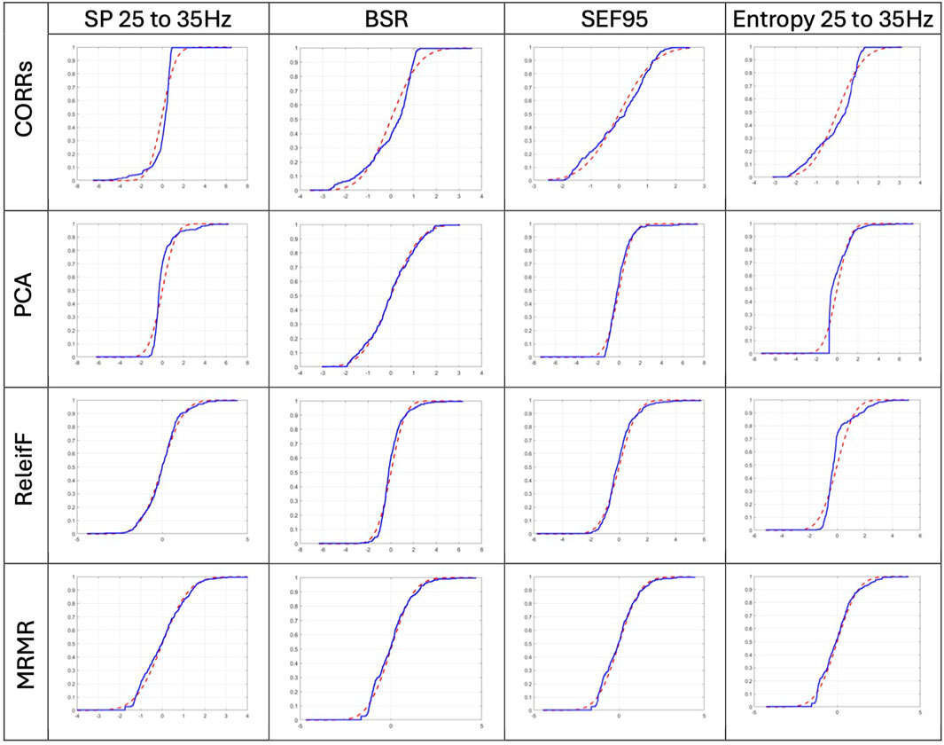
Figure 1. Visual comparison of the selected score vector CDF, blue line, with standard normal CDF with 0 mean and standard deviation 1, red dashed line. Selected score vectors are produced by CORRs, PCA, ReliefF, and MRMR algorithms for BSR, SEF95, SP 25–35 Hz, and entropy 25–35 Hz features, respectively.

The score vectors of best evaluated features have passed the K-S test, while the features that received lower scores, such as Entropy 25–35 Hz, did not. Even visual evaluation of distribution normality of Entropy 25–35 Hz features on Figure 1 has the least normal distribution; this is expected since it was evaluated as the least relevant feature. If one compares the distribution of evaluated scores by CORRs and ReliefF algorithm, ReliefF score vectors better resemble the standard normal CDF than those of CORRs. This corroborates the results of the ReliefF algorithm compared to the CORRs since it is expected that if the evaluation of feature relevance is correct, the answer must be similar among all experiments and, therefore, must be normally distributed with the mean values as the most expected evaluation result.

The results of CORRp and CORRs correlations were very similar to each other, suggesting that EEG features are largely linearly correlated with the reference DoA signal. Therefore, in this paper, we only present the results of CORRs in Figure 2, 7, and 8, as it may also capture more general, non-linear correlations. The distribution of score values for all features evaluation by CORRs correlation, PCA, ReliefF, and MRMR algorithms are presented in Figures 2–6 using a box-and-whisker diagram for each feature.

Figure 2

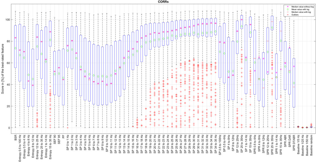
Figure 2. Distribution of Spearman’s coefficient for each evaluated EEG feature.

Figure 3

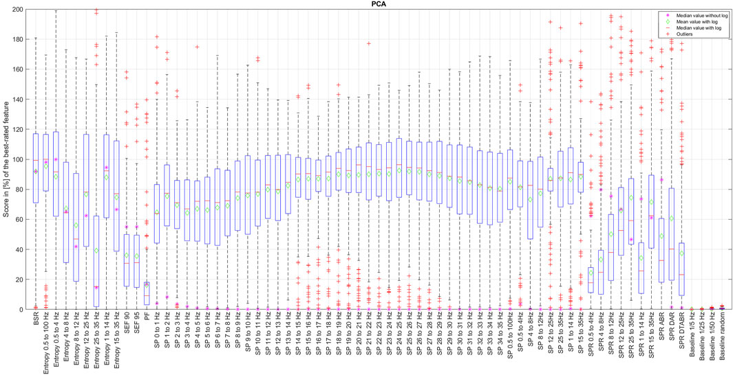
Figure 3. Distribution of the PCA coefficient for each evaluated EEG feature.

Figure 4

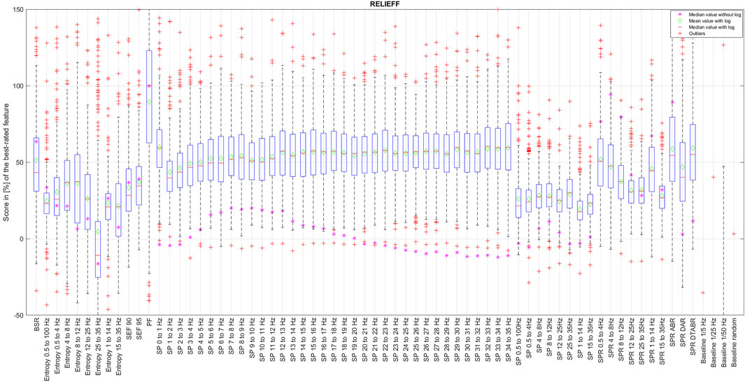
Figure 4. Distribution of the ReliefF coefficient for each evaluated EEG feature.

Figure 5

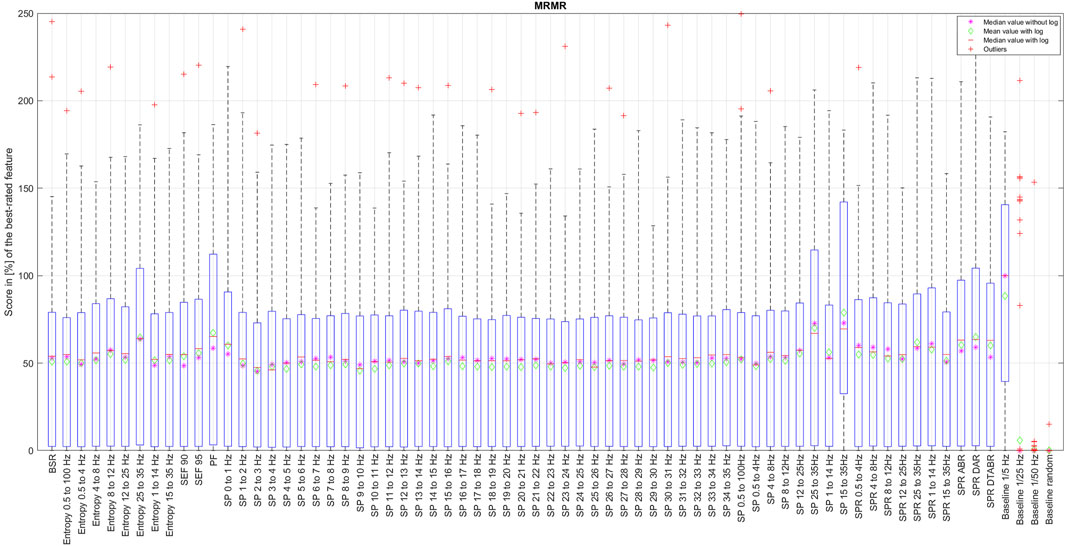
Figure 5. Distribution of the coefficient for each EEG feature ranked by the mRMR algorithm running over the data with a full resolution.

Figure 6

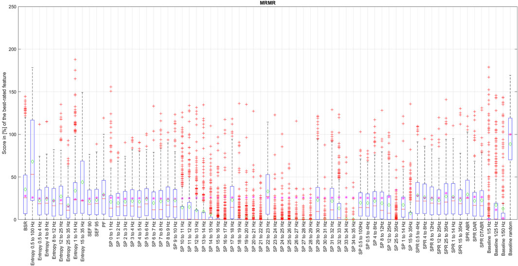
Figure 6. Distribution of the coefficient for each EEG feature ranked by the mRMR algorithm over the data with 1% resolution.

The box in such a representation represents the interquartile range (IQR) between lower Q₁ (0.25) and higher Q₃ (0.75) quartiles, thus covering 50% of the values. The upper (lower) whisker will have a maximum length of 1.5 of IRQ drawn up (down) from the Q₃ (Q₁) quantile. The red crosses indicate the farthest outliers. The mean value is marked with a green diamond while a median value is represented with a small horizontal bar of red color. All scores for SP features are represented in 10log₁₀ scale. However, to compare the score evaluation results of SP features in non-logarithmic scale, we also provide median values of those feature’s scores as a violet asterisk on each graph.

It is also notable that, as expected, all graphs representing score distributions (e.g., Figures 2–6) show that the four baseline signals received very low scores, indicating their non-relevance to DoA. This underscores the appropriateness of evaluating other signals.

3.2 Final score computation

The complete set of feature rankings, along with their scores normalized with the maximum score value from each set defined by one algorithm (CORRs, PCA, and ReliefF) as well as their average score, can be accessed online via¹. The rankings are presented visually in Figure 7. We excluded the evaluation of feature rankings using mRMR as it employs a different principle for ranking, considering not only feature relevance but also reducing information redundancy. Nevertheless, the results of the mRMR feature are depicted in Figures 5 and 6 and discussed further in Section 3.3.

Figure 7

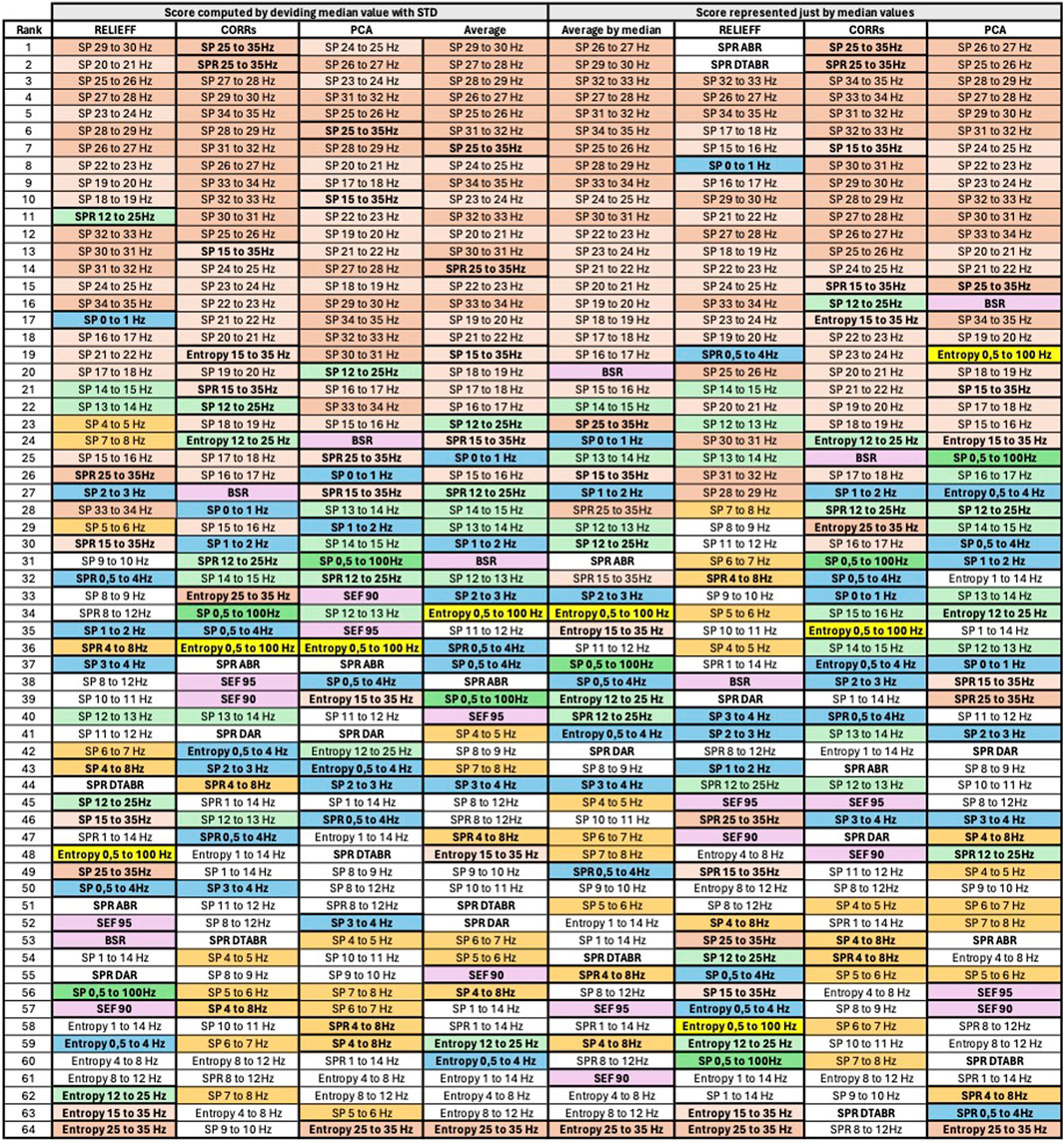
Figure 7. Final features ranking by each algorithm. Left side presents feature ranking based on the formula presented in Section 3.2, while the right side based on median score values sorted in descending order from up to down. To help the reader, we have used similar colors to group SP features based on their frequency. SP features representing frequency ranges larger than 1 Hz are additionally highlighted in bold font. Some other unique features are regrouped with similar color codes, such as BSR, SEF90, and SEF95.

Here are some intuitive rules that we believe are relevant while evaluating the coefficients using the distribution representation.

• Higher values of mean and median correspond to generally higher scores that can be given to the feature.

• If the mean and median values are different, then the distribution is skewed toward the median value, such that on the side of the mean value we have some outliers, values that are very different from the majority of the data.

• A smaller rectangle indicates smaller variability among the values and therefore higher confidence in the mean value of the coefficient.

• If the score given to the baseline signals is low, then the algorithm performed a correct evaluation of the features. The only algorithm where the baseline signal may legitimately receive a high score is mRMR since it will also give higher scores to the features carrying new non-redundant information.

Consequently, different scores unifying formulas can be derived. Here, we present the results of final score evaluation based on the following most obvious formula:

$X_{\mathit{alg}}^{j/total}=\frac{\theta \cdot {\tilde{X}}_{\mathit{alg}}^j\left(exp\right)}{ϵ\cdot IRQ\left(X_{\mathit{alg}}^j\left(exp\right)\right)},$

where $X_{\mathit{alg}}^{j/total}$ is the final unified score for feature j for a selected algorithm alg, ${\tilde{X}}_{\mathit{alg}}^j(exp)$ and $IRQ(X_{\mathit{alg}}^j(exp))$ are the median and the IRQ for scores for feature j among all experiments; θ and ϵ are the parametrization coefficients, allowing change of the relative importance of median and standard deviation scores.

3.3 Analysis of score distributions

There has also been some significant disagreement among algorithms, albeit only regarding one feature from the extensive list: peak frequency (PF). The ReliefF algorithm assigned a very high score to PF, while correlations and PCA did not consider it important at all. We believe that PF values in this evaluation set have low credibility since they do not provide enough resolution to yield reasonable results. Often, the values of PF range from 0 to 1 Hz, as the maximum signal power is at low frequencies. Although we increased the granularity of the PF values to 0.25 Hz, this is still insufficient, judging from the scores given by most algorithms, as a significant portion of the PF values equals 0. Therefore, we have excluded this feature from the analysis presented in this paper. However, we do not rule out the possibility that with improved resolution these features may receive more consistent score evaluations and have the potential to be included in the list of most important features.

Among all the methods that we have examined, mRMR algorithm is the only one that selects features based on their mutual information at the same time, aiming to reduce information redundancy. Since the probabilities p(x), p(y), and p (x, y) of the mRMR algorithm are based on counts of variable X and Z equal to exact values x and z simultaneously, it is clear that the resolution of numerical data will have an essential influence on the result, since resolution here can be seen as a size of the bin of an histogram that should be neither too big nor too small in order to see a correct probability distribution. We have thus applied the mRMR algorithm first to the data with the full resolution, such as bin size too small (see Figure 5), and then, since all numerical values of time-series are normalized, we have run this algorithm with a resolution of 0.01, equivalent to 1% (see Figure 6). This resolution was chosen since the DoA index is usually represented with values between 0% and 100%.

An evaluation of features with mRMR algorithm with different granularity of the data has shown that SP over 14 Hz have low importance, with some exceptions like SP 17–18 Hz and SP 22–23 Hz. This is because, once we round the values down to a maximum of their second decimal, we drastically reduce the data variability in small numbers. This has raised an important observation: data resolution plays an essential role not only in feature importance but generally in algorithm performance. It is also probable that SP of higher frequencies have never been considered since their values are so small that, when they are visualized on a classical density spectral array, it is difficult to notice their correlation with DoA. Having features with such small values naturally leads to the question of how reliable those features would be in a real setting in the presence of electrical noise that can easily alternate their values, leading to an unpredictable impact on DoA estimation.

We have observed a slight difference in feature selection results depending on the data normalization method, such as min-max normalized vs. Z-normalization. For example, some neighboring features could swap their ranking positions. However, if sets of best features, like best-10 or best-20 were selected, those sets would be identical.

Figure 7 presents the visualized ranking of final feature scores for ReliefF, CORRs, and PCA algorithms over z-normalized data. In this table, columns 2–5 represent the scores computed using the formula presented in Section 3.2 with θ and ϵ equal to 1, and columns 6–9 represent ranking of features based only on their median values. All features are sorted in descending order from up to down based on their score.

To assist the reader in following our feature evaluation, we have implemented color coding for features. First, we have used similar colors to group SP features based on their frequency. SP features representing frequency ranges larger than 1 Hz are additionally highlighted in bold font. Moreover, some other unique features are regrouped with similar color codes, such as BSR, SEF90, and SEF95.

3.4 Ranking of best features for DoA estimation

Thanks to the visualization of Figure 7, it can be observed that SP of the signal for frequencies above 14Hz has similarly higher correlation with DoA, evaluated by all algorithms, compared to the SP of signals with frequencies below 14Hz. The spectral power of the frequency bands above 14Hz per se has not been mentioned as essential in the literature. However, Ra et al. (2021) showed that spectral entropy from the 21.5 to 38.5 Hz frequency bands show the highest correlation with BIS, indicating that SP of higher frequencies could have a high potential in DoA estimation.

If we examine features in the temporal domain, such as BSR and Entropy, we observe that BSR exhibits a strong correlation with DoA, a well-established phenomenon in EEG signal processing for anesthesia. Entropy has also attracted significant attention in DoA evaluation. The entropy calculated over a specific component of the time-domain signal, representing the Ψ frequency range (e.g., 15–35 Hz), appears to be a more robust predictor than just the η band (e.g., 25–35 Hz), as demonstrated by three algorithms. However, these results may not be directly comparable to the present study because entropy was here calculated in the time-domain, measuring signal amplitude in [V], while Ra et al. (2021) investigated spectral entropy (SE), which measures entropy over the squared signal amplitude in [V²]. Nevertheless, based on our evaluation, Entropy 0.5–100 Hz exhibits the highest correlation with DoA, followed by Entropy 15–35 Hz. Conversely, Entropy over lower frequencies and narrower bands, such as Entropy 4–8 Hz or Entropy 8 Hz–12 Hz, demonstrates lower importance among all evaluated features.

3.5 Strategies for feature selection

As explained in Section 3.1, selecting the most relevant features using the mRMR algorithm would not be conclusive in our case, as all features are derivatives of the same EEG signal and to some extend carry similar information. Therefore, to summarize the results of this paper, we have devised two strategies for selecting the best features for DoA estimation.

3.6 Strategy 1

If we examine Figure 7, we notice that SP features with higher frequencies within the 1 Hz range (e.g., SP 29–30 Hz or SP 31–32 Hz) are ranked higher than SP features covering larger frequency ranges (e.g., SP 25–35 Hz or SP 15–35 Hz). However, the ranking changes for lower frequencies. For instance, SP 12–25 Hz is ranked higher than SP 14–15 Hz, SP 13–14 Hz, and so forth. Consequently, to reduce information redundancy, for frequencies above 15 Hz one might choose SP features with a 1 Hz range and exclude SP and SPR features with larger ranges. Conversely, for lower frequencies, it may be preferable to retain SP and SPR features with larger ranges and exclude those with a 1 Hz range. An exception among lower-frequency SP features might be made for SP 0–1 Hz, SP 1–2 Hz, SP 2–3 Hz, and SP 3–4 Hz, since three of them are ranked higher than SP and SPR 0.5–4 Hz. The results of feature pruning following this strategy applied to averaged scores computed based on the formula in Section 3.2 (column 5 of Figure 7) are presented in columns 2 and 3 of Figure 8.

Figure 8

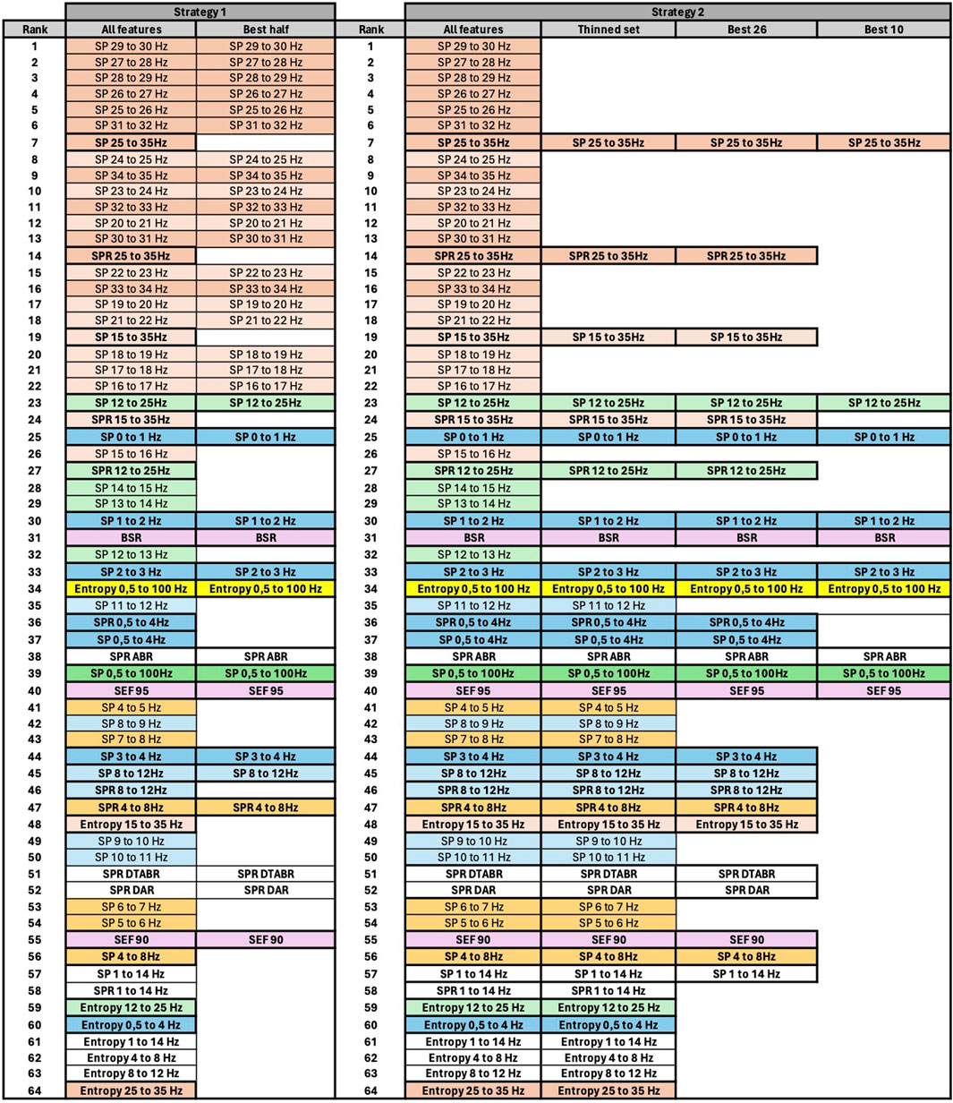
Figure 8. Feature pruning following the two presented strategies.

3.7 Strategy 2

However, considering the crucial observation in Section 3.3 that data resolution may significantly impact prediction stability, one might, when selecting the SP features, prioritize SP features over spectral bands larger than 1 Hz, especially for frequencies above 14 Hz. We may include SP features over narrow frequency bands only for frequencies between 0 and 4 Hz, as they exhibit maximum spectral power. As illustrated in Figure 8, we first prune the SP features for frequencies above 12 Hz. It is noteworthy that SP 15–35 Hz encompasses information of both “SP 25–35 Hz” and “SP 12–25 Hz” features. Additionally, SP and SPR features over the same frequency band are likely to convey similar information, as SPR can be considered a normalized SP signal. Following this rationale, we further select the best 26 and best 10 features. The visualization of each phase of feature pruning is summarized in columns 5–8, Figure 8.

4 Discussion

Application of ML/DL methods for the selection of best features, regardless of the domain of application, has been described previously, and there exists a large list of methods that can be applied. A comprehensive review of feature selection methods has been presented by Theng and Bhoyar (2024). Both general methods and more specific applications have been reported. General methods are as various as principal component analysis (PCA), linear discriminant analysis (LDA), mutual information-based, correlation-based, wrapper-based, embedded, multi-objective, fuzzy, evolutionary, random probes-based, and evaluation measure. The most promising techniques from this list have been included in the present investigation—PCA, mutual information-based, correlation-based, and embedded—and have been applied to a specific case study of EEG signal features.

Similar to the approach presented in this paper, Anand et al. (2023) applied feature selection specifically on EEG signals for the purpose of DoA estimation. However, they extracted features only in the time domain and used only one feature selection method—a tree classifier. They then trained multiple DoA classifier methods using selected features and concluded that random forest had the best performance among chosen algorithms. Such a conclusion is expected since features were selected by an embedded method based on a tree classifier. There are also many studies which have focused on evaluating specific EEG features as predictors of DoA. For example, entropy has received much attention, being examined for ability to estimate the DoA.

In human anesthesia, it is known that different parts of the brain may provide distinct EEG signatures, thus carrying different information in response to general anesthesia (Yeom et al., 2017). The PSI index, for example, accounts for changes in symmetry and synchronizations between brain regions and the inhibition of frontal cortex regions (Drover and Ortega, 2006). Special attention has also been given to phase lag entropy (Shin et al., 2020; Jun et al., 2019; Kim et al., 2021), a measurement of temporal pattern diversity in the phase relationship between two EEG signals from prefrontal and frontal montages. This study worked with veterinary data, and the difference in EEG signal between prefrontal and frontal montages was less pronounced. We have not therefore differentiated between signal collected from different scalp locations and thus have evaluated the entropy of each collected EEG signal separately. Moreover, we compute entropy over temporal domain EEG signal, even though in some research spectral entropy (SE) correlated with BIS (Ra et al., 2021) has been investigated. The biggest difference in the two approaches to entropy computation is that the SE is computed over the squared amplitude values of the temporal domain. The main reason for choosing the entropy of the temporal domain over the SE is in the goal of implementing DoA estimation in real-time where one entropy value would be expected every 1s. This is clearly possible when entropy is computed, for example, over 200 samples of EEG signal (200 Hz sampling rate). In the case of SE, the time-frequency conversion of the EEG signal first occurs, which in turn would reduce the number of SP values per second and only after SE can be calculated, which risks providing values only every several seconds.

All these studies evaluate the importance of only one feature, such as different types of entropy, while the importance of other features/predictors in parallel is not investigated. Like Anand et al. (2023), this paper investigates the relative importance of EEG features by evaluating a larger set of features from both time and frequency domains while evaluation is performed by a larger set of selection algorithms.

The results presented here must be interpreted against the limitations of the methodology. As all EEG signals from bilateral acquisition and from the placement of different electrodes on the skull have been included, the proposed feature selection is global and not specific for a particular electrode setting. Similar information may have been carried by EEG signals reported from close electrodes recording EEG activity in the same animal, potentially leading to data duplication. However, this is not expected to impact feature selection and may allow confirmation of feature relevance over signals of various amplitudes and noise contamination. The use of a PK-PD-derived predicted effect curve based on the information from propofol delivery rates as a reference signal for supervised algorithms can be questioned. Most publications applied BIS measurements for this purpose. Although this was not available for the pigs in the present investigation, BIS values are not validated in pigs. Moreover, it was the authors’ intention to use a reference signal not essentially based on EEG to avoid the paradox of selecting EEG features referenced by their own signal. There is no recognized gold standard for using genuine values as a reference for DoA, and the PKPD approach presented here was considered a fair attempt, given its own limitations.

5 Conclusion

In this paper, we presented an approach for measuring the prediction capability of EEG features for DoA estimation in pigs. The results of feature evaluation, conducted with essentially four algorithms, were presented along with two strategies for pruning the feature set. These algorithms (correlation, PCA, ReliefF, and mRMR) include variance computation in their core. The choice of algorithms in this paper was driven by the idea of linking upcoming results with the established practice of DoA estimation using BIS and PSI, where formulas for DoA estimation are arithmetic combinations of features with higher correlation with DoA.

However, we also evaluated other algorithms such as Random Forest and L1/L2 regularization, which have a loss function at their core. They presented slightly different rankings for the same set of features. For example, they ranked lower the SP of frequencies between 8 and 25 Hz, although they were consistent with the presented algorithms regarding SP of frequencies higher than 25 Hz as well as lower than 8 Hz. It is also clear that the choice of feature selection algorithm must take into account the algorithm planned for use with the DoA estimation. However, the results of this paper should be seen as a first step toward selecting the best performing machine learning/ deep learning algorithm for DoA estimation.

Data availability statement

The original contributions presented in the study are included in the article/supplementary material; further inquiries can be directed to the corresponding author.

Author contributions

BC: software, visualization, writing–review and editing, and writing–original draft. GM: formal analysis, supervision, writing–review and editing, and writing–original draft. AM: conceptualization, validation, writing–review and editing, and writing–original draft. OL: conceptualization, supervision, validation, writing–review and editing, and writing–original draft. AS: conceptualization, data curation, formal analysis, funding acquisition, investigation, methodology, project administration, resources, supervision, validation, visualization, writing–original draft, and writing–review and editing.

Funding

The author(s) declare that financial support was received for the research, authorship, and/or publication of this article. This article was funded by “Jeunes chercheurs” HES-SO funding in 2022–2024.

Conflict of interest

The authors declare that the research was conducted in the absence of any commercial or financial relationships that could be construed as a potential conflict of interest.

Publisher’s note

All claims expressed in this article are solely those of the authors and do not necessarily represent those of their affiliated organizations, or those of the publisher, the editors, and the reviewers. Any product that may be evaluated in this article, or claim that may be made by its manufacturer, is not guaranteed or endorsed by the publisher.

Footnotes

¹https://gitlab.hevs.ch/alena.simalats/rt-doai-vet/- /blob/main/Features Selection.xlsx

References

Afshar, S., Boostani, R., and Sanei, S. (2021). A combinatorial deep learning structure for precise depth of anesthesia estimation from EEG signals. IEEE J. Biomed. Health Inf. 25, 3408–3415. doi:10.1109/JBHI.2021.3068481

CrossRef Full Text | Google Scholar

Anand, R. V., Abbod, M. F., Fan, S.-Z., and Shieh, J.-S. (2023). Depth analysis of anesthesia using eeg signals via time series feature extraction and machine learning. Sci 5, 19. doi:10.3390/sci5020019

CrossRef Full Text | Google Scholar

BIOPAC Systems Inc (2023). BIOPAC MP160 EEG acquisition device. Available at: https://www.biopac.com/.

Google Scholar

Bustomi, A., Wijaya, S. K., and Prawito, S. (2017). Analyzing power spectral of electroencephalogram (eeg) signal to identify motoric arm movement using emotiv epoc+. AIP Conf. Proc. doi:10.1063/1.4991175

CrossRef Full Text | Google Scholar

Connor, C. (2022). Open reimplementation of the bis algorithms for depth of anesthesia. Anesth. Analgesia 135, 855–864. doi:10.1213/ane.0000000000006119

CrossRef Full Text | Google Scholar

Drover, D., and Ortega, H. R. (2006). Patient state index. Best Pract. Res. Clin. Anaesthesiol. 20, 121–128. doi:10.1016/j.bpa.2005.07.008

PubMed Abstract | CrossRef Full Text | Google Scholar

Egan, T., Kern, S., Johnson, K., and Pace, N. (2003). The pharmacokinetics and pharmacodynamics of propofol in a modified cyclodextrin formulation (captisol) versus propofol in a lipid formulation (diprivan): an electroencephalographic and hemodynamic study in a porcine model. Anesth. analgesia 97, 72–79. doi:10.1213/01.ane.0000066019.42467.7a

PubMed Abstract | CrossRef Full Text | Google Scholar

Eleveld, D., Colin, P., Absalom, A., and Struys, M. (2018). Pharmacokinetic–pharmacodynamic model for propofol for broad application in anaesthesia and sedation. Br. J. Anaesth. 120, 942–959. doi:10.1016/j.bja.2018.01.018

PubMed Abstract | CrossRef Full Text | Google Scholar

Fahy, B., and Chau, D. (2018). The technology of processed electroencephalogram monitoring devices for assessment of depth of anesthesia. Anesth. Analgesia 126, 111–117. doi:10.1213/ANE.0000000000002331

CrossRef Full Text | Google Scholar

Hochreiter, S., and Schmidhuber, J. (1997). Long short-term memory. Neural Comput. 9, 1735–1780. doi:10.1162/neco.1997.9.8.1735

PubMed Abstract | CrossRef Full Text | Google Scholar

Hwang, E., Park, H.-S., Kim, H., Kim, J.-Y., Jeong, H., Kim, J., et al. (2023). Development of a bispectral index score prediction model based on an interpretable deep learning algorithm. Artif. Intell. Med. 143, 102569. doi:10.1016/j.artmed.2023.102569

PubMed Abstract | CrossRef Full Text | Google Scholar

Johansen, J. W. (2006). Update on bispectral index monitoring. Best Pract. Res. Clin. Anaesthesiol. 20, 81–99. doi:10.1016/j.bpa.2005.08.004

PubMed Abstract | CrossRef Full Text | Google Scholar

Jolliffe, I., and Cadima, J. (2016). Principal component analysis: a review and recent developments. Philosophical Trans. R. Soc. A Math. Phys. Eng. Sci. 374, 20150202. doi:10.1098/rsta.2015.0202

PubMed Abstract | CrossRef Full Text | Google Scholar

Jun, M., Yoo, J., Park, S., Na, S., Kwon, H., Nho, J., et al. (2019). Assessment of phase-lag entropy, a new measure of electroencephalographic signals, for propofol-induced sedation. Korean J. Anesthesiol. 72, 351–356. doi:10.4097/kja.d.19.00019

PubMed Abstract | CrossRef Full Text | Google Scholar

Kim, K.-M., Lee, K.-H., and Park, J.-H. (2021). Phase lag entropy as a surrogate measurement of hypnotic depth during sevoflurane anesthesia. Medicina 57, 1034. doi:10.3390/medicina57101034

PubMed Abstract | CrossRef Full Text | Google Scholar

Kreuer, S., and Wilhelm, W. (2006). The narcotrend monitor. Best Pract. Res. Clin. Anaesthesiol. 20, 111–119. doi:10.1016/j.bpa.2005.08.010

PubMed Abstract | CrossRef Full Text | Google Scholar

Lee, H., Ryu, H., Park, Y., Yoon, S., Yang, S., Oh, H., et al. (2019). Data driven investigation of bispectral index algorithm. Sci. Rep. 9, 13769. doi:10.1038/s41598-019-50391-x

PubMed Abstract | CrossRef Full Text | Google Scholar

Lobo, F., and Schraag, S. (2011). Limitations of anaesthesia depth monitoring. Curr. Opin. Anaesthesiol. 24, 657–664. doi:10.1097/ACO.0b013e32834c7aba

PubMed Abstract | CrossRef Full Text | Google Scholar

Long, F., Peng, H., and Ding, C. (2005). Feature selection based on mutual information: criteria of max-dependency, max-relevance, and min-redundancy. IEEE Trans. Pattern Analysis Mach. Intell. 27, 1226–1238. doi:10.1109/TPAMI.2005.159

PubMed Abstract | CrossRef Full Text | Google Scholar

Mirra, A., Gamez Maidanskaia, E., Levionnois, O., and Spadavecchia, C. (2024a). How is the nociceptive withdrawal reflex influenced by increasing doses of propofol in pigs? Animals 14, 1081. doi:10.3390/ani14071081

PubMed Abstract | CrossRef Full Text | Google Scholar

Mirra, A., Micieli, F., Arnold, M., Spadavecchia, C., and Levionnois, O. (2024b). The effect of methylphenidate on anaesthesia recovery: an experimental study in pigs. PLoS One 19, e0302166. doi:10.1371/journal.pone.0302166

PubMed Abstract | CrossRef Full Text | Google Scholar

Mirra, A., Spadavecchia, C., and Levionnois, O. (2022a). Correlation of sedline-generated variables and clinical signs with anaesthetic depth in experimental pigs receiving propofol. PLoS One 17, e0275484. doi:10.1371/journal.pone.0275484

PubMed Abstract | CrossRef Full Text | Google Scholar

Mirra, A., Spadavecchia, C., and Levionnois, O. (2022b). Correlation of sedline-generated variables and clinical signs with anaesthetic depth in experimental pigs receiving propofol. PLOS ONE 17, 02754844–e275512. doi:10.1371/journal.pone.0275484

CrossRef Full Text | Google Scholar

Purdon, P., Sampson, A., Pavone, K., and Brown, E. (2015). Clinical electroencephalography for anesthesiologists. Anesthesiology 123, 937–960. doi:10.1097/aln.0000000000000841

PubMed Abstract | CrossRef Full Text | Google Scholar

Ra, J. S., Li, T., and Li, Y. (2021). A novel spectral entropy-based index for assessing the depth of anaesthesia. Brain Inf. 8, 10. doi:10.1186/s40708-021-00130-8

CrossRef Full Text | Google Scholar

Robnik-Šikonja, M., and Kononenko, I. (2003). Theoretical and empirical analysis of relieff and rrelieff (article). Mach. Learn. 53, 23–69. doi:10.1023/a:1025667309714

CrossRef Full Text | Google Scholar

Saby, J. N., and Marshall, P. J. (2012). The utility of eeg band power analysis in the study of infancy and early childhood. Dev. Neuropsychol. 37, 253–273. doi:10.1080/87565641.2011.614663

PubMed Abstract | CrossRef Full Text | Google Scholar

Schmierer, T., Li, T., and Li, Y. (2024). Harnessing machine learning for EEG signal analysis: innovations in depth of anaesthesia assessment. Artif. Intell. Med. 151, 102869. doi:10.1016/j.artmed.2024.102869

PubMed Abstract | CrossRef Full Text | Google Scholar

Shin, H., Kim, H., Jang, Y., You, H., Huh, H., Choi, Y., et al. (2020). Monitoring of anesthetic depth and eeg band power using phase lag entropy during propofol anesthesia. BMC Anesthesiol. 20, 49. doi:10.1186/s12871-020-00964-5

PubMed Abstract | CrossRef Full Text | Google Scholar

Theng, D., and Bhoyar, K. K. (2024). Feature selection techniques for machine learning: a survey of more than two decades of research. Knowl. Inf. Syst. 66, 1575–1637. doi:10.1007/s10115-023-02010-5

CrossRef Full Text | Google Scholar

Yeom, S., Won, D., Chi, S., Seo, K., Kim, H., Müller, K., et al. (2017). Spatio-temporal dynamics of multimodal eeg-fnirs signals in the loss and recovery of consciousness under sedation using midazolam and propofol. PLoS One 12, e0187743. doi:10.1371/journal.pone.0187743

PubMed Abstract | CrossRef Full Text | Google Scholar