Evaluation of different erosion models for predicting guide vane wear in Francis turbine

Guide vanes (GVs) are one of the components of the Francis turbine that are most vulnerable to erosion. Presence of hard minerals including feldspar and quartz cause erosion on the surface of GVs. This results in damage and disturbances in the functioning of the turbine. Computational Fluid Dynamics (CFD) methods are useful to estimate erosion but are dependent significantly on erosion models used for simulations. A three guide vane cascade (3GV) rig is a simplified setup that recreates the flow around GVs. Previous studies have used the setup to visualize the secondary flows around the GVs using Particle Image Velocimetry (PIV) and CFD techniques that could be one of the major causes of erosion in Francis turbine. In this study, an Eulerian-Lagrangian approach with Reynolds Averaged Navier Stokes (RANS) based Shear Stress Transport (SST) turbulence model has been used to develop a numerical model of the same rig. The erosion caused by the sediment-laden flow has been quantified and visualized by employing Finnie, Nandakumar, Oka, and Tabakoff and Grant erosion models. This study has been conducted to determine which of the erosion model predicts the erosion pattern closer to the real case of eroded GV of Jhimruk Hydro-Electric Plant (HEP). The focus of the study is the clearance gap (CG) of the GV. By dividing the CG into sections and comparing the erosion predictions by different erosion models with the actual erosion, Finnie erosion model is found to be the most suitable model for this application. The severity and area affected due to erosion as predicted by this model is found to most closely match the erosion observed in the CG of the real hydropower plant’s GV, specially at three different locations: trailing edge of suction side (SS-TE), leading edge of suction side (SS-LE) and the middle of the leading edge (MS-LE).

1 Introduction

Sediment erosion in hydraulic turbines has been a major problem across the world especially in the hydropower located in the regions with steep terrain and young topography like the Himalayas, Andes, Alps and the Pacific ranges (Winkler, 2014). Sediments consist of hard minerals such as quartz and feldspar which erode various hydropower components, especially the turbine components (Kapali et al., 2019). In turbines, the factors affecting erosion include flow phenomena, shape of the eroded surfaces, properties of the materials, applied force and pressure by the sediments, properties of the sediments and the relative speeds at which they interact (Burwell, 1957; Thapa, 2004a). This is a broad interpretation of erosion in turbines, but as the flow in turbines is complicated, the erosion phenomena largely depend upon the flow. The flow of the water in turbines varies with the working principle of the turbine, whether it is an impulse turbine like Pelton turbine, or a reaction turbine like Francis or Kaplan turbine. The flow may vary within the same turbine or a component of the turbine. Hence, it is important to analyze the flow phenomena in a turbine to understand the way erosion takes place and plan to optimize the turbine so that the turbine gets less affected by erosion. Francis turbine is a mixed-flow reaction turbine with radial and axial water flow within the runner (Bansal, 2010). Francis turbine’s most affected components due to erosion are the face plates, GVs, stay vanes, and runner blades (Noon and Kim, 2021). GVs guide the flow entering the runner and control the flow according to the operating conditions required. They are typically made to the shape of a hydrofoil which maintains a pressure difference across its two sides. This is essential to accelerate the flow and convert the energy of the water to kinetic energy (Koirala et al., 2017). When two solid bodies in relative motion are in contact with each other, friction and wear occur (Stojanovic and Ivanovic, 2014). To prevent such wear and to perform its function correctly, a small clearance is added between the GV surface and the upper side and lower side housing. The pressure difference between the two sides of the vane forces water to flow from the higher-pressure zone to lower pressure zone through the CG. As the cascade itself is at a higher pressure than the environment, it expands the CG. Further, due to presence of sediment particles, the flow that occurred because of the pressure difference between two sides can erode the upper and lower surface and the GV surface facing them. Hence, CG can increase from the nominal value required for the movement of GVs. This would allow for greater flow across the gap, which further causes erosion. This flow, termed as leakage flow, disturbs the primary flow that was optimized for the runner at that operating condition. Further, past researchers have identified it as one of the causes of erosion at the leading edge of the runner (Chitrakar, 2018).

In addition to the erosion due to leakage flow, GVs are subjected to other types of erosion mechanism. There are four different types of erosion that can occur in the GVs: turbulence erosion, secondary flow erosion, leakage flow erosion, and acceleration erosion. Turbulence erosion occurs when there is a high velocity of fine particles at the GV outlet, secondary flow erosion occurs when there is a horseshoe vortex caused by secondary flow from the clearance gap, leakage flow erosion occurs due to the leakage flow caused due to the pressure difference at the CG of the GV, and acceleration erosion occurs when there is a high velocity of coarse particles at the CG (Chitrakar et al., 2016; Chitrakar et al., 2018a; Kumar Sahu and Kumar Gandhi, 2022). Figure 1 illustrates the erosion in the Francis turbine GV, particularly the leakage erosion at the face plate and CG.

Figure 1

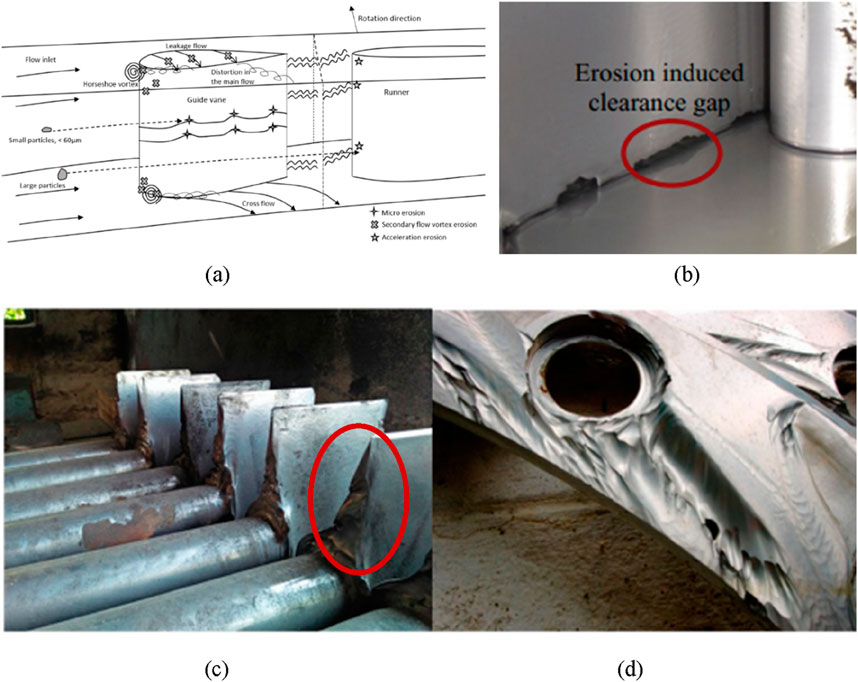
Figure 1. Francis turbine guide vane (A) Erosion phenomena due to different flows (Chitrakar et al., 2016) (B, C) erosion due to leakage flows at GV (Chitrakar et al., 2018b; Koirala et al., 2019) (D) erosion due to leakage flows at the facing plate (Chitrakar et al., 2018b).

1.1 Three guide vane cascade rig

The three Guide Vane (3GV) cascade rig is a research setup with three simplified GVs organized in a cascade configuration. This setup is used for conducting experiments and numerical simulation to investigate the leakage flow within the GVs. The 3GV cascade setup is used to examine the flow around the GV. The setup was developed using the design approach outlined by Thapa et al. (2016). This configuration is effective in minimizing the wall effects on the flow region around the central GV. The walls of the test setup were designed using theory of free vortices. The main goal of this setup is to replicate the velocity components, ensuring flow similarity with the model turbine, although the influence of rotating runner vanes on the GVs is disregarded and instead of round curvature of spiral casing, plates that provide the required radial and tangential velocity are kept. The development of the 3GV cascade rig from Francis turbine GV is shown in Figure 2.

Figure 2

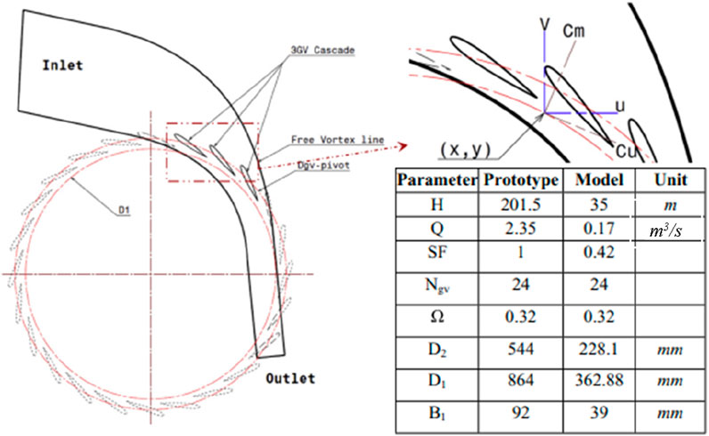
Figure 2. Development of 3GV cascade rig (Koirala et al., 2019).

The tangential and meridional velocity components, C_u and C_m, were analogous to those in a real turbine. The C_u component contributed to the work done and power generation, while the C_m component controlled the direction of the downstream flow. The equation for C_u and C_m is given in Equations 1, 2.

$C_m=-\left(u.\cos \theta +v.\sin \theta \right)(1)$

$C_u=\left(u.\sin \theta -v.\cos \theta \right)(2)$

Thapa conducted (Thapa et al., 2016) a numerical analysis to investigate the leakage flow in 3GV and single GV cascade rig and developed an experiment setup of single GV cascade rig taking the data from the Jhimruk HEP as reference to study about the velocity components of the turbine. Chitrakar et al. (2017), Chitrakar et al. (2019a) developed and used 3GV cascade rig to investigate the leakage flow from the CG of GV using Particle Image Velocimetry (PIV) for different GV angles and different GV profiles. Koirala et al. (2019) used 3GV cascade rig to observe the erosion patterns in GV at a concentration of 1,300 ppm. The present study expands the previous research done on understanding the leakage flow in 3GV cascade rig by modelling the flow dynamics and sediments behavior in 3GV cascade rig numerically using an open-source CFD software, OpenFOAM. The results hence obtained present the locations where the GVs are susceptible to erosion. Comparison of different erosion models are applied in the study to determine which of the used erosion model predicted the erosion pattern closest to the real case. In this study, only the erosion at the clearance gap of the guide vane is considered. This allows for a more comprehensive analysis of erosion phenomena in this system with a complex flow. Figure 3 shows the experimental and 3D model setup of the simplified 3GV cascade rig.

Figure 3

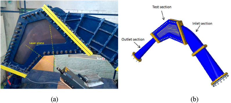
Figure 3. (A) Experimental setup of 3GV cascade rig (B) 3D model of 3GV cascade rig (Chitrakar et al., 2019b).

Various erosion models have been applied to study erosion at different locations of turbo-machineries. Noon and Kim (2021) used Finnie erosion model to predict the erosion at different components of Francis turbine as this model uses combination of the Lagrangian method for particle tracking and Eulerian multiphase techniques. Acharya et al. (2019) performed a numerical simulation of the Francis turbine aimed at assessing the erosion rate density of the NACA0012 GV profile at the best efficiency point (BEP) using the Tabakoff and Grant erosion model along with the SST k-omega turbulence model. Rakibuzzaman et al. (2019) also used Tabakoff and Grant erosion model to calculate erosion rate density in the Francis Turbine. López et al. (1995) used Nandakumar erosion model to calculate the volume eroded by the impacts of the particles on the material’s surface.

While different numerical studies have been conducted to study the erosion on prone locations in Francis Turbine and GVs, the choice of erosion model has been subjective. A similar study has been conducted for a pump impeller (López et al., 1995). The findings of the current study will help to understand which erosion model will most accurately predict the erosion in the CG.

2 Mathematical model

The governing equation to model the fluid flow is Navier-Stokes equation and continuity equation, while the sediment transport is simulated using a multiphase flow approach. For simulating fluid flow within the 3GV cascade rig and studying erosion, the continuity equation plays a vital role. The continuity equation is a fundamental principle in fluid dynamics that represents the conservation of mass within a fluid domain. It ensures that the mass entering a given region of the flow field is equal to the mass leaving that region, which is crucial for maintaining the physical integrity of the simulation and accurately modelling the flow and sediment transport. This is interpreted as the net change in velocity and net flow of mass across the boundaries is zero (Anderson, 1995). The equations used for this numerical flow analysis follow Reynolds Averaged Navier Stokes (RANS) equation and apply turbulence model based on the eddy viscosity concept (Lenarcic et al., 2015). The governing equations RANS for continuity and momentum are expressed in Equations 3–5.

$\frac{\partial \rho }{\partial t}+\nabla .\left(\rho u\right)=0:\text{Conservation\hspace{0.17em}of\hspace{0.17em}mass}(3)$

Equation 3 states that the rate of change of density (∂ρ/∂t) plus the divergence of the mass flux (∇.(ρu)) equals to zero, which means mass is conserved in the fluid flow. The momentum equation plays an important part for the numerical study on erosion in GVs due to leakage flow in a 3GV cascade rig. In fluid dynamics, the momentum equation is used to describe the motion of fluid and is vital for understanding how forces act on the fluid within the rig. So, this equation is applied in governing fluid flow, fluid interaction with GV, predicting erosion and turbulence modelling. The momentum equation is mathematically expressed as:

$\rho \frac{DV}{Dt}=\rho g+\nabla .{\tau }^{\prime }ij-\nabla p:\text{Conservation\hspace{0.17em}of\hspace{0.17em}momentum}(4)$

$\rho \frac{Dh}{Dt}=\frac{Dp}{Dt}+\nabla \left(k\nabla T\right)+\mathit{\varphi }:\text{Conservation\hspace{0.17em}of\hspace{0.17em}energy}(5)$

Equation 4 states that the rate of change of momentum of a fluid element is balanced by the forces acting on it which are gravitational force, viscous forces, and pressure forces where ρ is the fluid density, DV/Dt represents the fluid acceleration, g is acceleration due to gravity, τ′ is the viscous stress on the fluid and ∇p is the pressure gradient. Equation 5 states that the rate of change of enthalpy is balanced by the work done by pressure forces, heat transfer due to conduction, and viscous dissipation where ρ is the fluid velocity, h is the specific enthalpy of fluid, ∇·(k∇T) is the net rate of heat transfer due to conduction and φ is the viscous dissipation.

2.1 Particle transport model

Sediment transport equations are vital for modelling the movement of sediment particles within the flow, which is important in understanding erosion patterns and predicting the wear and tear on the GVs. Sediment transport equations apply to particle movement which is essential for erosion prediction. Sediment transport equation model could be different according to the nature of the study; if the sediment particles are treated as a separate phase within the fluid and the equations are solved for both the fluid phase and the sediment phase, then the model is Eulerian-Eulerian model and if individual sediment particles are tracked as discrete entities within the fluid flow, then the model is Eulerian-Lagrangian model. In this numerical simulation study, the Eulerian-Lagrangian sediment transport model has been used. The particle transport equation is expressed as in Equation 6.

$F_P=m_p\frac{d{V}_p}{dt}=F_D+F_p+F_g+F_A(6)$

In Equation 6, F_A stands for force of additional mass, F_p for pressure gradient, F_g for buoyancy and gravity and F_D for drag force acting on the particle. In this approach the forces that operate on the particles due to the flow of the carrying medium is calculated to determine the magnitude and direction of velocity of the particles.

2.2 Erosion model

Erosion model is a mathematical relation between quantified value of erosion and the aspects influencing them. Different erosion models are derived from the experiments, observations from real case and numerical analysis on different materials, so some of the influencing factors may vary in different models. Some of the erosion model have also been found to predict the erosion in the turbine. Generally, in hydraulic turbines, the turbine operating conditions, sediment characteristics, properties of materials and velocity of particles are the major influencing factors.

The flow in turbines is complicated where along with the aforementioned factors other criteria also may intervene. The fluid velocity will typically determine the erosion rate; greater velocities lead to increased erosion due to the high particle impact energy of particles. Another consideration is the hardness extent; materials with a higher degree of hardness are likely to exhibit superior erosion resistance. The shape of particle colliding has also been found to impact the severity of the wear in materials, the irregular shape particles caused more severe wear than the round particles (Shrestha et al., 2019). Furthermore, because bigger and more dense particles produce noticeably more wear than smaller ones, particle size and concentration are also crucial. Some of the basic form of erosion model are expressed in Equations 7–11.

Bardal (1985) considered the major factors that affect the wear in turbine and developed a simple erosion model expressed as:

$W=K_{mat}.K_{env}.C.V_p^m\left(\text{mm}/\text{year}\right)(7)$

where, W is the rate of erosion, K_mat is a constant of the material; K_env is constant of the environment; C is the particle concentration; and f(α) is a function of the impingement angle α. The particle’s velocity is denoted by V_p, and its exponent is m.

Using stainless steel as the test material with silica in water as erodent, Tsuguo (1999) derived a more specific erosion model applied for hydro-turbines which is expressed as:

$W=\beta .C^x.a^y.k_1.k_2.k_3.V^m\left(\text{mm}/\text{year}\right)(8)$

where, W represents the thickness loss per unit of time, β the turbine coefficient at the eroded portion, V the relative flow velocity, α the average grain size coefficient, k₁ and k₂ the shape and hardness coefficients of the sand particles, and k₃ the material’s abrasion resistance coefficient.

The IEC standard (IEC, 2009) erosion model to predict the depth of erosion model is expressed as:

$S=W^3.PL.K_m.K_f\left(\text{mm}\right)(9)$

where, S stands for abrasive depth, W for flow velocity, PL for particle load (derived from the integration of particle concentration over time), K_m for material factor, and K_f for flow factor.

Thapa et al. (2012) developed an empirical relationship that could forecast the rate of erosion in the turbine based on his findings for 16Cr5Ni which is the most often used material in turbines. Thapa erosion model is expressed as:

$E=C.K_{hardness}.K_{shape}.K_m.K_f.a.{size}^b\left(\text{mm}/\text{year}\right)(10)$

${\eta }_r={a\left(erosionrate\right)}^b\left[\%/year\right](11)$

where, E and η_r is the erosion rate, k_size, k_shape and k_hardness are the factors that characterizes the relationship between abrasion and the abrasive particle size, shape and hardness, K_m is the component that describes the relationship between the base material’s material properties and abrasion and K_f is the element that best describes the relationship between each component’s water flow and abrasion.

These are some of the early and basic form to forecast the erosion using erosion models in turbines. However, the considered factors are not enough to accurately predict the fluid-particle-material interactions in turbine. Other detailed erosion models have proposed modifications for better erosion estimations and particle behavior. Each model has its own limitations and hence may not be applicable for all studies. In this study, Finnie, Tabakoff and Grant, Nandakumar and Oka Erosion Model are applied in OpenFOAM. The selected models are described in the succeeding sections. The erosion pattern results were normalized with its value to compare the erosion pattern observed between the erosion model. The detail explanation about the process is explained in the topic Methodology.

2.2.1 Finnie Erosion model

Finnie erosion model was derived from the experiments in ductile and brittle materials. The materials’ rate of erosion was studied by solving the motion equations for abrasive particles interacting with the materials’ surface. Finnie erosion model includes three equations; two are for the ductile materials like the materials used in turbine depending upon the angle of attack and the other for the brittle materials. Finnie erosion model accounts for both low angle erosion and the erosion at normal angle (Finnie, 1960). The expression of Finnie erosion model is expressed in Equations 12–14.

Ductile Materials,

$Q=\frac{m{V}^2}{p\psi K}\left(\mathit{sin}2\alpha -\frac{6}{K}{\left(\mathit{sin}\alpha \right)}^2\right)\left({\mathrm{m}}^3\right)if\mathit{tan}\alpha \le \frac{K}{6}(12)$

$Q=\frac{m{V}^2}{p\psi K}\left(\frac{K{\left(\mathit{cos}\alpha \right)}^2}{6}\right)\left({\mathrm{m}}^3\right)if\mathit{tan}\alpha \ge \frac{K}{6}(13)$

Brittle Materials,

$d=\left(constant\right){\left(V\sin \alpha \right)}^{0.4}(14)$

where, Q is the volume of materials eroded, m is the particle grain mass, V is the velocity of the fluid, d is the diameter of the ring crack, p is the shape factor, ψ is the impact angle of the particle relative to the exterior, α is the impingement angle and K is the erosion constant.

2.2.2 Nandakumar erosion model

K. Nandakumar et al. (López et al., 1995) separated erosion into cutting and deformation wear and created an erosion model that forecasts the volume degraded by repeated particle effects on a surface. The expression of Nandakumar erosion model is written in Equation 15.

$\Delta Q=Cm{\rho }_p^{0.15}{\left(V_0\sin \theta \right)}^{2.3}+D{m}^{1.1875}{d}_p^{-0.0625}{V}_0^{2.375}{\left(\cos \theta \right)}^2{\left(\sin \theta \right)}^{0.375}\left({\mathrm{m}}^3\right)(15)$

where C = 7.5*10^–4 and D = 0.082 represent empirical constants, m is the particle’s mass, d_p is its diameter, V₀ is its impact velocity, ρ_p is its density, and θ is its angle of impact.

2.2.3 Tabakoff and Grant erosion model

Tabakoff and Grant (Grant and Tabakoff., 1973) created a model for erosion based on the notion that erosion is dependent on two different mechanisms: one that functions at low angles of attack and the other at high angles of attack. When impacts happen at intermediate approach angles, a combination of the two mechanisms takes place. The equation of Tabakoff and Grant erosion model is expressed in Equations 16–19.

$E=f\left(\gamma \right)\left(\frac{V_P}{V_1}\right){\left(\mathit{cos}\gamma \right)}^2\left[1-R_T^2\right]+f\left(V_{PN}\right)\left(\text{kg}/{\mathrm{m}}^2\right)(16)$

$\begin{array}{c}f\left(\gamma \right)={\left[1+k_2{k}_{12}\mathit{sin}\left(\gamma \frac{\frac{\pi }{2}}{{\gamma }_o}\right)\right]}^2\\ k_2=\left\{1.0if\gamma \le 2{\gamma }_0\right\}\\ k_2=\left\{0.0if\gamma >2{\gamma }_0\right\}\end{array}(17)$

$R_T=1-\frac{v_p}{v_3}\mathit{sin}\gamma (18)$

$f\left(V_{PN}\right)={\left(\frac{v_p}{v_3}\mathit{sin}\gamma \right)}^4\left(\text{kg}/{\mathrm{m}}^2\right)(19)$

where, E is the erosion rate, V_p is the velocity of particles, γ₀ is the angle of maximum erosion, V₁ is the reference velocity 1, V₂ is the reference velocity 2, V₃ is the reference velocity 3.

2.2.4 Oka Erosion Model

Oka et al. (1993) developed a practical erosion equation predicting the erosion damage by taking into account impacting constraints such as size, shape and properties of sediments along with impact angle and velocity. The test material hardness is also considered. The erosion equation is derived from the particle impact energy. The erosion equation is expressed in Equations 20–23.

$E\left(\alpha \right)=g\left(\alpha \right)E_{90}\left(\mathrm{m}{\mathrm{m}}^3{\text{kg}}^{-1}\right)(20)$

where, E(α) and E₉₀ is volume of material removed per unit mass (mm³ kg^-1)

$g\left(\alpha \right)={\left(\mathit{sin}\alpha \right)}^{n_1}{\left(1+Hv\left(1-\mathit{sin}\alpha \right)\right)}^{n_2}(21)$

where, g(α) is the function of impact angle expressed by hardness number Hv in GPa and n₁ and n₂ are material-dependent exponents.

$E_{90}=C{v}^n(22)$

where, n is exponent determined by material property, 2-3 for metallic materials, constant C include other affecting parameters.

$E_{90}=K{\left(Hv\right)}^{k_1}{\left(v\right)}^{k_2}{\left(D\right)}^{k_3}(23)$

where, k₁, k₂ and k₃ are exponent factors by affecting parameters, K is the particle properties such as shape and hardness.

2.3 Turbulence model

Choosing the right turbulence model is crucial for precisely simulating the complex flow conditions and predicting erosion patterns. Turbulence models are used to account for turbulence’s influence on fluid flow, which is often present in real-world conditions. The turbulence models used in hydraulic machineries are usually k-epsilon model, k-omega model and Shear-Stress Transport (SST) model. In this simulation, the SST model is used because it combines basics of the k-epsilon and k-omega models and provides accurate predictions for a broad variety of turbulent flow situations, including both near-wall and free-stream flows, as well as transitional flows (Kang et al., 2016).

3 Methodology

This study used the fluid domain of a 3GV cascade rig design outlined by Thapa et al. (2016) using the free vortex theory. The design is based on the Jhimruk HEP of Pyuthan district Nepal. As a 12 MW run-of-river hydropower facility, the Jhimruk HEP plant has three Francis turbines that spin at 1,000 rpm each. This hydropower uses 201.5 m of total head and 2.35 cubic meters of flow per second. Figure 4 shows the methodology flow chart followed for the study.

Figure 4

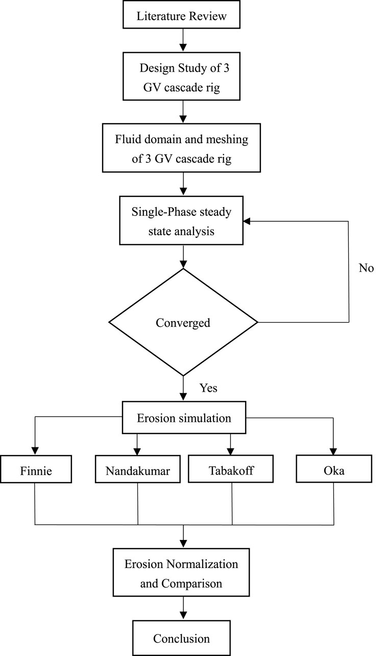
Figure 4. Methodology flow chart.

3.1 Numerical setup

The study involved developing a 3D model geometry of 3GV cascade rig, proper meshing the geometry, defining the proper boundary conditions, running the numerical simulation in OpenFOAM and interpreting the results. The numerical simulations were conducted using the open-source Computational Fluid Dynamics (CFD) software, OpenFOAM. OpenFOAM was chosen for its flexibility in modelling complex flows and its ability to handle multiphase flows with sediment transport. It also allowed for compilation of different erosion models.

3.1.1 Geometrical modelling and mesh

The design of 3GV cascade rig was obtained from the previous study (Chitrakar, 2018; Thapa et al., 2016). The 3GV cascade rig was designed to represent the GVs configuration in cascade and covered a section of the GV ring with three GVs. The sector covered was at the angle of 60°. It was designed to study the flow around the GV while minimizing the wall effects that were present in one GV rig (Chitrakar et al., 2017). The fluid domain consisted of three GVs of which the middle one has a 2 mm clearance gap on its one end.

The 3GV cascade rig geometry was discretized and accurately represented in the numerical model. The meshing tool available in OpenFOAM: snappyHexMesh, was used. It was refined near the walls and patches. Further refinement was done around the middle guide vane as well as the top wall, where the leakage flow is expected. Figure 5 and Table 1 shows the mesh statistics of the fluid domain.

Figure 5

Figure 5. (A) Fluid domain (B) Mesh around the guide vane of the 3 GV cascade rig.

Table 1

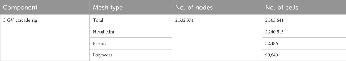
Table 1. Mesh statistics.

3.1.2 Boundary conditions

3.1.2.1 Inlet conditions

Inlet boundary conditions were specified to match that of previous research and actual site conditions. The flow rate of Jhimruk Hydropower is 2.35 m³/s for 24 guide vanes (Thapa et al., 2016). The fluid domain was designed for 4 passages so the flow rate was calculated to be 0.39167 m³/s. The “flowRateInletVelocity” with the volumetric flow rate of 0.39167 m³/s was specified as velocity inlet.

3.1.2.2 Outlet conditions

The pressure outlet of 1 atmospheric pressure was used as exit conditions as the fluid is released to the atmosphere.

3.1.2.3 Wall conditions

The GVs were treated as solid walls with no-slip boundary conditions. These are also the area of interest for erosion. Wall conditions were specified in the hub side plate, shroud side plate and the plates that govern the flow inside the cascade.

3.1.2.4 Sediment injection

Source terms were added at the sediment injection points to model sediment introduction into the flow. The sediments were introduced at the inlet. Since this is a qualitative study, the amount of erodent does not play a significant role in the result, hence they were iteratively changed such that a better qualitative understanding of the affected region could be obtained. However, a constant concentration was maintained across the cases where different erosion models were used. The particles with a size of 0.0025 mm were used, and were injected for 200 iterations after the flow had been stabilized. OpenFOAM quantifies erosion and stores it as “kinematicCloudQ”. The physical interpretation of “kinematicCloudQ” depends on the particular erosion model used to calculate it.

3.1.3 Numerical method

For the flow simulation, simpleFoam; a built in OpenFOAM solver was used. SimpleFoam is a steady-state solver for incompressible and turbulent flow. It uses SIMPLE or SIMPLEC algorithm. The solution strategy of simpleFoam involves sequential solving which means the solution from one equation is used for another. SimpleFoam solves the incompressible Navier-Stokes equations which explain how momentum is conserved in fluid flow and satisfies the continuity equation. This solver solves the equation in four steps. Firstly, the momentum equation is solved to get a diverged velocity value u*, here the diverged means it does not necessarily satisfy the continuity equation. After that, using the momentum and continuity equation, the pressure value p_n is obtained. The obtained pressure value is used to correct the velocity field and obtain divergence free velocity value u. These obtained values are then used to solve the turbulence equation. In order to observe erosion, a coupled solver was created. In this solver, simpleFoam solver was coupled with Lagrangian particles. By using such a coupled approach, the need for transient simulation to study erosion can be avoided, which reduces the computational time significantly. Convergence criteria for residual values were established to determine solution convergence. The solution of the study was deemed to converge when the residuals became less than 1e-5. The flow was solved for the velocity and other flow characteristics of the continuous media. The coupling then transferred the motion to the particle and hence calculated the forces acting on the particle. Then, the particle velocity and impingement angle on the walls were determined, which are the inputs required for the erosion model.

3.1.4 Erosion models

Along with Finnie erosion model, three other erosion models (Nandakumar, Tabakoff and Grant, and Oka) erosion models were used to compare and determine the suitable erosion model to predict erosion at the CG. The sediment particles’ behavior with the wall was governed by the “localWallInteraction” model. In OpenFOAM, the “particleErosion” template—which included the “ParticleErosion.H″ and “ParticleErosion.C″ files—was used to compile several erosion models and calculate erosion on specified territories. While “ParticleErosion.C″ included the actual source code for modelling material erosion caused by particle collisions, “ParticleErosion.H″ created prototypes of interfaces, data structures, and functions. This configuration made it possible to simulate and compare erosion patterns across many models with accuracy (Shrestha S. et al., 2024).

3.1.5 Material properties

Material properties of both the GVs and sediment particles, including erosion-related properties, were defined in the numerical model. The wall properties were specified in the terms of yield stress while the interaction was governed by the proportion between the cut’s depth and the depth of contact. The diameter, density, Young’s modulus and Poisson’s ratio were quantified for the particle. Here, the concentration of the particles, properties related to the sediments and end of injection of particles were also defined. The walls of interest, i.e., where the erosion is sought, was also specified here. For this study, the GV walls of the middle GV was defined as the wall of interest.

3.1.6 Normalization

Finnie erosion model (Finnie, 1960) calculates the volume of material eroded from the surface. Similarly, Tabakoff and Grant model (Grant and Tabakoff, 1973) calculates the erosion damage per unit mass of erodent. Nandakumar model (López et al., 1995) calculates volume eroded while Oka model (Oka et al., 1993) calculates the depth of erosion. Conversely, for the real case of eroded guide vane, depth was used to measure the amount of erosion. So, in order to compare the sediment erosion results of different erosion models, normalizing the value is important. Normalizing means dividing each value of “kinematicCloudQ” by the maximum value which gives the value between 0 and 1. The erosion is more severe if the normalized value is near 1, and less severe if the normalized value is near 0. So, in this way, less severe and more severe erosion was predicted. Normalization allowed the results obtained from different erosion models to be compared as all the values lay on the same scale of reference i.e., between 0 and 1.

3.1.7 Validation

The results found in literature were used to validate the findings of this study. The flow inside the 3GV cascade was validated using the results of numerical simulation and PIV (Chitrakar, 2018). After similar results were obtained in terms of flow velocity and flow pattern, an erosion study was conducted. The erosion observed in this study was compared with the real GV erosion for validation. The real GV erosion was analyzed for different depths of erosion.

4 Results and discussion

4.1 Flow analysis at the 3GV cascade rig

In order to validate the case, firstly the flow inside the cascade was needed to be verified. In order to achieve this, the flow obtained through previous research using ANSYS software and PIV was used as the basis for comparison. A previous study (Chitrakar et al., 2017) discussed the comparison between CFD and PIV in a single GV rig. The flow analysis was done in OpenFOAM, and was compared with past results where it was observed that the flow patterns were similar throughout the domain. Figure 6 shows the velocity contours at the midspan of the cascade rig. The previously obtained results (Chitrakar et al., 2019a; Chitrakar et al., 2019b) in Figure 6A are comparable to the OpenFOAM simulation results in Figure 6B also in critical areas like the leading edge where stagnation occurs, the profiles along the trailing edge, and the flows along the pressure and suction sides.

Figure 6

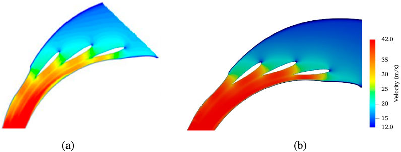
Figure 6. Velocity contour at midspan (A) ANSYS CFX simulation (Chitrakar et al., 2019a) (B) OpenFOAM simulation.

The velocity distribution was observed to be similar at the mid span of the guide vane. The stagnation point was obtained at the leading edge of the GV and a low velocity core was obtained at the trailing edge as well. The close resemblance of the flow field showed that the simulation matches the previous research (Chitrakar et al., 2017; Chitrakar et al., 2019a; Chitrakar et al., 2019b).

Figure 7 shows the comparison of velocity contour at the clearance gap in ANSYS CFX and PIV (Chitrakar et al., 2017) with OpenFOAM. In Figure 7, the velocity distribution within the clearance gap was observed, comparing data from both CFD and PIV. This velocity pattern was closely tied to the loading of the GV. Towards the Leading Edge (LE) of the GV, the flow inside the CG followed the primary mainstream flow. This occurs because the pressure difference in the LE region is relatively small compared to the region around the Trailing Edge (TE). In both CFD and PIV, accelerated flow near the TE was observed. However, in the case of PIV, the flow pattern appeared more irregular, likely due to the influence of nearby walls. These irregularities may also stem from induced cavitation within the low-pressure clearance area. The leakage flow depicted in Figure 7 combines with the Suction Side (SS) flow, creating a vortex filament that tends to shift towards the midspan as it travels downstream. It can thus be concluded that the flow in the CG was replicated in the study.

Figure 7

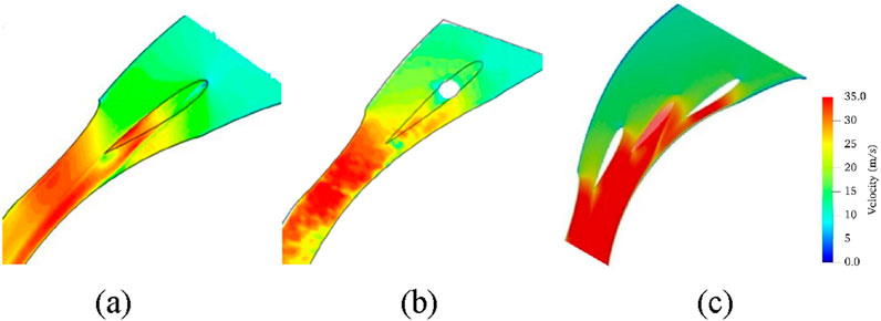
Figure 7. Velocity contour at clearance gap (A) ANSYS simulation (B) PIV (Chitrakar et al., 2017) (C) OpenFOAM simulation.

4.2 Erosion analysis for different erosion models

After verifying the flow field the sediment particles were introduced. These particles cause erosion in the area of interest. The value of erosion depends on the model of erosion used. As explained earlier, normalized value of the erosion was used for comparison between the erosion models. The erosion patterns observed for different erosion models are shown in Table 2. The suction side (concave) of the GV were observed to have more erosion than the pressure side (convex) of the GV.

Table 2

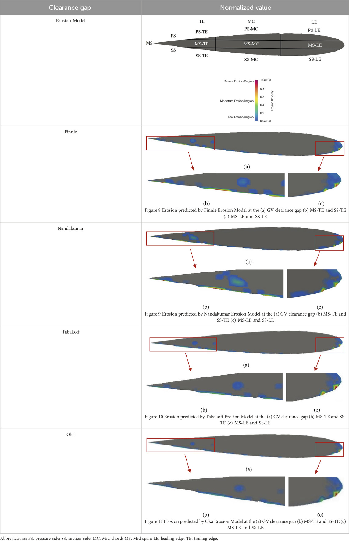
Table 2. Erosion at the clearance gap of GV.

Finnie erosion model (Finnie, 1960) is highly dependent on the impact angle, so it predicts maximum erosion at low impact angle. Finnie erosion model predicted severe erosion at the suction side (SS) of the LE of the CG. SS of the CG was also seen to have more erosion compared to the pressure side (PS). The trailing edge region of the suction side was also predicted to have severe erosion. Low erosion was observed at the other regions of the guide vane.

Nandakumar erosion model (López et al., 1995) is the modified version of the Finnie erosion model that considers the combined effects of multiple impacts and energy-dissipation process. Nandakumar erosion model also predicted the LE of the SS of the CG to have severe erosion along with the TE. In addition to that, medium erosion was predicted between the PS and SS of the TE as shown in Table 2. This erosion maybe due to the leakage flow vortex at the CG of the GV as shown in flow analysis in Figure 7.

Tabakoff and Grant erosion model (Grant and Tabakoff, 1973) is also sensitive to the impact angle and the particle velocity. This erosion model also predicted the erosion at the LE of the SS inside the CG to be the most severe as shown in Table 2. Other regions of the CG were predicted to have medium to low erosion.

For Oka erosion model (Oka et al., 1993) the most sensitive property is the particle velocity. Oka erosion model also predicted the erosion at the LE of the SS of the CG to be the most severe as shown in Table 2. Other regions were predicted as the low and medium erosion regions by Oka erosion model.

4.3 Erosion wear comparison with actual eroded guide vane

The reference for this study is Jhimruk HEP which has 24 GVs. All the GVs suffered erosion which were similar in nature to each other after operating in sediment laden flow for a certain period. While some particular details might be different, the overall erosion was comparable in the set of GVs used at Jhimruk HEP. Other hydropower plants with differing configuration was also observed to have similar erosion pattern in their GVs. In previous study, one of the eroded GV with 3D scan of Jhimruk HEP was used (Aryal et al., 2020). In this study, the same 3D scanned GV geometry was used for analysis. The GV had enlarged CG in each side and both these sides were used for comparison with the numerically predicted results (Aryal et al., 2020). The severity of erosion was obtained by comparing the eroded 3D scanned geometry with the non eroded GV. Similar to the CFD results, the erosion observed in the actual GV of Jhimruk HEP were normalized and classified. The actual GVs have shafts to allow for movement. In order to meet the structural integrity, the diameter of the shaft is larger than the thickness of the GV, so flange like structures are provided to accommodate the shaft. The comparison of the eroded GV with the non-eroded GV showed that at the lower side of the CG, the erosion was observed to be the most severe in LE of the SS, the flange on the SS, part of the flange in the PS and at the very edge of the TE of the SS. Moderate erosion was observed between PS and SS, ahead of the shaft. The erosion was observed to be uniform on the upper and lower CGs. The only difference was observed in the mid span region near the LE where the upper CG had low erosion, but the lower CG had severe erosion. Tables 2, 3 shows the erosion damages at the clearance gap of the GV of Jhimruk HEP.

Table 3

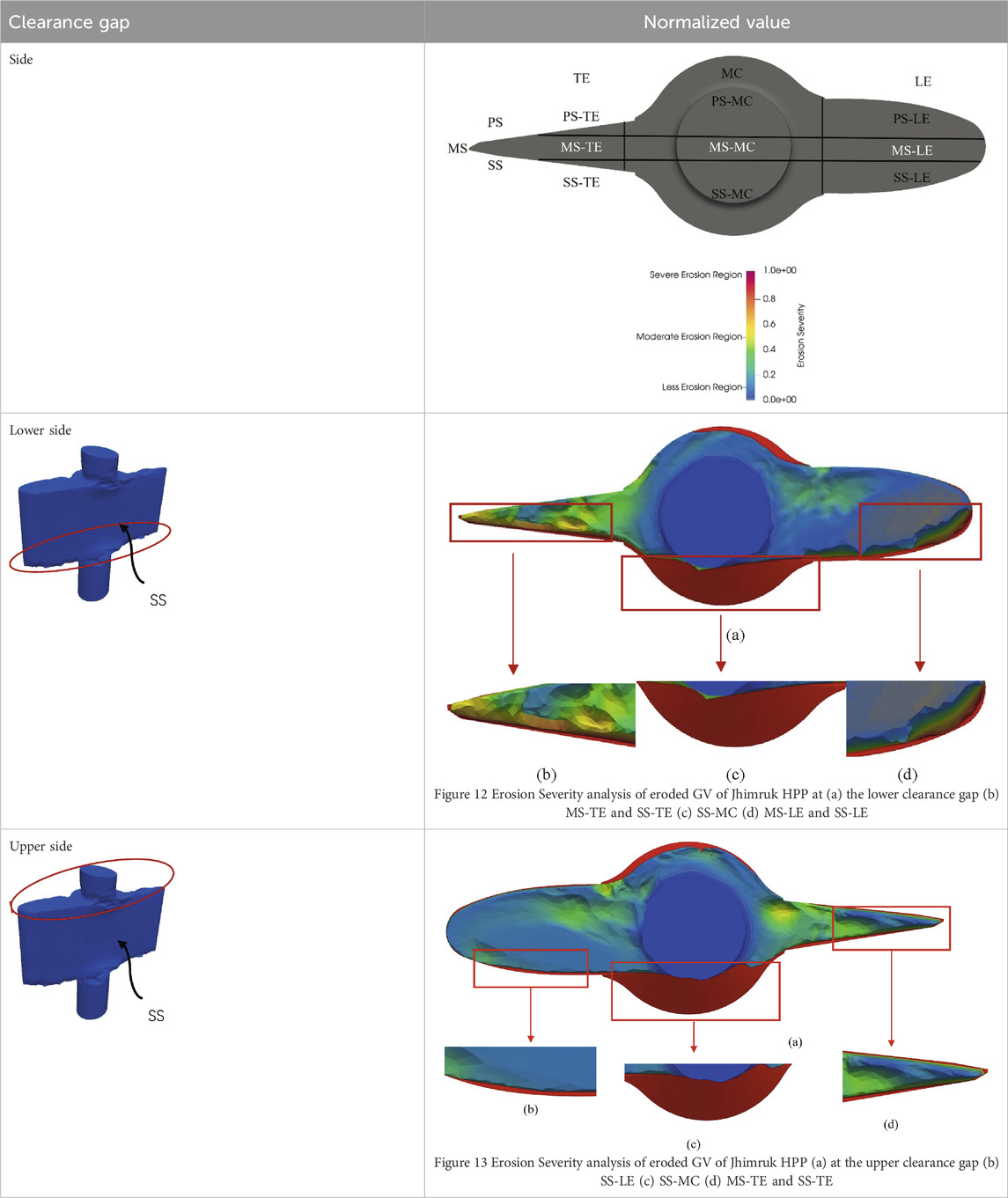
Table 3. Analysis of the real case erosion of guide vane.

On comparing the levels of erosion observed from the numerical results and the actual scanned model it was observed that different models could predict the severity of different locations. The severe erosion observed at the SS-TE (suction side of leading edge) of the clearance gap was predicted as severe level of erosion by Finnie, Tabakoff and Grant, and Oka erosion models. Nandakumar erosion model was able to predict only a small area as severe erosion and predicted the other regions to be as moderate erosion region. Finnie erosion model was able to predict the predominant erosion region accurately. Similarly, the severe erosion of the SS-TE was predicted accurately by both Finnie and Nandakumar erosion models comparing to eroded GV. Tabakoff and Grant, and Oka erosion models predicted the region as the low erosion region.

The moderate erosion downstream of the mid chord region was observed in real case. This was predicted as less erosion region by most erosion models. However, Nandakumar erosion model predicted it as the most predominant region of erosion and also predicted greater severity of erosion in this region.

The erosion at the SS of the TE (SS-TE) of the GV was observed to be severe in the both upper side and lower side in eroded GV. Tabakoff and Grant erosion model and Oka erosion model predicted the least severity of erosion in this region. However, the erosion was predicted as severe by Finnie erosion model and Nandakumar erosion model. Hence, both Finnie model and Nandakumar model were able to predict the erosion in this region.

In case of the overall LE, the area of erosion predicted by Finnie was less severe erosion, which was observed to be higher than the other three erosion models. This was similar to the mild erosion observed in the LE region of the actual eroded GV as seen at the upper side. By comparing results with the actual eroded GV, Finnie erosion model was observed to predict the severe erosion at the leading edge of the suction side (SS-LE), less severe erosion in the LE region and severe erosion at the trailing edge of the suction side (SS-TE). In the mid-chord region, Nandakumar erosion model was able to predict medium erosion which was similar to the eroded GV. Table 4 shows the evaluation of different erosion models with the actual eroded GV.

Table 4

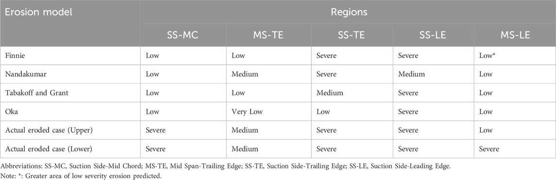
Table 4. Evaluation of the erosion models.

4.4 Implications and future recommendations

The CG of the GV is one of the most vulnerable regions of erosion in Francis turbine. Therefore, an accurate prediction of the erosion in this region is required to accurately plan for the prevention approaches. The numerical investigations using the 3GV cascade rig yielded good adherence to flow results, hence it was chosen as an effective method to predict the erosion pattern in GV of Francis turbine.

This study could be significant for guide vane optimization and coating areas where the erosion is substantial to elongate the life of the GV of Francis turbine. Experimental studies could be done in 3GV cascade rig to test the GVs in different operating conditions to identify the significance of flow rates, GV angles and other parameters on GV erosion. Other factors, such as cavitation could also be the cause of surface deformation. Many studies have considered erosion, cavitation and their coalesced effect (Vite-Torres et al., 2022; Gohil and Saini, 2014; Roa et al., 2015). The 3D scanned geometry and its deformed contours that have been formed due to erosion was considered in this study. Additionally, the deformation could possibly have been due to cavitation or combined effect of cavitation and erosion, both of which have not been considered in this study.

Numerically, only initial erosion was studied. But eroded surface leads to deformation, which will alter the flow and introduce other forms and locations of erosion. Deformation study could be considered for future study similar to Shrestha K. et al. (2024). Experimental studies over various operating parameters could further enhance the results of this study. By using erosive particles, the erosion prone areas can be identified in a controlled manner.

5 Summary and conclusion

This study compared numerical simulation using different erosion models implemented at the clearance gap of the GV using the simplified 3GV cascade rig fluid domain designed from the turbine setup of Jhimruk HEP and the sediment concentration similar to that found in the same HEP. A fluid domain based on the previous experimental setup of 3GV cascade rig was created in which, the meshing was done using the OpenFOAM snappyHexMesh.

Four different erosion models namely, Finnie, Nandakumar, Tabakoff and Grant, and Oka erosion models were considered for erosion simulation. The following conclusions were drawn from this study:

• Overall, the most severely eroded region of the clearance gap of the GV was found to be the suction side of the trailing edge (SS-TE) and the suction side of the leading edge (SS-LE).

• The analysis of the actual eroded case of the Jhimruk HEP also showed that the SS-LE and SS-TE are the most severely affected regions of the clearance gap of GV.

• The other region where significant erosion was seen is the region around the trailing edge, pressure side and the mid-span around the shaft region.

• Among the erosion models, Nandakumar erosion model was able to predict the erosion around the trailing edge.

• Finnie erosion model was able to predict severe erosion at the leading-edge suction side (SS-LE) and severe erosion at the trailing edge of the suction side (SS-TE) more precisely, when compared to actual eroded GV.

• By overall comparison with the actual eroded GV it can be said that Finnie erosion model was best suited among the implemented erosion models to observe the erosion pattern for the clearance gap of the GV. This result emphasizes the suitability of Finnie erosion model for erosion prediction at low impact angle.

Data availability statement

The raw data supporting the conclusions of this article will be made available by the authors, without undue reservation.

Author contributions

RS: Data curation, Formal Analysis, Investigation, Methodology, Software, Validation, Visualization, Writing–original draft, Writing–review and editing. KS: Data curation, Formal Analysis, Investigation, Methodology, Software, Validation, Visualization, Writing–original draft, Writing–review and editing. SC: Conceptualization, Funding acquisition, Project administration, Supervision, Validation, Writing–review and editing. BT: Conceptualization, Funding acquisition, Project administration, Supervision, Validation, Writing–review and editing. HN: Conceptualization, Funding acquisition, Project administration, Supervision, Validation, Writing–review and editing. ZQ: Conceptualization, Funding acquisition, Project administration, Supervision, Validation, Writing–review and editing. ZG: Conceptualization, Funding acquisition, Project administration, Supervision, Validation, Writing–review and editing.

Funding

The author(s) declare that financial support was received for the research, authorship, and/or publication of this article. This study was performed jointly at Turbine Testing Lab, Kathmandu University and State Key Laboratory of Water Resources Engineering and Management, Wuhan University. The project was supported by Visiting Scholar’s Fund provided by WRHES, China (Project No. 2021SDG01), TTL-Fault (ENEP-RENP-II-23-03), and Hydro Himalaya (NORHED-II) Project.

Conflict of interest

The authors declare that the research was conducted in the absence of any commercial or financial relationships that could be construed as a potential conflict of interest.

Generative AI statement

The author(s) declare that no Generative AI was used in the creation of this manuscript.

Publisher’s note

All claims expressed in this article are solely those of the authors and do not necessarily represent those of their affiliated organizations, or those of the publisher, the editors and the reviewers. Any product that may be evaluated in this article, or claim that may be made by its manufacturer, is not guaranteed or endorsed by the publisher.

Abbreviations

GV, Guide Vane; CG, Clearance Gap; CFD, Computational Fluid Dynamics; PIV, Particle Image Velocimetry; RANS, Reynold Averaged Navier Stokes; SST, Shear Stress Transport; PS, pressure side; SS, suction side; MC, Mid-chord; MS, Mid-span; LE, leading edge; TE, trailing edge; OpenFOAM, Open Field Operation And Manipulation; HEP, Hydro-electric Plant.

References

Acharya, N., Trivedi, C., Wahl, N. M., Gautam, S., Chitrakar, S., and Dahlhaug, O. G. (2019). Numerical study of sediment erosion in guide vanes of a high head Francis turbine. J. Phys. Conf. Ser. 1266, 012004. doi:10.1088/1742-6596/1266/1/012004

CrossRef Full Text | Google Scholar

Anderson, J. D. (1995). Computational fluid dynamics-the basic applications. Singapore: McGraw-Hill, Inc.

Google Scholar

Aryal, S., Chitrakar, S., Shrestha, R., and Jha, A. K. (2020). A case study of wear in a high head francis turbine due to suspended sediment and secondary flow in a hydropower plant of Nepal. Int. J. Fluid Mach. Syst. 13 (4), 692–703. doi:10.5293/IJFMS.2020.13.4.692

CrossRef Full Text | Google Scholar

Bansal, R. K. (2010). A textbook of fluid mechanics and hydraulic machines. Delhi: Laxmi Publications Pvt. Ltd.

Google Scholar

Bardal, E. (1985). Korrosjon og korrosjonsvern.

Google Scholar

Burwell, J.Jr. (1957). Survey of possible wear mechanisms. Wear 1, 119–141. doi:10.1016/0043-1648(57)90005-4

CrossRef Full Text | Google Scholar

Chitrakar, S. (2018). Secondary flow and sediment erosion in Francis turbines. Trondhein: Norwegian University of Science and Technology. Doctoral Thesis.

Google Scholar

Chitrakar, S., Dahlhaug, O. G., and Neopane, H. P. (2018b). Numerical investigation of the effect of leakage flow through erosion-induced clearance gaps of guide vanes on the performance of francis turbines. Eng. Appl. Comput. Fluid Mech. 12 (1), 662–678. doi:10.1080/19942060.2018.1509806

CrossRef Full Text | Google Scholar

Chitrakar, S., Neopane, H. P., and Dahlhaug, O. G. (2016). Study of the simultaneous effects of secondary flow and sediment erosion in Francis turbines. Renewable Energy 97 1–11. doi:10.1016/j.renene.2016.06.007

CrossRef Full Text | Google Scholar

Chitrakar, S., Neopane, H. P., and Dahlhaug, O. G. (2018a). “A review on sediment erosion challenges in hydraulic turbines,” in Sedimentation engineering (InTech). 10.5772/intechopen.70468

Google Scholar

Chitrakar, S., Neopane, H. P., and Dahlhaug, O. G. (2019a). The numerical and experimental investigation of erosion induced leakage flow through guide vanes of Francis turbine. IOP Conf. Ser. Earth Environ. Sci. 240, 072002. doi:10.1088/1755-1315/240/7/072002

CrossRef Full Text | Google Scholar

Chitrakar, S., Neopane, H. P., and Dahlhaug, O. G. (2019b). Development of a test rig for investigating the flow field around guide vanes of Francis turbines. Flow Meas. Instrum. 70, 101648. doi:10.1016/j.flowmeasinst.2019.101648

CrossRef Full Text | Google Scholar

Chitrakar, S., Thapa, B. S., Dahlhaug, O. G., and Neopane, H. P. (2017). Numerical and experimental study of the leakage flow in guide vanes with different hydrofoils. J. Comput. Des. Eng. 4 (3), 218–230. doi:10.1016/j.jcde.2017.02.004

CrossRef Full Text | Google Scholar

Finnie, I. (1960). Erosion of surfaces by solid particles. Wear 3, 87–103. doi:10.1016/0043-1648(60)90055-7

CrossRef Full Text | Google Scholar

Gohil, P. P., and Saini, R. P. (2014). Coalesced effect of cavitation and silt erosion in hydro turbines - a review. Renewable and Sustainable Energy Reviews 33, 280–289. doi:10.1016/j.rser.2014.01.075

CrossRef Full Text | Google Scholar

Grant, G., and Tabakoff, W. (1973). An experimental investigation of the erosive characteristics of 2024 aluminum alloy. Cincinnati, Ohio: Cincinnati University.

Google Scholar

IEC (2009). Hydraulic machines e guide for dealing with abrasive erosion in water. 62364 Ed. 1.0.

Google Scholar

Kang, M. W., Park, N., and Suh, S. H. (2016). Numerical study on sediment erosion of francis turbine with different operating conditions and sediment inflow rates. Procedia Eng. 157, 457–464. doi:10.1016/j.proeng.2016.08.389

CrossRef Full Text | Google Scholar

Kapali, A., Chitrakar, S., Shrestha, O., Neopane, H. P., and Thapa, B. S. (2019). A review on experimental study of sediment erosion in hydraulic turbines at laboratory conditions. J. Phys. Conf. Ser. 1266, 012016. doi:10.1088/1742-6596/1266/1/012016

CrossRef Full Text | Google Scholar

Koirala, R., Neopane, H. P., Zhu, B., and Thapa, B. (2019). Effect of sediment erosion on flow around guide vanes of Francis turbine. Renew. Energy 136, 1022–1027. doi:10.1016/j.renene.2019.01.045

CrossRef Full Text | Google Scholar

Koirala, R., Thapa, B., Neopane, H. P., and Zhu, B. (2017). A review on flow and sediment erosion in guide vanes of Francis turbines. Renewable and Sustainable Energy Reviews 75, 1054–1065. doi:10.1016/j.rser.2016.11.085

PubMed Abstract | CrossRef Full Text | Google Scholar

Kumar Sahu, R., and Kumar Gandhi, B. (2022). Erosive flow field investigation on guide vanes of Francis turbine – a systematic review. Sustain. Energy Technol. Assessments 53, 102491. doi:10.1016/J.SETA.2022.102491

CrossRef Full Text | Google Scholar

Lenarcic, M., Eichhorn, M., Schoder, S. J., and Bauer, C. (2015). Numerical investigation of a high head Francis turbine under steady operating conditions using foam-extend. J. Phys. Conf. Ser. 579, 012008. doi:10.1088/1742-6596/579/1/012008

CrossRef Full Text | Google Scholar

López, A., Stickland, M. T., and Dempster, W. M. (1995). Comparative study of different erosion models in an Eulerian-Lagrangian frame using Open Source software.

Google Scholar

Noon, A. A., and Kim, M. H. (2021). Sediment and cavitation erosion in Francis turbines—review of latest experimental and numerical techniques. MDPI AG. doi:10.3390/en14061516

CrossRef Full Text | Google Scholar

Oka, Y. I., Matsumura, M., and Kawabata, T. (1993). Relationship between surface hardness and erosion damage caused by solid particle impact. Wear 162-164, 688–695. doi:10.1016/0043-1648(93)90067-V

CrossRef Full Text | Google Scholar

Rakibuzzaman, M., Kim, H. H., Kim, K., Suh, S. H., and Kim, K. Y. (2019). Numerical study of sediment erosion analysis in Francis turbine. Sustain. Switz. 11 (5), 1423. doi:10.3390/su11051423

CrossRef Full Text | Google Scholar

Roa, C. V., Muñoz, J., Teran, L., Valdes, J., Rodríguez, S., Coronado, J., et al. (2015). Effect of tribometer configuration on the analysis of hydromachinery wear failure. Wear 332–333, 1164–1175. doi:10.1016/J.WEAR.2015.01.068

PubMed Abstract | CrossRef Full Text | Google Scholar

Shrestha, K., Bijukchee, P. L., Thapa, B., Chitrakar, S., Guo, Z., and Qian, Z. (2024b). Numerical study of flow phenomena and erosion in three guide vane cascade rig. IOP Conf. Ser. Earth Environ. Sci. 1411 (1), 012010. doi:10.1088/1755-1315/1411/1/012010

CrossRef Full Text | Google Scholar

Shrestha, S., Bijukchhe, P. L., Chitrakar, S., Thapa, B., Qian, Z., and Guo, Z. (2024a). Comparative study of different erosion models in francis runner blade using OpenFOAM. IOP Conf. Ser. Mater Sci. Eng. 1314 (1), 012009. doi:10.1088/1757-899X/1314/1/012009

CrossRef Full Text | Google Scholar

Shrestha, U., Chen, Z., Park, S. H., and Do Choi, Y. (2019). Numerical studies on sediment erosion due to sediment characteristics in Francis hydro turbine. IOP Conf. Ser. Earth Environ. Sci. 240, 042001. doi:10.1088/1755-1315/240/4/042001

CrossRef Full Text | Google Scholar

Stojanovic, B., and Ivanovic, L. (2014). Tribomechanical systems in design. Journal of the Balkan Tribological Association 20 (1), 25–34.

Google Scholar

Thapa, B. (2004a). Sand erosion in hydraulic machinery. PhD Thesis. Trondheim, (Norway): NTNU.

Google Scholar

Thapa, B. S., Thapa, B., and Dahlhaug, O. G. (2012). Empirical modelling of sediment erosion in Francis turbines. Energy 41 (1), 386–391. doi:10.1016/j.energy.2012.02.066

CrossRef Full Text | Google Scholar

Thapa, B. S., Trivedi, C., and Dahlhaug, O. G. (2016). Design and development of guide vane cascade for a low speed number Francis turbine. J. Hydrodynamics 28 (4), 676–689. doi:10.1016/S1001-6058(16)60648-0

CrossRef Full Text | Google Scholar

Tsuguo, N. (1999). “Estimation of repair cycle of turbine due to abrasion caused by suspended sand and determination of desilting basin capacity,” in Proceedings of international seminar on sediment handling technique (Kathmandu: NHA).

Google Scholar

Vite-Torres, M., Moreno-Ríos, M., Villanueva-Zavala, A., Gallardo-Hernández, E. A., Farfán-Cabrera, L., and Mesa-Grajales, D. H. (2022). Study of cavitation erosion phenomenon at stainless steel AISI 304 base and with SiC coating. Appl. Eng. Lett. 7 (2), 67–73. doi:10.18485/aeletters.2022.7.2.3

CrossRef Full Text | Google Scholar

Winkler, K. (2014). Hydro-abrasive erosion: problems and solutions. IOP Conf. Ser. Earth Environ. Sci. 22, 052022. doi:10.1088/1755-1315/22/5/052022

CrossRef Full Text | Google Scholar