Precision assembly error analysis of parts based on multi-constraint surface matching

Existing assembly analysis methods often fail to accurately capture the complexities involved in the precision assembly of real-world parts. This paper introduces an advanced precision assembly error analysis method based on multi-constraint surface matching, aimed at overcoming these limitations. The proposed approach incorporates interference-free constraints and force stability constraints to develop an assembly positioning model that better reflects the realistic assembly process. To solve the model, Spatial Pyramid Matching with chaotic mapping is employed for population initialization, thereby enhancing population diversity. A nonlinear control mechanism is further introduced to dynamically adjust inertia weight, and a simulated annealing mechanism is integrated into the particle swarm optimization algorithm to enhance the efficiency of the surface matching process. The method ultimately achieves high-precision multi-constraint surface matching and completes a comprehensive assembly error analysis. The effectiveness and enhanced performance of the proposed methodology are validated through the precision assembly of a vibratory bowl feeder, demonstrating its potential to significantly improve assembly accuracy in precision manufacturing contexts.

1 Introduction

In aerospace, precision instruments, and high-end equipment manufacturing, precision assembly of parts is a critical factor in ensuring product quality and performance (Yi et al., 2024). Precision assembly involves assembling multiple finely machined parts according to specific technological procedures to form a complete unit. Its success depends on establishing precise fitting relationships between the surfaces of different components (Liu et al., 2023). However, due to machining errors, part surfaces often exhibit uneven geometric features at the micro-scale, leading to deviations from the ideal condition when two mating surfaces are joined, which results in assembly errors. Furthermore, these assembly errors can propagate and accumulate through multiple mating constraints within the assembly, posing significant challenges to overall assembly quality (Zhang et al., 2019). If the assembly quality is unqualified, it will result in higher costs and time losses (Vashishtha et al., 2025a; Chauhan et al., 2024). Thus, investigating the matching issues between imperfect part surfaces is a crucial aspect of assembly analysis, offering valuable insights into the impact of machining errors on assembly quality.

Converting the assembly error analysis problem into a surface matching problem has gained significant attention from researchers both domestically and internationally, becoming a promising research direction. Currently, surface matching studies in the field of assembly error analysis can be broadly categorized into two types: unconstrained surface matching and constrained matching. Han et al. (2016), Wu et al. (2020), and Jingyu et al. (2023) have used unconstrained surface matching methods to solve the assembly error analysis problem. Their core idea is to transform the surfaces of two mating parts into point sets and then use the Iterative Closest Point (ICP) to determine the correspondence and transformation matrix between the point sets (Pottmann et al., 2006). While the proposed surface matching model is simple and highly general, it oversimplifies the surface matching process during assembly, leaving room for improvement in computational accuracy (HAN et al., 2016). Cheng et al. (2024), Zhang et al. (2024), and Tian et al. (2023) have addressed the shortcomings of the ICP algorithm by replacing the point-to-point nearest distance with a point-to-surface nearest distance method, thereby improving calculation accuracy. These unconstrained surface matching algorithms only consider the Euclidean distance between two surfaces, which involves overly idealized assumptions and neglects engineering constraints present during the assembly process. To address these limitations, Yan and Ballu, (2018) and Schleich and Wartzack, (2018) used skin models to represent surfaces of parts with errors, integrating interference-free constraints into the surface matching process. Zhang et al. (2018) replaced the original surfaces of parts with two substitute surfaces and introduced a surface constraint-based matching algorithm. To demonstrate its effectiveness, an example involving the assembly of two cylindrical workpieces was used to show that this method can better reflect the actual contact state. Results indicate that considering interference-free constraints more accurately reflects real-world scenarios. Sun et al. (2019) and Zhang, (2016) further incorporated force stability constraints in three-point contact alongside interference-free constraints, calculating the optimal contact state of the part surfaces. They used the relative error between the substitute surface formed by contact points and the ideal surface to represent assembly error. Furthermore, Sun Q and his team employed the processing characteristics of a certain gyroscope and conducted strategic experimental validation. The experimental results demonstrated that this method is effective in improving assembly accuracy. This approach extends the engineering constraints required for surface matching but is limited to matching between a curved surface and a plane, as well as three-point contact between the two surfaces. In conclusion, comprehensively considering engineering constraints during the surface matching process is crucial to enhancing the accuracy of assembly error analysis. However, current research is still insufficient, mainly reflected in the following aspects: many researchers focus only on minimizing the closest distance between surfaces, leading to results inconsistent with the actual physical assembly process. While some researchers have considered either interference-free constraints or force stability constraints—or both—their methods are not yet applicable to broader and more complex surface-to-surface matching situations. Therefore, exploring advanced technologies and methodologies is crucial for effectively addressing this issue (Vashishtha et al., 2025b). In view of this, this paper takes into account non-interference constraints and force stability constraints, aiming to reflect a more realistic part assembly process and improve assembly accuracy. At the same time, this method is also applicable to the matching between curved surfaces.

Surface matching is a crucial research area in assembly error analysis, aiming to establish a quantitative relationship between machining errors and assembly errors. The least squares method and intelligent optimization algorithms are two prominent approaches for solving these models, both of which have made significant progress in the field. Wen et al. (2009) and Chen et al. (2023) utilized the least squares method to calculate the optimal transformation matrix between point sets, achieving assembly positioning for two surfaces and determining part assembly errors, with experimental results demonstrating good performance. Wei W (Wv et al., 2024) applied the least squares method to determine the actual fitting clearance of mating surfaces, constructed an error model for planar and cylindrical features based on error characterization methods, and verified its effectiveness using a servo system. Although the least squares method has shown good performance in model solving, it requires gradient information, which makes it challenging for complex models. Additionally, this method is not suitable for solving constrained problems. In contrast, intelligent optimization algorithms have broader applications in assembly error analysis. Zhang et al. (2007) employed particle swarm optimization (PSO) to evaluate errors and conducted comparative experiments with the least squares method, genetic algorithms, and other techniques, demonstrating superior accuracy. Yongsheng et al. (2023) combined genetic algorithms with simulated annealing to measure the matching between tooth surfaces and theoretical tooth surfaces, with experiments indicating that the algorithm could compensate for over 55% of measurement errors. However, the genetic algorithm used in that study involved complex encoding structures and multiple steps such as crossover and mutation. Guokai et al. (2022) utilized PSO to solve the assembly positioning model for 3D point cloud data, with experimental results showing significant improvement in accuracy. This method is straightforward, flexible in parameter adjustment, and achieves high accuracy in model solving, making it advantageous for assembly error analysis. Therefore, this paper adopts PSO as the solution algorithm for the surface matching model. Considering that this study focuses on matching between two complex surfaces and involves multiple engineering constraints, which may lead the algorithm to fall into local optima, we propose an improved algorithm based on the fundamental PSO algorithm from references (Wang et al., 2018; Lin et al., 2022) to enhance its applicability.

This paper presents a precision assembly error analysis method for parts based on multi-constraint surface matching. In Section 1, we introduce interference-free and force stability constraints to establish an assembly positioning model, incorporating multiple surface matching constraints. Corresponding penalty terms are used for these constraints, and the penalty function method is applied to transform the constrained problem into an unconstrained one. In Section 2, we propose an approach utilizing Spatial Pyramid Matching (SPM) with chaotic mapping for population initialization to enhance population diversity. To address the susceptibility of the basic particle swarm optimization (PSO) algorithm to local optima, we introduce a dynamic inertia weight adjustment method using a hyperbolic tangent function, and incorporate a simulated annealing mechanism into the PSO to avoid convergence to local optima. The improved PSO algorithm is then used to solve the model. In Section 3, we use a precision-machined vibratory bowl feeder as the case study and design three sets of experiments to evaluate the effectiveness of the proposed method and the performance of the improved PSO algorithm.

2 Assembly positioning based on multi-constraint surface matching

As illustrated in Figure 1, the assembly positioning process involves translating and rotating the surface to be matched from its initial position to the target surface, subject to various engineering constraints, to achieve optimal alignment between the mating surfaces. The key steps of this process are as follows: First, sampling is performed to generate 3D point cloud data, followed by meshing to convert the data into a triangular mesh model. Subsequently, under interference-free and force stability constraints, the nearest distances from the 3D point cloud to the triangular mesh are calculated to establish corresponding point sets, referred to as the source point set and the target point set. Finally, iterative translation and rotation are applied to continuously adjust the position of the source point set, ensuring optimal alignment with the target point set.

Figure 1

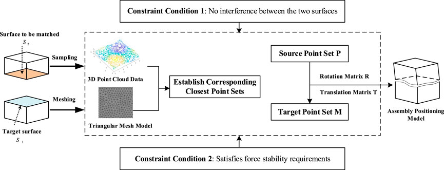
Figure 1. Assembly positioning process based on multi-constraint surface matching.

2.1 Establishment of assembly positioning model based on multi-constraint surface matching

The assembly positioning process based on multi-constraint surface matching is illustrated in Figure 2, with the detailed steps as follows:

(1) Surface Data Acquisition and Preprocessing. Identify the two mating surfaces with machining errors—target surface—target surface $S_1$ and the surface to be matched $S_2$. Convert target surface $S_1$ into a triangular mesh model $M=\left\{M_1\right.,M_2,...,M_i,...,M_{n-1},\left.M_n\right\}$, where $M_i$ represents the ith triangular mesh, and $n$ denotes the total number of triangular meshes. For surface $S_2$, obtain 3D point cloud data through sampling, with the point set denoted as $P=\left\{P_1\right.,P_2,...,P_i,...,P_{m-1,}\left.P_m\right\}$, where $P_i$ represents the jth point in the point cloud, and $m$ represents the total number of points in the point cloud.

(2) Calculate the nearest distances from the point cloud to the triangular mesh to establish the corresponding nearest point sets between the target surface $S_1$ and the surface to be matched $S_2$, namely, the target point set $M_{i,0}$ and the source point set $P_{i,0}$. $M_{i,0}$ and $P_{i,0}$ represent the initial correspondences between the target surface $S_1$ and the surface to be matched $S_2$ in their initial positions.

(3) Calculate the homogeneous transformation matrix for point set $P$ to ensure it meets the objective function (1) under interference-free and force stability constraints. These two constraints are explained in detail in Section 2.2.

$F\left(T_k,R_k\right)=\min {\displaystyle \frac{1}{m}\sum _{i=1}^m}{\displaystyle ||R_k{P}_{i,k-1}+T_k-M_{i,k}||}(1)$

Figure 2

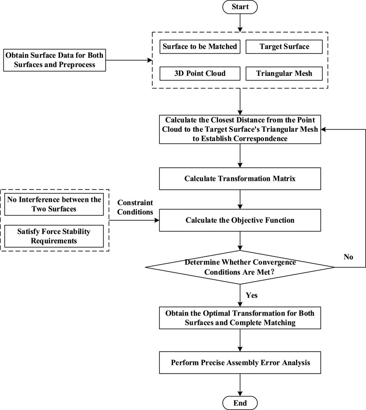
Figure 2. Assembly positioning based on multi-constraint surface registration.

In this formula, $R_k$ represents the optimal rotation matrix, whose expression is given by Equation 2. $\alpha$, $\beta$ and $\gamma$ denote the rotation angles of the point set around the x-axis, y-axis, and z-axis, respectively. $T_k$ represents the optimal translation matrix, whose expression is given by Equation 3. $t_x$, $t_{\mathrm{y}}$ and $t_z$ represent the translation distances of the point set along the x-axis, y-axis, and z-axis, respectively. $F\left(T_k,R_k\right)$ is the average distance from all transformed 3D point cloud data points p, after translation and rotation, to the nearest triangular mesh.

$R_k=\left[\begin{array}{ccc}\begin{array}{l}\cos \beta \cos \gamma \\ \cos \beta \sin \beta \\ -\sin \beta \end{array}& \begin{array}{l}\sin \alpha \sin \beta \cos \gamma -\cos \alpha \sin \beta \\ \sin \alpha \sin \beta \sin \gamma +\cos \alpha \cos \gamma \\ \sin \alpha \cos \beta \end{array}& \begin{array}{l}\cos \alpha \sin \beta \cos \gamma +\sin \alpha \sin \beta \\ \cos \alpha \sin \beta \sin \gamma -\sin \alpha \cos \beta \\ \cos \beta \cos \beta \end{array}\end{array}\right](2)$

$T_k=\left[\begin{array}{l}{t}_x\\ t_y\\ t_z\end{array}\right](3)$

(4) Transform the source point set $P_{i,k-1}$ through coordinate transformation to form a new point set, updating the position of all 3D point cloud data on surface $S_2$, denoted as $P_{i,k}=R_k{P}_{i,k-1}+T_k$. Then, based on the triangular mesh model, determine the nearest point from point cloud to each triangular mesh to calculate the objective function, whose expression is given by Equation 4:

$F_k=\min {\displaystyle \frac{1}{m}\sum _{i=1}^m}||P_{i,k}-M_{i,k}||(4)$

Where $‖P_{i,k}-M_{i,k}‖$ represents the Euclidean distance between points $P_{i,k}$ and $M_{i,k}$ at the kth iteration, and $‖·‖$ denotes the L2-norm.

(5) Termination Condition Evaluation. If $F_k$ is greater than or equal to the given threshold $\epsilon$, return to Step 3, and continue until the distance meets the requirement or the maximum number of iterations is reached.

(6) Calculate the final contact points between the target surface $S_1$ and the surface to be matched $S_2$, and perform assembly error analysis.

2.2 Constraint conditions

In practical assembly processes, the alignment of two surfaces involves more than simple positioning; it must also satisfy a set of defined engineering constraints. In this study, interference-free and force stability constraints are systematically introduced during each iteration to achieve a more accurate and realistic representation of the actual assembly conditions.

(1) Constraint Condition 1: During the matching process, the target surface $S_1$ and the surface to be matched $S_2$ must remain interference-free, i.e., no overlapping or intersection occurs between them. Mathematically, this condition is represented as $d_i\ge 0$, where $d_i$ denotes the minimum distance from a point on the source surface to the triangular mesh of the target surface.

The specific approach to determine whether this condition is satisfied is as follows: if a point lies on the side of the triangular mesh where the normal vector is directed, the distance from the point to the mesh is considered positive. As illustrated in Figure 3, positions 1, 2, and 3 exhibit $d_i<0$, indicating a violation of the constraint, whereas position four shows $d_i\ge 0$, thereby satisfying the constraint.

Figure 3

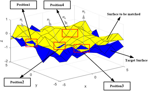
Figure 3. Non-interference schematic diagram.

To address Constraint Condition 1, this study utilizes the absolute value of the nearest distance from point cloud data points to the surface as a penalty term, formulating the penalty expression as shown in Equation 5.

$penalty1=\left\{\begin{array}{l}0,d_i\ge 0\\ \left|\min \left(dis\tan ces1\right)\right|,d_i<0\end{array}\right.(5)$

In this context, $\left|\min \left(dis\tan ces1\right)\right|$ represents the absolute value of the signed nearest distance from a point cloud data point to surface $S_1$. If $d_i\ge 0$, it indicates that there is no interference between the two surfaces, $penalty1=0$; whereas if $d_i<0$, it suggests that interference occurs between the two surfaces, $penalty1=\left|\min \left(dis\tan ces1\right)\right|$.

(2) Constraint Condition 2: During the assembly positioning process, force stability must be ensured. Force stability refers to the ability of components to maintain a stable state under certain conditions, which can be analyzed through the contact state of two surfaces. The contact states between two surfaces can be categorized as single-point contact (see Figure 4), two-point contact (see Figure 5), and multi-point contact (see Figures 6, 7). Single-point contact may lead to instability due to potential rotation of the surface around the contact point in any direction. Two-point contact may also result in instability if the surface rotates around the line connecting the two contact points. Therefore, to ensure force stability, at least three non-collinear contact points are required between the surfaces.

Figure 4

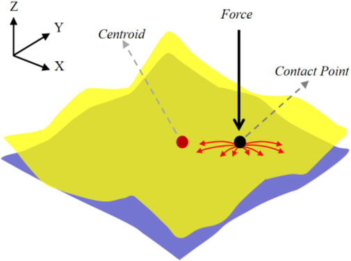
Figure 4. Single-point contact.

Figure 5

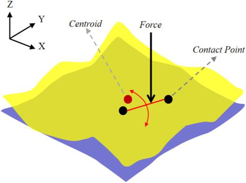
Figure 5. Two-point contact.

Figure 6

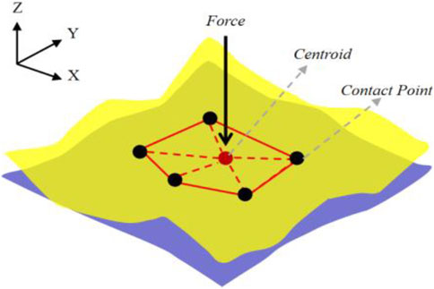
Figure 6. Satisfying force stability condition.

Figure 7

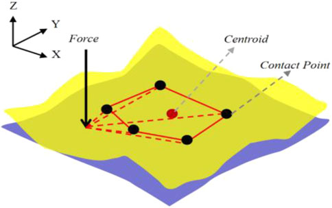
Figure 7. Not satisfying force stability condition.

The specific method to determine whether this condition is satisfied is as follows: assume the point of force $Force$ is located at a point $Q$ on the surface to be matched $S_2$. Project this point onto the convex hull formed by the contact points, with the projected point denoted as $Q^{\prime }$. If $Q^{\prime }$ lies within the convex hull of the contact points, the force stability condition is satisfied, as illustrated in Figure 6; otherwise, the force stability condition is not satisfied, as shown in Figure 7.

To address Constraint Condition 2, this study utilizes the minimum Euclidean distance from the point of force to the boundary of the convex hull as a penalty term, formulating the penalty expression as shown in Equation 6.

$penalty2=\left\{\begin{array}{l}0,Q^{\prime }\in CH\\ \min \left(dis\tan ces2\right),Q^{\prime }\notin CH\end{array}\right.(6)$

Here, $\min \left(dis\tan ces2\right)$ represents the minimum Euclidean distance from the point of force to all vertices of the convex hull formed by the contact points, denoted as $CH$. If $Q^{\prime }\in CH$, it indicates that $Q^{\prime }$ lies within the convex hull formed by the contact points, thereby satisfying the force stability requirement, resulting in $\text{penalty}2=0$. Otherwise, if $Q^{\prime }$ lies outside the convex hull, the force stability requirement is not satisfied, and $penalty2=\min \left(dis\tan ces2\right)$.

Finally, by incorporating the expressions of the above two constraints, this study employs the penalty function method to improve the optimization objective, transforming the multi-constraint optimization problem into an unconstrained optimization problem. The objective function of Equation 1 is redefined as Equation 7:

$F\left(T_k,R_k\right)=\min {\displaystyle \frac{1}{m}\sum _{i=1}^m}||R_k{P}_{i,k-1}+T_k-M_{i,k}||+{\displaystyle \sum _{i=1}^m}penalty1+{\displaystyle \sum _{i=1}^m}penalty2(7)$

3 Model solving based on improved particle swarm optimization algorithm

In the process of solving the surface matching model, the basic Particle Swarm Optimization (PSO) algorithm is prone to getting trapped in local optima. Moreover, the random generation of initial particle positions may lead to uneven distribution of particles. To address these issues, this study proposes an improved PSO algorithm for solving the surface matching model. In the solving process, $\alpha$, $\beta$, $\gamma$, $t_x$, $t_y$, $t_z$ are treated as six-dimensional variables, and the improved objective function from Section 2.2 is used as the fitness function.

To address the shortcomings of the basic Particle Swarm Optimization (PSO) algorithm in model solving, this study introduces improvements in the following aspects:

(1) To address the issue of uneven particle distribution caused by the random generation of initial particle positions in the Particle Swarm Optimization (PSO) algorithm, which may negatively affect population diversity (Kang et al., 2024; Xufan et al., 2021), this study employs the Spatial Pyramid Matching (SPM) with chaotic mapping to initialize the population. This approach ensures a uniform distribution of the initial population and enhances population diversity. The effectiveness diagram of population initialization based on the SPM chaotic map is shown in Figure 8. To deeply analyze the distribution of chaotic values across various ranges, this study has conducted statistics on the frequency of occurrence of midpoints within each chaotic value range and presented the statistical results in Figure 9. From Figures 8, 9, it is clearly observable that initializing the population using the Spatial Pyramid Matching (SPM) with chaotic mapping results in a well-distributed and uniform characteristic of the population in space. Therefore, this method can effectively overcome the potential randomness defects in the population generation process of the basic PSO algorithm, thereby enhancing population diversity.

(2) To address the issue of the Particle Swarm Optimization (PSO) algorithm being prone to local optima, this study proposes an adaptive adjustment strategy that dynamically adjusts the inertia weight using a hyperbolic tangent function. The approach is as follows: Initially, during the early stages of the search, a slower rate of decrease is employed to allow the particles sufficient time for global exploration, thereby reducing the risk of getting trapped in local optima. Subsequently, in the middle stages of the search, the rate of decrease is accelerated to enhance local search capabilities. Finally, as the search approaches its conclusion, the rate of change is reduced to ensure that the algorithm can focus effectively on local refinement.

(3) To enhance the global search capability of the Particle Swarm Optimization (PSO) algorithm, this study proposes an efficient and accurate hybrid strategy. This strategy integrates the Metropolis criterion from the Simulated Annealing algorithm (Yao et al., 2024) into the basic PSO, ensuring sufficient flexibility for broad exploration of potential solutions in the initial stages. As the temperature gradually decreases, the algorithm increasingly focuses on refining the solution to identify optimal regions.

Figure 8

Figure 8. Population initialization based on the spatial pyramid matching (SPM) with chaotic mapping.

Figure 9

Figure 9. Chaos value frequency statistics diagram.

The model solving process based on the improved Particle Swarm Optimization (PSO) algorithm is illustrated as follows:

Step 1: Initialize parameters, including population size $N$, the number of dimensions for the optimization variables $D$, maximum and minimum inertia weight coefficients ${\omega }_{\max }$ and ${\omega }_{\min }$, maximum and minimum social learning factors $c_{1\max }$ and $c_{1\min }$, maximum and minimum self-learning factors $c_{2\max }$ and $c_{2\min }$, maximum number of iterations $k_{\max }$, and the simulated annealing factor $\lambda$.

Step 2: Use the Spatial Pyramid Matching (SPM) with chaotic mapping to initialize the position and velocity of all particles in the population. The expression for the SPM chaotic mapping function is shown in Equation 8. Equations 9, 10 are used to transform the chaotic values into the search space of the population, thereby obtaining the new initial values for particle positions and velocities, denoted as ${X_i}^{\prime }$ and ${V_i}^{\prime }$.

$x\left(i+1\right)=\left\{\begin{array}{l}\mathit{mod}\left(\frac{x\left(i\right)}{\tau }+\mu \mathit{sin}\left(\pi x\left(i\right)\right)+r,1\right),0\le x\left(i\right)<\tau \\ \mathit{mod}\left(\frac{x\left(i\right)/\tau }{0.5-\tau }+\mu \mathit{sin}\left(\pi x\left(i\right)\right)+r,1\right),\tau \le x\left(i\right)<0.5\\ \mathit{mod}\left(\frac{\left(1-x\left(i\right)\right)/\tau }{0.5-\tau }+\mu \mathit{sin}\left(\pi \left(1-x\left(i\right)\right)\right)+r,1\right),0.5\le x\left(i\right)<1-\tau \\ \mathit{mod}\left(\frac{1-x\left(i\right)}{\tau }+\mu \mathit{sin}\left(\pi \left(1-x\left(i\right)\right)\right)+r,1\right),1-\tau \le x\left(i\right)<1\end{array}\right.(8)$

${X_i}^{\prime }=X_{\min }+X_i\left(X_{\max }-X_{\min }\right)(9)$

${V_i}^{\prime }=V_{\min }+V_i\left(V_{\max }-V_{\min }\right)(10)$

When $\tau \in \left(0,1\right)$ and $\in \left(0,1\right)$, the function is in a chaotic state. Here, $i=1,2,...,N$, where $N$ represents the population size; $r$ is a random number within the range [0,1] interval, and $X_{\min }$, $X_{\max }$, $V_{\min }$ and $V_{\max }$ represent the minimum and maximum values for particle position and velocity, respectively. In the text, $\tau =0.4$ and $\mu =0.3$.

Step 3: Calculate the fitness function value for each particle, and identify the individual and global optimal solutions based on these values. The initial temperature for simulated annealing is set according to Equation 12. In this study, the improved objective function presented in Section serves as the fitness function, defined as Equation 11:

$Fit=F\left(T_k,R_k\right)(11)$

$t\left(k\right)=\left\{\begin{array}{l}Fit\left(gbes{t}_{id}^k\right)/\log \left(5\right),k=1\\ t_0\left(k-1\right)\lambda ,k>1\end{array}\right.(12)$

Here, $t_0$ represents the initial temperature, $Fit\left(gbes{t}_{id}^k\right)$ denotes the fitness value of the global optimum, $\lambda$ is the simulated annealing coefficient, and $k$ is the current iteration number.

Step 4: Update the velocity of the particle swarm using Equation 13 and adjust the position of the particle swarm according to Equation 14. Equations 15–17 are used to adaptively adjust the inertia weight $\omega$ and learning factors $c_1$ and $c_2$.

$V_{id}^{k+1}=\omega \cdot V_{id}^k+c_1\cdot rand\cdot \left(pbes{t}_{id}^{k+1}-X_{id}^k\right)+c_2\cdot rand\cdot \left(gbes{t}_{id}^{k+1}-X_{id}^k\right)(13)$

$X_{id}^{k+1}=X_{id}^k+V_{id}^{k+1}(14)$

$\omega =\frac{{\omega }_{\max }+{\omega }_{\min }}{2}+\tanh \left(-4+8\times \frac{k_{\max }-k}{k_{\max }}\right)\frac{{\omega }_{\max }-{\omega }_{\min }}{2}(15)$

$c_1=c_{1\max }-\frac{\left(c_{1\max }-c_{1\min }\right)\times \left(k-1\right)}{k_{\max }-1}(16)$

$c_2=c_{2\max }-\frac{\left(c_{2\max }-c_{2\min }\right)\times \left(k-1\right)}{k_{\max }-1}(17)$

Here, $i=1,2,...,N$ , where N represents the population size; $d=1,2,...,D$, where $D$ denotes the dimensionality of the optimization variables; $rand$ is a random number between 0 and 1; $pbes{t}_{id}^k$ represents the individual best solution; $gbes{t}_{id}^k$ denotes the global best solution; ${\omega }_{\max }$ and ${\omega }_{\min }$ represent the maximum and minimum values of inertia weight, respectively; $c_1$ and $c_2$ represent the social learning factor and the self-learning factor, respectively; $c_{1\min }$, $c_{1\max }$, $c_{2\min }$ and $c_{2\max }$ denote the minimum and maximum values of the social and self-learning factors; $k_{\max }$ represents the maximum number of iterations; $k$ denotes the current iteration number. In the equations. In the equations, $N=50$, $D=6$, ${\omega }_{\max }=0.9$, ${\omega }_{\min }=0.4$, $c_{1\min }=1.25$, $c_{1\max }=2.5$, $c_{2\min }=1.25$, $c_{2\max }=2.5$, $k_{\max }=50$.

Step 5: Calculate the fitness value of each particle after the updates in the previous step, and determine whether it is better than the previous generation. If the current position of an updated particle shows a higher fitness than its historical best position, update the particle’s historical best position record; otherwise, accept the position with a certain probability. After evaluating all particles, compare and update the global best value for the entire swarm.

Step 6: According to the Metropolis criterion, calculate the probability $p_i\left(k\right)$ of accepting the new solution. The calculation formula is as Equation 18.

$p_i\left(k\right)=\left\{\begin{array}{l}1,Fi{t}_i\left(k\right)\ge Fi{t}_k\\ \exp \left(-\frac{Fi{t}_i\left(k\right)-Fi{t}_k}{t\left(k\right)}\right),Fi{t}_i\left(k\right)<Fi{t}_k\end{array}\right.(18)$

Here, $Fi{t}_i\left(k\right)$ represents the fitness value of particle $i$ in $k$-th iteration; $Fi{t}_k$ denotes the fitness value of the current global best position in the swarm; $t\left(k\right)$ indicates the temperature at the $k$-th iteration.

Step 7: Compare the probability $p_i\left(k\right)$ with $rand\left(0,1\right)$ to determine whether the new solution generated by particle $i$ should replace the global best solution for simulated annealing. If $Fi{t}_i\left(k\right)<Fi{t}_k$, then the new solution is accepted as the current solution; if $\exp \left(-\frac{Fi{t}_i\left(k\right)-Fi{t}_k}{t\left(k\right)}\right)$ greater than a random number between 0 and 1, the new solution is still accepted as the current solution. If so, proceed with the cooling process and update the temperature; otherwise, return to Step 4.

Step 8: Check whether the termination condition for iterations is met. If not, return to Step 4 to continue with the next iteration; otherwise, output the current best particle, which is the optimal solution for the parameter vector $\left(\alpha ,\beta ,\gamma ,t_x,t_y,t_z\right)$.

4 Example verification

4.1 Verification case

To validate the effectiveness of the proposed method, a precision machining vibrating disk is selected as the verification object. This disk primarily comprises components such as the hopper and chassis, where the quality of assembly has a direct impact on the accuracy of precision products. Within the vibrating disk, the components are aligned and matched through interfacing surfaces. The assembly configuration is illustrated in Figure 10. This study focuses on two critical components, Part1 and Part 2, both of which have rotational structures with annular planar contact interfaces.

Figure 10

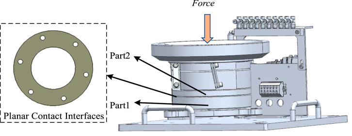
Figure 10. Assembly drawing of the vibrating disk for net area processing.

4.2 Algorithm performance test

To verify the performance of the improved particle swarm optimization algorithm proposed in this study, four test functions were employed to evaluate both the proposed algorithm and the basic particle swarm optimization algorithm. The specific expressions of the test functions and the settings for the search spaces are detailed in Table 1. Simulations were conducted in the MATLAB 2022a environment, with the population size of particles uniformly set to 50 and the maximum number of iterations set to 1,000. For the other parameters of the improved particle swarm optimization algorithm, the same settings as described in Section 3 of this study were adopted. For the basic particle swarm optimization algorithm, a linear inertia weight factor, as shown in Equation 19, is used, with the other parameters set as follows: ${\omega }_{\max }=0.9$, ${\omega }_{\min }=0.4$, $c_2=1.7$, $c_1=1.3$.

$\omega ={\omega }_{\max }-\frac{\left({\omega }_{\max }-{\omega }_{\min }\right)\times \left(k-1\right)}{k_{\max }-1}(19)$

Table 1

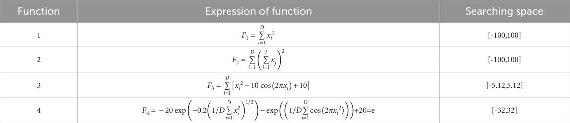
Table 1. Test Function information.

The optimal values obtained from testing the improved particle swarm optimization algorithm and the basic particle swarm optimization algorithm using the four functions in Table 1 are shown in Table 2.

Table 2

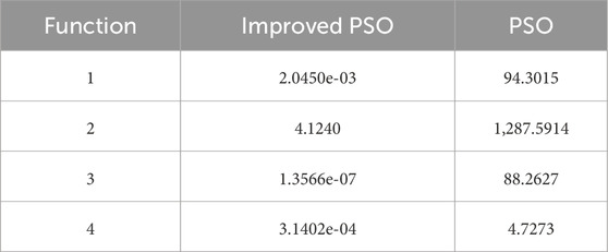
Table 2. The best optimal value of objective function.

As can be seen from Table 2, the optimal values of the objective functions for the improved particle swarm optimization algorithm are significantly smaller than those for the basic particle swarm optimization algorithm. Therefore, the algorithm proposed in this paper demonstrates higher accuracy.

To visually compare the difference in accuracy between the two algorithms, iterative curve graphs of the algorithms tested using different test functions are plotted, as shown in Figure 11.

Figure 11

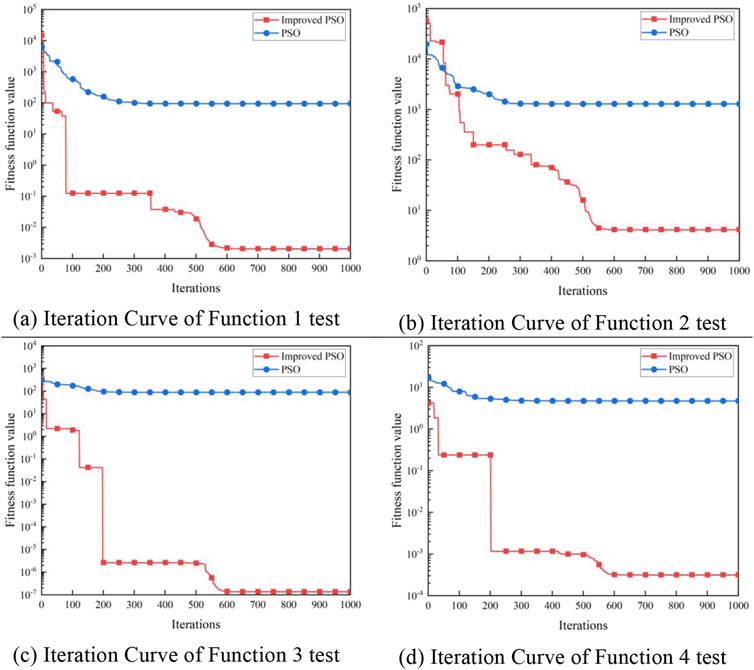
Figure 11. Algorithm Iteration Curves. (A) Iteration Curve of Function one test. (B) Iteration Curve of Function two test. (C) Iteration Curve of Function 3 test. (D) Iteration Curve of Function four test.

Observing Figure 11, it can be seen that although the accuracy of the improved particle swarm optimization algorithm in (a), (b), and (c) is not as high as that of the basic particle swarm optimization algorithm at the initial iterations, the accuracy of (a) and (c) exceeds that of the basic particle swarm optimization algorithm before 50 iterations, and (b) does so before 100 iterations. In (c), the accuracy of the improved particle swarm optimization algorithm is consistently higher than that of the basic particle swarm optimization algorithm, which verifies that the algorithm proposed in this study has certain advantages in terms of accuracy. However, the convergence speed of the basic particle swarm optimization algorithm is faster than that of the algorithm proposed in this study, because most particles in the population have converged to local optima. Nevertheless, the algorithm proposed in this study can significantly enhance the ability to escape from local optima, and it can continue to update the global optimum in the middle to late stages of iterations, thereby improving the accuracy of the search results. In summary, the improved particle swarm optimization algorithm presented in this study has certain advantages.

4.3 Experimental verification

To validate the effectiveness of the proposed method and the robustness of the improved particle swarm algorithm, we sampled 1,152 3D point cloud data points from the lower surface of Part 2, denoted as $P=\left\{P_1,P_2,\cdots ,P_{1152}\right\}$, forming the source point set. After triangular meshing, the upper surface of Part 1 consisted of 1,279 triangular meshes, denoted as $M=\left\{M_1,M_2,\cdots ,M_{1279}\right\}$, which served as inputs to the algorithm. By searching for the nearest points from the source point cloud to the triangular meshes, we identified the closest points as the target point set $P^{\prime }$, represented by $P^{\prime }=\left\{P_1^{\prime },P_2^{\prime },\cdots ,P_{1152}^{\prime }\right\}$. Thus, each point in the source point set corresponds to the nearest point in the target point set, forming a nearest-distance pairing. Through iterative computation, the algorithm derives an optimal transformation matrix, output as a parameter vector $\left(\alpha ,\beta ,\gamma ,t_x,t_y,t_z\right)$.

For comparative analysis of assembly error, three experimental groups were set up: the first group used the standard particle swarm algorithm to solve for a single fixed pose model; the second group employed the improved particle swarm algorithm for the same single fixed pose model; and the third group applied the improved particle swarm algorithm to solve for multiple fixed pose models.

Through the above three experiments, the transformation parameters for each experiment were obtained, as shown in Table 3.

Table 3

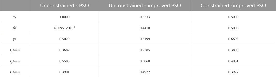
Table 3. Transformation parameters obtained under three different conditions.

The transformation parameters in Table 3 are visualized in Figure 12. For parameter α, the third experimental group exhibits the largest deviation from the first group, with an error of 0.5000. For parameter β, the value in the first group is nearly zero, showing a substantial discrepancy compared to the other two groups. For parameter γ, the first and second groups are relatively close, while the third group shows deviations of 0.1664 and 0.1194 from the first and second groups, respectively. For parameter $t_x$, the values of the first and third groups are comparable, with the second group differing by 0.0118 and 0.1515 from the other two groups. For parameter $t_y$, the first and second groups exhibit the greatest difference, with an error of 0.2523. Finally, for parameter $t_z$, the second group achieves the highest value.

Figure 12

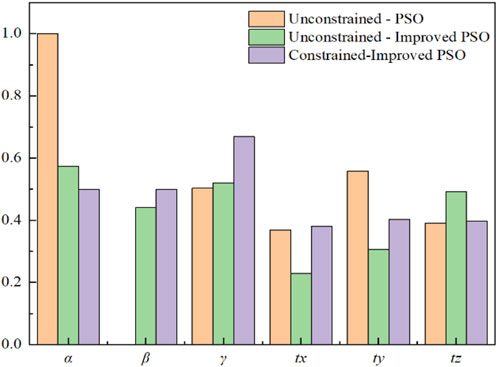
Figure 12. Comparison of transformation parameters.

Figure 13 presents the changes in optimal fitness values over iterations for the three experimental conditions. Upon completing the iterations, the target fitness values under the three different conditions were 1.5375 $\times {10}^{-3}$ mm, 1.0914 $\times {10}^{-3}$ mm and 2.4345 $\times {10}^{-3}$ mm, respectively. The results demonstrate that the improved particle swarm algorithm achieved 29% higher accuracy than the basic particle swarm algorithm when solving the unconstrained fixed pose model, validating the robustness of the improved algorithm. When the improved particle swarm algorithm was applied to solve the multiple constrained fixed pose model, the target fitness value was 1.6 times that of the unconstrained model solved with the basic algorithm, and 2.2 times that of the constrained fixed pose model solved with the basic algorithm. The lower target fitness value observed for the multiple constrained fixed pose model using the improved particle swarm algorithm, in comparison with the other two cases, will be further discussed with reference to Table 4 in the subsequent analysis.

In Figure 13, it can be observed that the fitness function value of the improved particle swarm algorithm without constraints is higher than that of the basic particle swarm algorithm at the initial stage. However, in the final stage of the search, the fitness function value of the improved particle swarm algorithm is lower than that of the basic algorithm, indicating higher accuracy. This validates the effectiveness of the improvement strategy proposed in this paper.

Figure 13

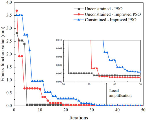
Figure 13. Algorithm iteration curves under three different conditions.

Table 4 outlines the interference conditions across three scenarios, detailing both the number of interference points and their percentage relative to the total points. To assess the validity of the non-interference constraint proposed in this study, we examined the frequency of interference points in each experimental group. The statistical is as follows: by calculating the signed distance between the point cloud and the triangular grid, if the signed distance is positive, it means that the point is “above” relative to the grid, that is, the point is an interference point; On the contrary, if the calculated signed distance is negative, it means that the point is “blow” relative to the grid, that is, it is not an interference point. The result shows that the first experiment exhibited interference in 34.64% of the points, while the second experiment showed interference in 43.66% of the points. Notably, the third experiment displayed no interference. These results confirm the reasonableness of imposing a non-interference constraint between the two surfaces, as a sole focus on minimizing the distance does not adequately capture the realities of the assembly process. Furthermore, they support the appropriateness of the third experiment’s higher target function value at the conclusion of the iteration process.

Table 4

Table 4. Interference points under three different conditions.

Upon completion of the surface matching, the final contact points between the two surfaces were computed. The coordinates of these contact points, obtained under the three different conditions, are presented in Tables 5–7, respectively.

Table 5

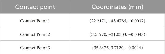
Table 5. Contact point coordinates obtained using unconstrained PSO.

Table 6

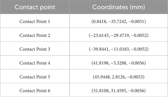
Table 6. Contact point coordinates obtained using unconstrained - improved PSO (mm).

Table 7

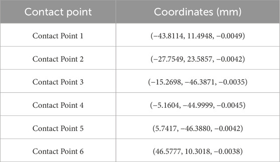
Table 7. Contact point coordinates obtained using multiple constrained improved PSO (mm).

In the assembly positioning results obtained under the three different conditions, the convex hull formed by the contact points is visualized in Figures 14–16, respectively. Given that the hopper exerts pressure on the lower components when loaded, the position of the force in these figures represents the location of the equivalent force. The results demonstrate that in Figure 14, the force projection point lies outside the convex hull formed by the contact points, indicating non-compliance with stability requirements. Conversely, in Figures 15, 16, the force projection points are contained within the convex hull, thereby meeting stability requirements. These findings confirm the necessity of incorporating force stability considerations in the proposed method.

Figure 14

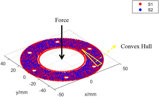
Figure 14. Assembly positioning results using unconstrained PSO.

Figure 15

Figure 15. Assembly positioning results using unconstrained improved PSO.

Figure 16

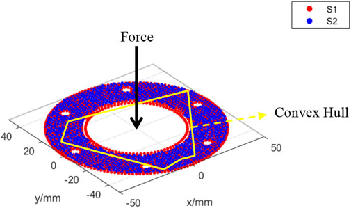
Figure 16. Assembly positioning results using multiple constraints with improved PSO.

5 Conclusion

This study presents a precision assembly error analysis method utilizing multi-constrained surface matching to capture the complexities inherent more accurately in real-world precision assembly processes. In constructing the assembly positioning model, this approach incorporates non-interference and force stability constraints to provide a more authentic and accurate representation of surface matching. For model optimization, SPM chaotic mapping was utilized for population initialization to enhance diversity, while a hyperbolic tangent function was applied as a nonlinear control strategy to dynamically adjust inertia weight. Additionally, a simulated annealing mechanism was integrated into the particle swarm optimization (PSO) algorithm to overcome the tendency of conventional PSO to become trapped in local optima. The proposed method was validated through an assembly experiment involving a precision machining vibrating disk. Results from three experimental groups indicate that the improved algorithm not only offers superior accuracy compared to the original PSO but also more accurately reflects the actual contact conditions, aligning closely with the practical assembly process. Future research could further explore the effects of force magnitude on the positioning of contact points between two mating surfaces with inherent tolerances in precision assembly, as well as the impact of deformation caused by assembly forces on assembly errors. Taking into account the uncertainty in experimental measurements and the mechanism of how this uncertainty propagates through the analysis process, further research is also needed to establish a relationship between predicted assembly errors and experimentally measured errors.

Data availability statement

The original contributions presented in the study are included in the article/supplementary material, further inquiries can be directed to the corresponding author.

Author contributions

WT: Conceptualization, Methodology, Writing–original draft. TY: Data curation, Methodology, Writing–original draft. JS: Writing–original draft, Writing–review and editing. YL: Writing–original draft.

Funding

The author(s) declare that financial support was received for the research, authorship, and/or publication of this article. This work was supported by the National Natural Science Foundation of China under Grant 52105559, the Aviation Science Foundation under Grant 2022Z050111001, the Xi’an Science and Technology program under Grant 23GXFW0022, the Natural Science Foundation of Shaanxi Province under Grant 2021JQ-680, the Key Research and Development Program of Shaanxi under Grant 2024GX-YBXM-278 and the Scientific Research Foundation for Doctor of Xi’an Polytechnic University under Grant BS201909.

Conflict of interest

The authors declare that the research was conducted in the absence of any commercial or financial relationships that could be construed as a potential conflict of interest.

Generative AI statement

The author(s) declare that no Generative AI was used in the creation of this manuscript.

Publisher’s note

All claims expressed in this article are solely those of the authors and do not necessarily represent those of their affiliated organizations, or those of the publisher, the editors and the reviewers. Any product that may be evaluated in this article, or claim that may be made by its manufacturer, is not guaranteed or endorsed by the publisher.

References

Chauhan, S., Vashishtha, G., Zimroz, R., Kumar, R., and Kumar Gupta, M. (2024). Optimal filter design using mountain gazelle optimizer driven by novel sparsity index and its application to fault diagnosis. Appl. Acoust. 225, 225 110200–110200. doi:10.1016/j.apacoust.2024.110200

CrossRef Full Text | Google Scholar

Chen, Q., Feng, D., Zheng, W., and Feng, X. (2023). An efficient point-set registration algorithm with dual terms based on total least squares. Pattern Recognit., 134.

Google Scholar

Cheng, Y., Chu, H., Li, Y., Tang, Y., Luo, Z., and Li, S. (2024). A hybrid improved SAC-IA with a KD-ICP algorithm for local point cloud alignment optimization. Photonics 11 (7), 635. doi:10.3390/photonics11070635

CrossRef Full Text | Google Scholar

Guokai, Z., Chunmei, L., and Yuexi, Z. (2022). Point cloud registration method based on Particle Swarm Optimization algorithm and improved ICP. J. Phys. Conf. Ser. 2395 (1), 012078. doi:10.1088/1742-6596/2395/1/012078

CrossRef Full Text | Google Scholar

Han, J., Yin, P., He, Y., and Gu, F. (2016). Enhanced ICP for the registration of large-scale 3D environment models: an experimental study. Sensors 16 (2), 228. doi:10.3390/s16020228

PubMed Abstract | CrossRef Full Text | Google Scholar

Jingyu, S., Yadong, G., Jibin, Z., Zhang, H., and Jin, L. (2023). Matching based on variance minimization of component distances using edges of free-form surfaces. Pattern Recognit. 143, 109729. doi:10.1016/j.patcog.2023.109729

CrossRef Full Text | Google Scholar

Kang, L., Lai, Y., Wang, J., and Cao, W. (2024). A Pacesetter-Lévy multi-objective particle swarm optimization with Arnold Chaotic Map with opposition-based learning. Inf. Sci. 678, 121048. doi:10.1016/j.ins.2024.121048

CrossRef Full Text | Google Scholar

Lin, T., Ailing, Z., Sha, L., Minghua, D., and Pengfei, L. (2022). Design and simulation of logistics network model based on particle swarm optimization algorithm. Comput. Intell. Neurosci. 22, 1862911.

Google Scholar

Liu, J. H., Xia, H. X., Gong, H., Liu, S. L., Zhuang, C. B., and Ao, X. H. (2023). Connotation, technical system and development trend of precision assembly. J. Mech. Eng. 59 (20), 436–450.

Google Scholar

Pottmann, H., Huang, Q. X., Yang, Y. L., and Hu, S. M. (2006). Geometry and convergence analysis of algorithms for registration of 3D shapes. Int. J. Comput. Vis. 67, 277–296. doi:10.1007/s11263-006-5167-2

CrossRef Full Text | Google Scholar

Schleich, B., and Wartzack, S. (2018). Novel approaches for the assembly simulation of rigid Skin Model Shapes in tolerance analysis. Computer-Aided Des. 101, 1–11. doi:10.1016/j.cad.2018.04.002

CrossRef Full Text | Google Scholar

Sun, Q., Zhao, B., Liu, X., Mu, X., and Zhang, Y. (2019). Assembling deviation estimation based on the real mating status of assembly. Computer-Aided Des. 115, 244–255. doi:10.1016/j.cad.2019.06.001

CrossRef Full Text | Google Scholar

Tian, Y., Yue, X., and Zhu, J. (2023). Coarse–fine registration of point cloud based on new improved whale optimization algorithm and iterative closest point algorithm. Symmetry 15 (12), 2128. doi:10.3390/sym15122128

CrossRef Full Text | Google Scholar

Vashishtha, G., Chauhan, S., Sehri, M., Zimroz, R., Dumond, P., Kumar, R., et al. (2025b). A roadmap to fault diagnosis of industrial machines via machine learning: a brief review. Measurement 242 (PD), 116216. doi:10.1016/j.measurement.2024.116216

CrossRef Full Text | Google Scholar

Vashishtha, G., Chauhan, S., Zimroz, R., Kumar, R., and Kumar Gupta, M. (2025a). Optimization of spectral kurtosis-based filtering through flow direction algorithm for early fault detection. Measurement 241, 115737. doi:10.1016/j.measurement.2024.115737

CrossRef Full Text | Google Scholar

Wang, D. S., Tan, D. P., and Liu, L. (2018). Particle swarm optimization algorithm:an overview. Soft Comput. 22, 387–408. doi:10.1007/s00500-016-2474-6

CrossRef Full Text | Google Scholar

Wen, F. M., Shen, L. W., and Jin, Q. P. (2009). Automatic point clouds registration based on the method of least squares. Key Eng. Mater. 419-420 (429-420), 305–308. doi:10.4028/www.scientific.net/kem.419-420.305

CrossRef Full Text | Google Scholar

Wu, P., Li, W., and Yan, M. (2020). 3D scene reconstruction based on improved ICP algorithm. Microprocess. Microsystems 75, 103064. doi:10.1016/j.micpro.2020.103064

CrossRef Full Text | Google Scholar

Wv, W., Xiaokai, M., Wei, Z., Jiang, H., Ji, X., Sun, Q., et al. (2024). A novel prediction method for assembly accuracy of rudder systems considering clearance factors. Int. J. Adv. Manuf. Technol. 131 (9-10), 4621–4634. doi:10.1007/s00170-024-13264-w

CrossRef Full Text | Google Scholar

Xufan, D., Kui, L., Dan, S., Zhu, Z., and Zhang, Y. (2021). Optimal economic dispatch of microgrid based on chaos map adaptive annealing particle swarm optimization algorithm. J. Phys. Conf. Ser. 1871 (1), 012004. doi:10.1088/1742-6596/1871/1/012004

CrossRef Full Text | Google Scholar

Yan, X., and Ballu, A. (2018). Tolerance analysis using skin model shapes and linear complementarity conditions. J. Manuf. Syst. 48, 140–156. doi:10.1016/j.jmsy.2018.07.005

CrossRef Full Text | Google Scholar

Yao, J., Li, Y., Yu, X., Liu, Y., Sun, S., and Yan, Y. (2024). Acceleration harmonic identification for an electro-hydraulic shaking table based on the Simulated Annealing-Particle Swarm Optimization algorithm. J. Vib. Control 30 (1-2), 193–204. doi:10.1177/10775463221143409

CrossRef Full Text | Google Scholar

Yi, Y., Zhang, A., Liu, x, Jiang, D., Lu, Y., and Wu, B. (2024). Digital twin-driven assembly accuracy prediction method for high performance precision assembly of complex products. Adv. Eng. Inf. 61, 102495-. doi:10.1016/j.aei.2024.102495

CrossRef Full Text | Google Scholar

Yongsheng, L., Panru, H., Zhibo, X., Chen, Y., and Tan, J. (2023). Tooth surface registration of spiral bevel gear based on improved genetic algorithm. J. Phys. Conf. Ser. 2562 (1), 012020. doi:10.1088/1742-6596/2562/1/012020

CrossRef Full Text | Google Scholar

Zhang, K., Gao, K., and Zhang, H. (2007). A minimum zone method for evaluating flatness errors based on PSO algorithm[C]. Shanghai, P. R.China: Shanghai Institute of Technology. Zhejiang Wanli University, China; Suzhou Mingzhi Foundry Equipment Co., Ltd.

Google Scholar

Zhang, Q., Zhang, Z., Jin, X., Zeng, W., Lou, S., Jiang, X., et al. (2019). Entropy-based method for evaluating spatial distribution of form errors for precision assembly. Precis. Eng. 60, 374–382. doi:10.1016/j.precisioneng.2019.07.020

CrossRef Full Text | Google Scholar

Zhang, Q. S., Jin, X., Zhang, Z. Q., Zhang, Z. J., and Shang, K. (2018). Assembly method based on constrained surface registration. J. Mech. Eng. 54 (11), 70–76. doi:10.3901/jme.2018.011.070

CrossRef Full Text | Google Scholar

Zhang, S., Wang, H., Wang, C., Wang, Y., and Yang, Z. (2024). An improved RANSAC-ICP method for registration of SLAM and UAV-LiDAR point cloud at plot scale. Forests 15 (6), 893. doi:10.3390/f15060893

CrossRef Full Text | Google Scholar

Zhang, T. Y. (2016). Assembly accuracy prediction and control for precision mechanical system[D]. China: Beijing Institute of Technology.

Google Scholar