 Fei Song
 Kevin Shi
 Ke Li
Ke Li
94% of researchers rate our articles as excellent or good
Learn more about the work of our research integrity team to safeguard the quality of each article we publish.
Find out more
ORIGINAL RESEARCH article
Front. Mech. Eng., 12 June 2024
Sec. Solid and Structural Mechanics
Volume 10 - 2024 | https://doi.org/10.3389/fmech.2024.1410360
This article is part of the Research TopicHybrid Modeling - Blending Physics with DataView all 5 articles
In this study, a Bayesian data assimilation method that fuses physics with motion sensor data is demonstrated to infer the dynamic states at points of interest on the bottomhole assembly (BHA) with proper uncertainty quantification. A 4.75 inch-LWD (Logging-while-drilling) tool has been used as a use case, where the dynamic states at the formation evaluation sensor can be predicted in real time with the measurements at the motion sensor as the required inputs. This was achieved with a developed transfer function that utilizes unscented Kalman filtering technique. The robustness of the transfer function was evaluated with synthetic data obtained from finite element analysis (FEA) simulations for various BHA configurations and drilling conditions. It was found that the prediction by the transfer function agrees favorably well with the true states of motion at the formation evaluation sensor. Specifically, using the developed transfer function can help reduce the relative errors for the motion trajectories at the formation evaluation sensor by a factor of 3, and can significantly enhance measurement quality risk classification. The developed transfer function method was further assessed with experimental roll test data, which is considered as close to drilling conditions. The prediction by the transfer function was found consistently close to the ground truth in the presence of backward whirl. The developed modeling method can potentially have broader impacts by enabling fit-for-basin virtual V&V (Verification and Validation) to accelerate LWD tool development, or enabling future drilling optimization.
Logging-while-drilling (LWD) is a general term to describe systems and techniques for gathering downhole data while drilling without the requirement to remove drill pipe from the well (Tollefsen et al., 2007). LWD offers similar functionality as wireline logging with differences in data quality, resolution, and/or coverage (Simpson, 2017). LWD tools are basically large drill collars instrumented with advanced formation measurement device and sensors, which are often contained in the bottomhole assembly (BHA) located at the lowest section of the drillstring (Chen et al., 2019a; Hegdea et al., 2019), as shown in Figure 1. The formation evaluation (FE) sensor is the core device on the LWD tool, which is responsible for measuring porosity, resistivity, acoustic waveform, and others. LWD transmits logging measurements at regular intervals while drilling takes place. Data is transmitted to the surface through the mud column (also known as mud pulse of mud telemetry) in a real-time manner (Shi et al., 2022; Li and Xu, 2023). Drillers and operators can consume LWD information immediately to define well placement and predict drilling hazards. Use of real-time logging information provided by LWD enables more intelligent drilling, and stronger, more successful wells both onshore and offshore.
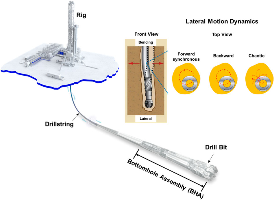
Figure 1. Illustration of BHA lateral motion dynamics in a drillstring.
The performance and health of LWD tools can be significantly impacted by drilling dynamics of the BHA. Considerable effort has been made to understand complex dynamics of beam-like structures or drillstrings by means of numerical modeling or experimental verification (Jansen, 1992; Pany et al., 2001; Pany and Rao, 2002; Pany and Rao, 2004; Chen et al., 2015; Vamsi et al., 2021; Pany, 2022; Song et al., 2022; Pany, 2023; Song et al., 2023). With drilling dynamics becoming increasingly harsh, BHA whirl is one of the undesired motions the tool can face during drilling operations, where the BHA follows an eccentric rotation about a point along the wellbore other than the geometric center (Zhao et al., 2017; Kapitaniak et al., 2018). BHA whirl could be forward or backward whirl (see Figure 1). Forward whirl is when the BHA robs the formation along the same part of the collar as the drill string rotates. The BHA still rotates in the same direction as the drill string in forward whirl. Backward whirl is formed in which the increased friction leads to increased torque on the BHA and causes the BHA to rotate in the opposite direction of the rotation of the drillstring. Backward whirl is an extremely violent phenomenon affecting rotary drilling assemblies. Traction is produced at contact points between the drilling assembly and the borehole wall, which can force the drilling assembly into rolling (rather than sliding) contact with the hole and a complex motion resulting in dramatically increased loading frequency and multiple borehole impacts (Wang et al., 2021; Song et al., 2022). Whirl-induced lateral motions could be one of the major concerns for measurement quality for LWD tools. For example, parasitic motion that causes a plethora of distortions to the echo train, at times manifesting as erratic noise or a complete loss of cohesion has been a measurement quality concern for LWD tools (Coman et al., 2018; Haji et al., 2020; Hursan et al., 2022). Modern LWD tools are commonly equipped with advanced motion sensors that can provide the amounts of observed data to partially describe the dynamic states of the BHA; however, these sensors can be installed only at discrete and limited locations along the LWD tools due to various constraints. If the sensor measurements are simply taken as the dynamic states at locations away from the sensors, risks associated with tremendous uncertainty can be present in decision making. The farther away from the sensors, the more uncertain the dynamic states could become. Therefore, robust inference of dynamic states at the formation evaluation sensor based on available motion sensor measurements is crucial for risk flagging and quality assurance of LWD answer products.
A variety of methods have been reported to reduce errors in simulation and prediction models during last 10 decades. Especially in the current big-data era, the amounts of observed data are rapidly growing due to the evolving measurement techniques and hardware improvement. Data assimilation (DA) is the methodology whereby observational data are combined with output from a first-principle model to optimally estimate the evolving state and/or parameters of the system (Wang et al., 2000; Wikle and Berliner, 2007; Schweidtmann et al., 2024). DA typically involves a sequential time-stepping procedure, where a previous model forecast is compared with newly received observations, the model state is then updated to reflect the observations, a new forecast is initiated, and so on. DA can reduce overall uncertainty by considering the uncertainties of the inputs, observations, and updating variables promptly, which is better than what could be obtained using just the data or the models alone since it is often challenging for a model to cover complete physics of real world, and sensor data are usually subjected to noises. DA for state or parameter estimation is commonly achieved through Bayesian inference, Kalman filtering or its variants, or Particle filtering (Wikle and Berliner, 2007; Shao et al., 2023). DA has found pilot applications in mechanical systems. To name a few, Hsu et al. (2006) implemented a sequential method, in which analyzed wave spectra and significant wave fields were assimilated by optimal interpolation, then the analyzed values were used to reconstruct the wave spectrum. Rubio et al. (2021) proposed a real-time data assimilation and control on mechanical systems under uncertainties. Hastermann et al. (2021) proposed data assimilation algorithms to estimate the states of a dynamical system using partial and noisy observations with modifications to the standard ensemble Kalman filter. Mohsan et al. (2024) implemented different data assimilation schemes such as the ensemble Kalman filter, ensemble smoother and ensemble smoother with multiple data assimilation in a hydromechanical slope stability analysis. This study seeks to leverage and extend the DA applications to help discover the drilling dynamics states at the formation evaluation sensor of the LWD tool with discrete motion sensor measurements.
In this paper, a UKF (Unscented Kalman Filter)-based data assimilation framework is presented to enable real-time prediction of the dynamic states at the formation evaluation sensor with the motion sensor data as the required inputs, along with appropriate uncertainty quantification. The remaining of the paper is organized as follows. Problem formulation and data assimilation methodology are first introduced, followed by a use case study on a 4.75 inch-LWD tool. The detailed study includes FEA-based multi-fidelity modeling, fusion of the underlying dynamic principles with motion sensor data, and model verification and validation (V&V) with synthetic data obtained from FEA and real data collected from a full-scale roll test system. The paper is finally closed with Conclusions based on the findings from this study.
A typical LWD tool that has 4.75-inch outer diameter (OD) and comprises outside collar and internal chassis is shown in Figure 2. There is one motion sensor mounted on the chassis, whereas the formation evaluation sensor is 8 inches away from the motion sensor. The LWD tool connects with the rest of the drillstring through crossovers. One could expect that the motion trajectories collected at the motion sensor could differ from the true dynamic states at the formation evaluation sensor when the BHA is subjected to whirl during drilling. The objective of this study is to develop a “transfer function (TrF)” that can, in a real-time manner, map the states measured at the motion sensor (illustrated with blue ellipse) to describe the true states at the formation evaluation sensor (depicted with green ellipse) with appropriate uncertainty quantification (illustrated with white ellipse that compasses the green ellipse; Refer to Figures 2, 3).
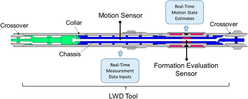
Figure 2. Schematic of a typical LWD tool with motion sensor and formation evaluation sensor.
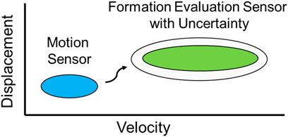
Figure 3. Schematic of transfer function concept for the LWD tool.
A drillstring is a long and slender assembly comprising various tubulars and drilling tools with complex geometry, which experiences complex environmental loads such as torque and drag, gravity, wellbore contact, friction, and dynamic inertia force caused by rotation. To consider the influences of these factors, a multi-fidelity modeling approach based on transient FEA is proposed.
At the drillstring level, a three-dimensional (3D) beam type of model is used to predict the dynamic responses of drillstring/BHA in a wellbore. The model is based on the finite element method (Argyris et al., 1979), where the drillstring is discretized into beam elements and each node has six degrees of freedom, including three translations and three rotations. This enables the model to predict complex motions of the drillstring in 3D space. Drillstring components from bit to surface are modeled in detail to describe the collar outside diameter variation and contact interactions with wellbore. Extensive laboratory cutting tests were conducted with various cutter shapes, formation types, and confining pressures. The learnings from the cutting tests were applied in the model to capture the bit-rock interaction, from which bit behaviors, such as torque, weight, depth of cut, and dynamics excitation, can be accurately computed. Coupling the bit and drillstring mechanics model enables the simulation of dynamic responses of the drillstring with greater confidence. The dynamics equilibrium equation is solved step by step to provide the time history of dynamics variables (i.e., accelerations and rotation speed) at each node of drillstring. The nonlinear coupling between bending and torsional vibrations could greatly affect the dynamic behavior of the drillstring, and the nonlinear coupling between torsional and bending DOF is thus considered in the FEA formulations, where a bending-torsion coupling term is presented in the governing equation. The robust implicit FEA engine enables the simulation of large deformation of tubulars under the confinement of the wellbore (Chen et al., 2019b; Chen et al., 2021). The transient dynamics model simulates the rotation of the drillstring and enables the drillstring to move freely inside the wellbore. There is no assumption made on the external force and contact location of the drillstring. The system transient response can be governed by the dynamics equilibrium equation as follows:
where
The limitation of the beam type model is that it captures collar sections by using their inner diameters (IDs) and outer diameters (ODs). However, it cannot describe the collar-chassis contact interactions, since the inside chassis is neglected. To consider the dynamic interaction between the collar and chassis, a 3D solid FEA model that can describe the detailed geometry of the LWD tool and sliding contact between the collar and chassis is required. Such high-fidelity FEA model to describe backward whirl of the LWD tool is implemented with commercially available explicit dynamics solver ANSYS LS-Dyna (Song et al., 2022). It should be noticed that load-carrying parts of the LWD tool such as collar and chassis are typically made of steels with high strength and good ductility having a minimum yield strength of 100ksi and elongation of around 20%. Considering structural integrity’s requirement during drilling, the drillstring is generally designed and operated within linear elastic region of its material to avoid global yield. Therefore, linear elastic material model is considered for the parts made of typical steels with Young’s modulus of 29,000 ksi, and Poisson’s ratio of 0.3 in the simulation. Geometric nonlinearity due to large deformation, if any, is considered in FEA. Coulomb friction with a coefficient of friction 0.1 is assumed for sliding contact interactions between the collar and chassis, because parts are well lubricated during assembling.
The FEA assembly model is meshed with 3D 4-node tetrahedral and 8-node hexahedral elements defined with “*SECTION_SOLID” card in ANSYS LS-Dyna. Figure 4 shows the meshes of the FEA model in ANSYS LS-Dyna. Sufficient refinement of elements needs to be considered especially in the areas of interest such as the locations where sensor outputs are requested. The meshes on the contact faces between the parts need also be refined with high quality such that the contacts can be detected appropriately, and risk of element distortion can be mitigated. Mesh sensitivity study was conducted: it was found that the variation of the displacements at the locations of interest were within 3% with the number of nodes increased from 823,926 to 1,516,213, which suggested a converged solution. 2.5e-7 second is determined as the minimum stable timestep in the Explicit dynamics simulation. In our previous publication, the tool model based on ANSYS LS-Dyna has shown promising results compared to experimental roll test data (Song et al., 2022).
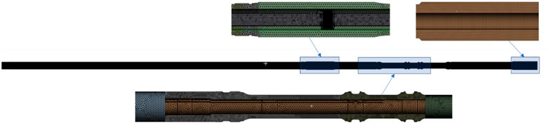
Figure 4. Mesh of the tool-level FEA model.
During drilling, the displacements could vary along the length of the drillstring due to dynamics and interaction between the drillstring and wellbore. The lateral displacements (
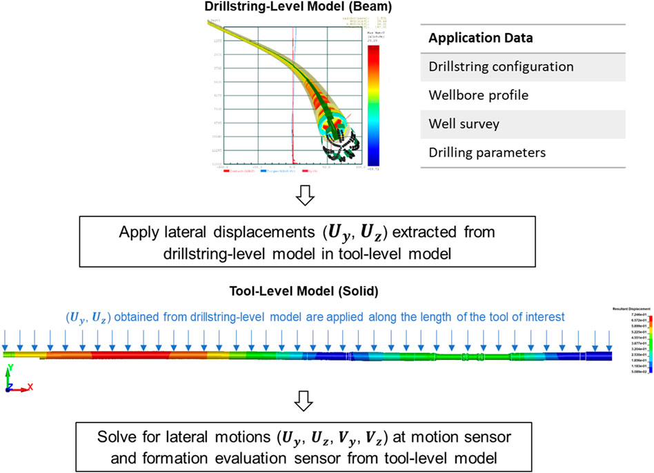
Figure 5. Multi-fidelity FEA modeling workflow.
Based on the multi-fidelity modeling approach described in Section 3.1, sufficient simulations can be executed offline, knowing these simulations are computationally expensive. The probability density functions of the transmissibility in terms of velocity and displacement that describe the dynamic states at the locations of interest can then be obtained. The transmissibility (Tr) in terms of velocity and displacement can be described by the following Equations 2, 3, respectively
where
where

Figure 6. Developed data assimilation workflow for inferring LWD motion dynamics.
The unobserved states at the formation evaluation sensor can be described as follows,
where
The measurement mapping
where
In the specific implementation of Kalman Filter, the state estimate from the previous time step is utilized for producing an estimate of the state for the current time step. The current a priori prediction is combined with the current observation from the motion sensor to improve the state estimate at the formation evaluation sensor with a posteriori state estimate (Refer to the workflow in Figure 7; Eqs 4, 5. In the meantime, these uncertainties are transitioned from the prior to the posterior through this exercise, where the uncertainty sources include the gap sizes, bumper materials, motion levels, and sensor noise, as shown in Figure 6. Noticeably, such method only requires the estimated state from the previous time step and the current measurement to compute the estimate for the current state. Since no history of observations is required, this process can be very efficient, which provides some advantage and is promising for real-time applications. Among the family of Kalman filters, UKF is an estimation technique that uses a deterministic sampling technique known as the unscented transform to approximate the mean and the covariance of the state and parameter vector. While Extended Kalman Filter treats the non-linearity using analytical linearization, the UKF selected is a derivative-free alternative method and performs statistical linearization based on a set of rules, which is more accurate, and easier to implement for nonlinear systems (Gustafsson and Hendeby, 2011). In this study, the UKF was implemented with the function of “unscentedKalmanFilter(stateTransitionFcn, measurementFcn, initialState)” in MATLAB.
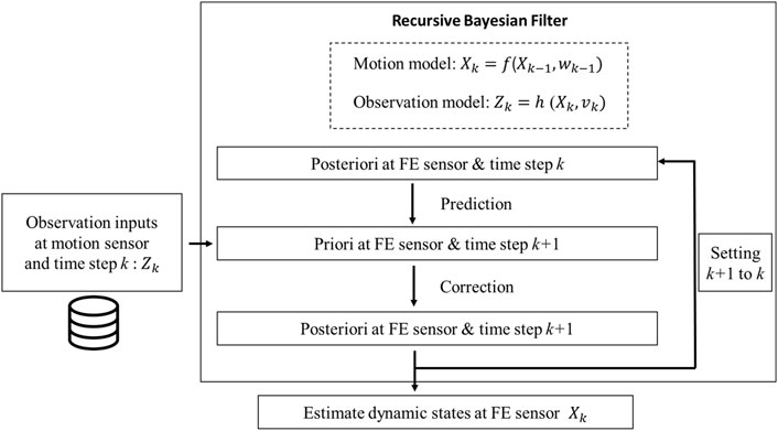
Figure 7. Recursive Bayesian filter workflow to estimate dynamic states at the formation evaluation sensor.
The instrumented roll tests that are believed to be the closest to the real drilling exercises are employed. The typical roll test system instrumented with the accelerometer is shown in Figure 8A. The impact ring is mounted onto the ground. The tool assembly under test goes through the center of the impact ring, and both ends of the tool are constrained with blocks and bearings that support the assembly in a horizontal configuration. The tool assembly under test can be different sizes ranging from 4.75″ to 8.25″ in the outer diameter, and the corresponding impact ring needs to be adjusted to accommodate the size of the tool assembly. A drive motor is used to rotate the tool assembly. The roller bearings that are located at each end of the tool assembly can prevent lateral deflection but allow for free rotation. Each bearing is paired with an end shaft, and the end shaft serves as an adapter that can be used for testing different tool assemblies. The drive shaft is equipped with a locking component that can secure the bearing to the shaft and prevent axial motion, while the tail shaft exhibits a rolled surface to allow for axial motion of the assembly. A drive belt connects the drive motor to the tool assembly, and the belt is flexible to allow for translation and rotation as the assembly rotates. A motor drives the assembly to the target operational speed commonly between 0 and 250 RPM. The bearings and drive motor are mounted to a steel frame securely cemented in the foundation such that the distance between the bearings may be adjusted to accommodate different assembly lengths. A high-speed camera with 250 frame per second (FPS) is placed near the impact with a tripod, which is used for recording the video of the lateral motion of the tool on the impact ring during the test. The acceleration can be, respectively, measured with the high frequency three-axis piezo-accelerometer (enDAQ Data Logger) mounted on the collar close to the impact ring. The sampling rates for the measurements of accelerations are 15 kHz. Then motion sensors are installed around the formation evaluation sensor as shown in Figure 8B, and integration of the acceleration collected from the motion sensor yields the velocity and further integration of the obtained velocity can produce the displacement, where appropriate filtering needs to be applied to remove the drift.
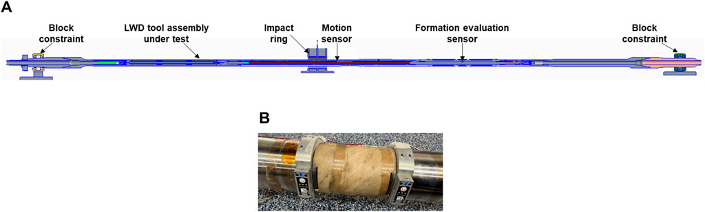
Figure 8. Full-scale roll test of LWD tool assembly: (A) laboratory setup (cross-sectional view), and (B) motion sensors mounted around the formation evaluation sensor.
A baseline BHA from a past field run in a 6.5-inch well with the LWD tool of interest located around the middle of the BHA is first considered, and well trajectory obtained from real survey is used in the simulation. Rotation speed of 80 RPM and surface weight on bit (WOB) of 21 klbf are simulated in the model. The drillstring simulations are first run and the results are compared to the field measurement sensor data for model calibration. The drillstring model is calibrated for the baseline job condition, and the calibrated drillstring model can be used to simulate many other scenarios to produce comprehensive synthetic dataset. The outputs from the drillstring beam model are then used as the inputs for the FEA solid model, and the transmissibility probability density functions in term of velocity and displacement can be generated accordingly (See Figure 6). The synthetic data at the motion sensor along with the transfer function can be used to predict the responses at the formation evaluation sensor location.
The lateral displacement of the centerline of the toolstring and orbital trajectories at the motion sensor and formation evaluation sensor are provided in Figure 9. Specifically, the red lines in Figure 9A denote the centerline of the toolstring, and the clearance between the toolstring and the wellbore can be outlined with the black lines; the results are given for both top view and side view at a representative time instant. One could see from the figure the variation of the OD along the toolstring that is considered in the simulation, and the clearance becomes smallest at the presence of stabilizers (Stabs); there is a large difference between the motion at the motion sensor and that at the formation evaluation sensor. A closer look at the accumulated orbital trajectories at the motion sensor and formation evaluation sensor in Figures 9B,C suggests much stronger motion magnitude at the formation evaluation sensor than at the motion sensor.
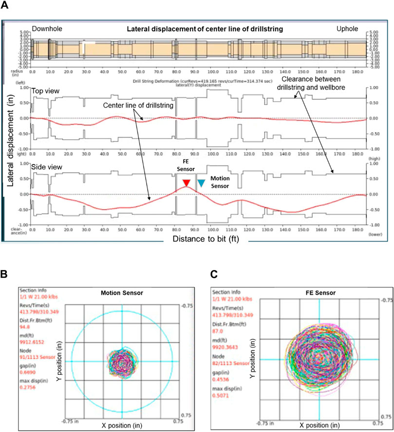
Figure 9. Simulation results obtained from drillstring beam model: (A) centerline displacement of drillstring at a representative time instant, (B) orbital trajectories at motion sensor, and (C) orbital trajectories at FE sensor. FE, Formation evaluation.
The comparison between transfer function prediction based on Eqs 4, 5, motion sensor measurements, and the true states at the formation evaluation sensor for the case with baseline BHA configuration can be found in Figure 10. In this case, the rotational speed is 80 RPM, and WOB is 21 klbf per the operational condition. Time windows with selected duration are sequentially applied to the original time-domain signals in a forward manner to compute maximum of the lateral displacement and mean of the lateral velocity as motion trajectory statistics, as shown in Figure 10A. The obtained map for lateral motion trajectories based on the statistics are shown in Figure 10B, where the red dots represent the trajectory at the motion sensor, the blue dots are the ground truth at the formation evaluation sensor, and the green dots are the responses predicted by the transfer function using the methodology described in Section 3.2. The statistics compute the mean of the lateral velocity and the maximum of the lateral displacement with the rolling time windows, and the duration of each time window is 2 s in this example. Apparently, one could see that the green dots are much closer to the blue dots than the red ones. In other words, if the motion sensor measurements were taken as the states of motions for the formation evaluation sensor, there would be more than a factor of 2 off in both velocity and displacement on the lateral motion trajectory map.
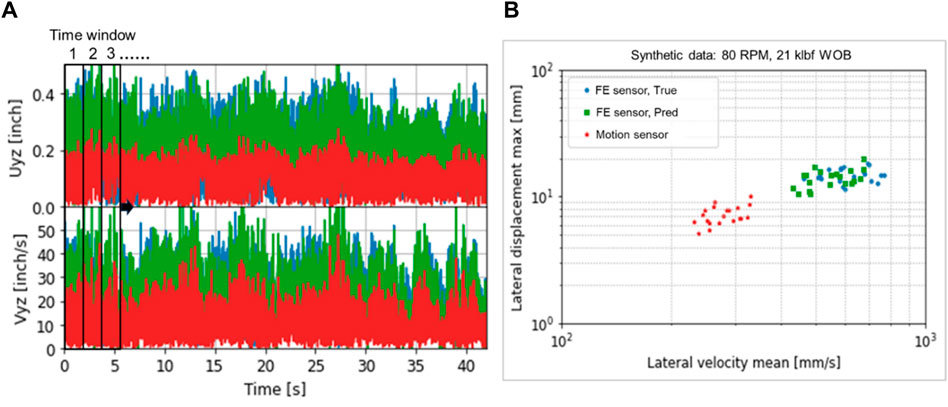
Figure 10. Comparison between transfer function prediction, motion sensor measurements, and the true states at the formation evaluation sensor for the baseline BHA configuration at 80 RPM and 21 klbf WOB: (A) signals in time domain, and (B) lateral motion trajectory map. FE, Formation evaluation.
Figure 10 shows only the results for the baseline BHA configuration and drilling condition. The model is also evaluated with additional cases for different drilling conditions in terms of combinations of RPM, WOB and well sizes. Table 1 summarizes the mean relative errors for velocity and displacement, respectively. In each of the parenthesis in the table, the first number corresponds to the velocity and the second number corresponds to the displacement. One can see that the maximum error is about 21% among different errors that are computed. Comparing this with the more than factor of 2 difference between the ground truth and motion sensor, it can be found that using transfer function can help significantly enhance the accuracy for the state estimations at the formation evaluation sensor location.
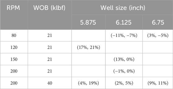
Table 1. Summary of mean relative errors for velocity and displacement, respectively. Mean Relative Errors (Velocity, Displacement).
Besides the baseline BHA with different drilling conditions in terms of RPM, WOB and well sizes (see Table 1), the robustness of the transfer function has been assessed with quite a few cases incorporating various BHA configurations used in field operation. The synthetic data for these cases are obtained by executing drilling dynamics simulations described in Section 3 offline, and these cases are defined with DOE (Design of Experiments) method (Barad, 2014). The parameters and their range used in the construction of the DOE matrix are based on operational need and summarized in Table 2. There are two stabilizers (Stabs) on the LWD tool of interest, and some stabilizers on other tools along the BHA, as shown in Figure 11. The size of the stabilizers, the distances between the stabs, and bit size are considered as BHA-related parameters. Furthermore, different well trajectories, and drilling conditions in terms of RPM and WOB are considered. Obviously for each parameter, a range of changes needs to be specified. There could be numerous combinations of these parameters. A random sampling technique called Latin hypercube sampling (Shields and Zhang, 2016) is used to effectively generate simulation matrix that contains a total of 60 cases.
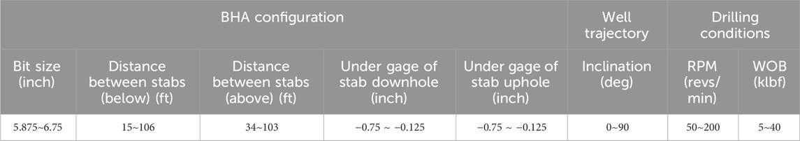
Table 2. Summary of parameters and their range for varying BHA configurations studied.
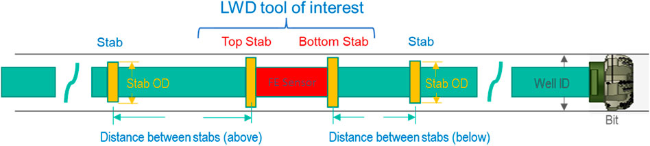
Figure 11. Schematic of varying BHA configurations. FE, Formation evaluation.
The DOE results obtained from drill dynamics simulations can then be used as the synthetic dataset to further evaluate the transfer function developed for the BHA. Whirling of the LWD tool occurred in 37 cases among the total of 60 cases that were simulated, in which 25 cases contain whirl only, and 12 cases involve transition between whirl and stable drilling. The remaining 23 cases are associated with stable drilling only. Figure 12 shows the overview of the obtained results for some representative cases in the DOE matrix for whirl only, stable drilling only, and whirl/stable drilling transition, respectively, with and without applying the transfer function. The motion sensor measurements, the prediction by the transfer function at the formation evaluation sensor according to Eqs 4, 5, and true states of motions at the formation evaluation sensor are overlaid in the figure for comparison. The motion trajectory statistics of maximum lateral displacement and mean lateral velocity are plotted in blue, light green, and brown, which represent the ground truth at the formation evaluation sensor, the transfer function prediction at the formation evaluation sensor based on Eqs 4, 5, and the measurements at the motion sensor, respectively. The statistics calculate the mean of the lateral velocity and the maximum of the lateral displacement with the rolling time windows, and the duration of each time window is 2 s (Also refer to Figure 10 for more details). As shown in the figure, with whirling only, the true motion trajectory at the formation evaluation sensor tends to carry higher risk for LWD quality due to its higher motion magnitude; under pure stable drilling, the trajectory at the formation evaluation sensor likely carries lower risk due to its smaller motion magnitude; interestingly, when there is a transition between whirl and stable drilling, the true motion trajectory at the formation evaluation sensor can be characterized by a long tail that crosses different risk zones. A closer look at the figure shows that there is obvious discrepancy between the ground truth at the formation evaluation sensor and the measurements at the motion sensor; however, applying the transfer function brings the estimation of the motion trajectory at the formation evaluation sensor much closer to the ground truth especially when whirling develops. To quantitively measure the prediction accuracy of the dynamic states, the mean and standard deviation (std) of the motion trajectories for the prediction by the transfer function and ground truth are provided with tabular values in the figure, where the first and second values in the parentheses denote lateral velocity mean, and lateral displacement max, respectively. These tabular values are calculated for every case defined in the DOE matrix, which are used to form the summary of relative errors to be elaborated in the following figure.
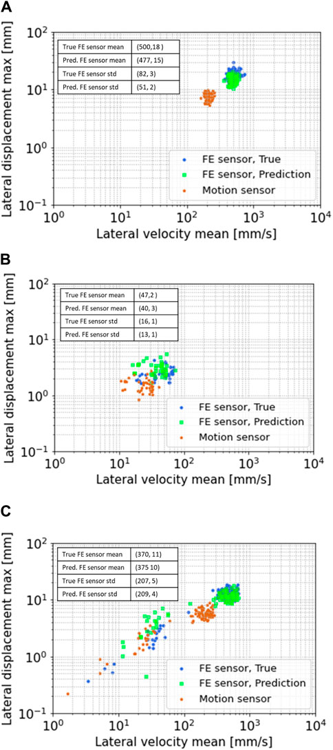
Figure 12. Lateral motion trajectories for representative cases in the DOE study based on synthetic data: (A) whirling only, (B) stable drilling only, and (C) whirl/stable drilling transition. FE, Formation evaluation.
After applying the same method and testing the transfer function to each case defined in the DOE matrix, the resulting distributions of mean and standard deviation (STD) relative errors of velocity and displacement for the cases of varying BHA configurations can be found in Figure 13, where the green and red dots represent the results for velocity and displacement with and without applying the transfer function, respectively. It can be learnt from Figure 13A that the mean relative error between the transfer function prediction based on Eqs 4, 5 and ground truth at the formation evaluation sensor is within 40% with a mean value of about 20% considering 99.3% confidence (the remaining 0.7% is by convention considered as outliers statistically). Without using the transfer function, the mean relative error between the motion sensor measurements and ground truth at the formation evaluation sensor can even get to 75% with the mean value of almost 60%. Similar observations can be found for the standard deviation (STD) relative error of the motion trajectories as well, as shown in Figure 13B. The comparative results indicate that overall, use of the transfer function can help reduce mean relative errors of velocity and displacement by almost a factor of 3 considering different BHA configurations and drilling conditions. It can be found that the vast majority of the cases are within the requirements for drilling operations, which significantly enhanced the confidence of proceeding with physical V&V with roll test data.
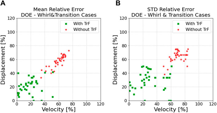
Figure 13. Summary of errors for the DOE study: (A) mean relative error, and (B) STD relative error.
In addition to the synthetic data obtained from drilling dynamics simulations in Section 5.1, physical test data described in Section 4 are also considered for further evaluating the developed modeling methodology. During experiments, backward whirl is triggered, and the accuracy of the developed transfer function is evaluated, which is elaborated as follows.
Figure 14 shows the experimental lateral motions of the LWD tool assembly when the rotation speed reaches 110 RPM. It can be observed that the friction between the LWD tool assembly and the impact ring causes the tool assembly to slide along the impact ring in the opposite direction of the rotation, in which backward whirl is excited, as shown in the figure. Figure 15 shows the comparison of lateral motion trajectories based on roll test data of backward whirl. In the figure, blue, light green, and brown represent the ground truth at the formation evaluation sensor, the transfer function prediction at the formation evaluation sensor according to Eqs 4, 5, and the measurements at the motion sensor, respectively. The prediction at the formation evaluation sensor matches reasonably well with the ground truth as shown in Figure 15, whereas large discrepancy is observed between the motion sensor data and the ground truth at the formation evaluation sensor. Similarly, the mean and standard deviation (std) of the motion trajectory clusters for the transfer function prediction and ground truth are given with tabular values in the figure to quantitively gauge the prediction accuracy of the motion states, in which the first and second values in the parentheses represent lateral velocity mean, and lateral displacement max, respectively. The relative errors between the prediction mean and ground true mean are 16.7% and 15.4% for lateral velocity mean and lateral displacement max, respectively, which are considered small for engineering applications. This once again demonstrates good confidence in utilizing this transfer function method to predict the responses from one point to another point.
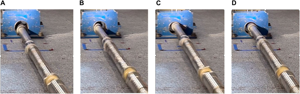
Figure 14. Motions of the LWD tool assembly at representative positions during backward whirl: (A) lowermost, (B) leftmost, (C) uppermost, and (D) rightmost.
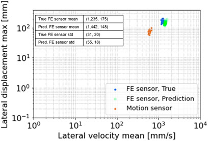
Figure 15. Comparison of lateral motion trajectories based on roll test data of backward whirl.
In this paper, a Bayesian data assimilation approach that can merge physics with motion sensor measurement is presented to estimate the dynamic states at points of interest on the BHA with proper uncertainty quantification. A 4.75 inch-LWD tool has been taken as the use case, in which the dynamic states at the formation evaluation sensor can be predicted in real time with the developed transfer function and the measurements at the motion sensor as the required inputs. The accuracy and precision of the transfer function has been assessed with synthetic data obtained from multi-fidelity drilling dynamics simulations for various BHA configurations and drilling conditions. It has been observed that the prediction by the transfer function matches favorably well with the true states of motion at the formation evaluation sensor. The developed transfer function method is further evaluated with experimental roll test data, which is considered as close to drilling conditions. It has been shown that the prediction by the transfer function is consistently close to the ground truth when whirling develops, which validates the developed data assimilation approach for drilling and measurement applications. Kalman Filter types assume that our belief in the states of the system can be approximately expressed with Gaussian. To achieve more accurate prediction, Particle Filter (PF) may be pursued in the future, which is more elastic as it is based on a sequential Monte Carlo method and does not assume Gaussian nature of noise in the data, but PF is more computationally expensive. However, the UKF approach selected in this study aims to provide a trade-off between the low computational effort of the Kalman filter and the high performance of the particle filter.
The raw data supporting the conclusions of this article will be made available by the authors, without undue reservation.
FS: Conceptualization, Data curation, Formal Analysis, Investigation, Methodology, Software, Visualization, Writing–original draft. KS: Conceptualization, Investigation, Methodology, Software, Writing–review and editing. KL: Conceptualization, Funding acquisition, Methodology, Project administration, Resources, Writing–review and editing. AM: Investigation, Resources, Writing–review and editing. SO: Conceptualization, Funding acquisition, Project administration, Resources, Writing–review and editing. IL: Conceptualization, Funding acquisition, Project administration, Resources, Writing–review and editing. RS: Resources, Validation, Writing–review and editing.
The author(s) declare financial support was received for the research, authorship, and/or publication of this article. This project is supported by SLB internal engineering funding.
The authors thank the SLB management for the permission to publish this work. Helpful inputs from Shin Utsuzawa, Albina Mutina, Faisal Esmail, Mike Langston, Haitao Zhang, Amandine Battentier, Yong Chang, Lu DeMortain, Liangyu Xu, Emilio de Matias Salces, Victor Barbe, Khaldon Hassan, Mike Ritchie, Mike Ritchie, Kang Zhang, Adam Bowler, Laurent Alteirac, Wei Chen, Yuelin Shen, Tianxiang Su, Muhannad Abuhaikal, Antoine Benard, Julien Converset, and Varun Sharma are thankfully acknowledged.
Authors FS, KS, KL, AM, SO, IL and RS were employed by SLB.
All claims expressed in this article are solely those of the authors and do not necessarily represent those of their affiliated organizations, or those of the publisher, the editors and the reviewers. Any product that may be evaluated in this article, or claim that may be made by its manufacturer, is not guaranteed or endorsed by the publisher.
Algu, D. R., Denham, W., Nelson, G., Tang, W., Compton, M. T., Courville, D. F., et al. (2008). “Maximizing hole enlargement while drilling (HEWD) performance with state-of-the-art BHA dynamic analysis program and operation road map,” in SPE annual technical Conference and exhibition (denver, Colorado, USA). SPE-115607-MS (USA: Society of Petroleum Engineers).
Argyris, J. H., Balmer, H., Doltsinis, J.St., Dunne, P. C., Haase, M., Kleiber, M., et al. (1979). Finite element method - the natural approach. Comput. Methods Appl. Mech. Eng. 17-18, 1–106. doi:10.1016/0045-7825(79)90083-5
Barad, M. (2014). Design of experiments (DOE) - a valuable multi-purpose methodology. Appl. Math. 5 (14), 48158. doi:10.4236/am.2014.514206
Chen, W., Shen, Y., Chen, R., Zhang, Z., and Rawlins, S. A. (2021). Simulating drillstring dynamics motion and post-buckling state with advanced transient dynamics model. SPE Drill Compl. 36 (03), 613–627. doi:10.2118/199557-pa
Chen, W., Shen, Y., Harmer, R., Rawlins, S., Dong, Y., and Chen, R. (2015). “Defining design and optimization method: dynamic simulation model produces integrated BHA solutions for efficient wellbore delivery,” in SPE/IADC drilling conference and exhibition (London, United Kingdom: Society of Petroleum Engineers). SPE/IADC-173008-MS.
Chen, W., Shen, Y., Zhang, Z., Bogath, C., and Harmer, R. (2019a). “Understand drilling system energy beyond MSE,” in SPE annual technical conference and exhibition (Calgary, Alberta, Canada: Society of Petroleum Engineers). SPE-196050-MS.
Chen, W., Yu, Y., Shen, Y., Zhang, Z., and Vesselinov, V. (2019b). “Automatic drilling dynamics interpretation using deep learning,” in SPE annual technical conference and exhibition (Calgary, Alberta, Canada: Society of Petroleum Engineers). SPE-195919-MS.
Coman, R., Thern, H., and Kischkat, T. (2018). “Lateral-motion correction of NMR logging-while-drilling data,” in SPWLA 59th annual logging symposium (London, UK: Society of Petrophysicists and Well Log Analysts). SPWLA-2018-LLL.
Gustafsson, F., and Hendeby, G. (2011). Some relations between extended and unscented Kalman filters. IEEE Trans. Signal Process. 60 (2), 545–555. doi:10.1109/tsp.2011.2172431
Haji, A., Tisdale, C., Muslem, M., Aramco, S., and Abouzaid, A. (2020). “Quantification and correction of lateral motion effects on NMR logging while drilling,” in Abu dhabi international petroleum exhibition and conference (Abu Dhabi, UAE: Society of Petroleum Engineers). SPE-203456-MS.
Hastermann, G., Reinhardt, M., Klein, R., and Reich, R. (2021). Balanced data assimilation for highly oscillatory mechanical systems. Commun. Appl. Math. Comput. Sci. 16, 119–154. doi:10.2140/camcos.2021.16.119
Hegdea, C., Millwaterb, H., and Graya, K. (2019). Classification of drilling stick slip severity using machine learning. J. Pet. Sci. Eng. 179, 1023–1036. doi:10.1016/j.petrol.2019.05.021
Hsu, T. W., Ou, S. H., Liau, J. M., Lin, J. G., Kao, C. C., Roland, A., et al. (2006). “Application of data assimilation for a spectral wave model on unstructured meshes,” in 25th international conference on offshore mechanics and arctic engineering (Hamburg, Germany: American Society of Mechanical Engineers). OMAE2006-92449.
Hursan, G., Silva, A., Van Steene, M., and Mutina, A. (2022). Learnings from a new slimhole LWD NMR technology. Petrophysics 63 (03), 389–403. doi:10.30632/pjv63n3-2022a7
Jansen, J. D. (1992). Whirl and chaotic motion of stabilized drill collars. SPE Drill. Eng. 7 (02), 107–114. doi:10.2118/20930-pa
Kapitaniak, M., Vaziri, V., Páez Chávez, J., and Wiercigroch, M. (2018). Experimental studies of forward and backward whirls of drill-string. Mech. Syst. Signal Process 100, 454–465. doi:10.1016/j.ymssp.2017.07.014
Kasumov, T., Valisevich, A., Zvyagin, V., Kozhakhmetov, M., Griffon, R., Mironov, A., et al. (2013). “Integrated BHA improves ROP by 62% in ERD operation saving 29 days rig-time, sets Russian lateral length record,” in SPE arctic and extreme environments technical conference and exhibition (Moscow, Russia: Society of Petroleum Engineers). SPE-166852-MS.
Li, C., and Xu, Z. (2023). A review of communication technologies in mud pulse telemetry systems. Electronics 12 (18), 3930. doi:10.3390/electronics12183930
Mohsan, M., Vossepoel, F. C., and Vardon, P. J. (2024). On the use of different data assimilation schemes in a fully coupled hydro-mechanical slope stability analysis. Georisk Assess. Manag. Risk Eng. Syst. Geohazards 18, 121–137. doi:10.1080/17499518.2023.2258607
Newmark, N. M. (1959). A method of computation for structural dynamics. J. Eng. Mech. Div. 85, 67–94. doi:10.1061/jmcea3.0000098
Pany, C. (2022). Investigation of circular, elliptical and obround shaped vessels by finite element method(FEM) analysis under internal pressure loading.
Pany, C. (2023). Large amplitude free vibrations analysis of prismatic and non-prismatic different tapered cantilever beams. Pamukkale Univ. Muh Bilim Derg. 29 (4), 370–376. doi:10.5505/pajes.2022.02489
Pany, C., and Rao, G. V. (2002). Calculation of non-linear fundamental frequency of a cantilever beam using non-linear stiffness. J. Sound. Vib. 256 (4), 787–790. doi:10.1006/jsvi.2001.4224
Pany, C., and Rao, G. V. (2004). Large amplitude free vibrations of a uniform spring-hinged beam. J. Sound. Vib. 271 (3-5), 1163–1169. doi:10.1016/s0022-460x(03)00572-8
Pany, C., Tripathy, U. K., and Misra, L. (2001). Application of artificial neural network and autoregressive model in stream flow forecasting. J. Indian Water Works Assoc. 33 (1), 61–68.
Rubio, P. B., Chamoin, L., and Louf, F. (2021). Real-time data assimilation and control on mechanical systems under uncertainties. Adv. Model. Simul. Eng. Sci. 8, 4. doi:10.1186/s40323-021-00188-3
Schweidtmann, A. M., Zhang, D., and von Stosc, M. (2024). A review and perspective on hybrid modeling methodologies. Digit. Chem. Eng. 10, 100136. doi:10.1016/j.dche.2023.100136
Shao, D., Chu, J., Chen, L., and Ma, H. (2023). Data assimilation with hybrid modeling. Chaos, Solit. Fractals 167, 113069. doi:10.1016/j.chaos.2022.113069
Shen, Y., Zheng, Z., Zhao, J., Chen, W., Hamzah, M., Harmer, R., et al. (2017). “The origin and mechanism of severe stick-slip,” in SPE annual technical conference and exhibition (San Antonio, Texas, USA: Society of Petroleum Engineers). SPE-187457-MS.
Shi, J., Dourthe, L., Li, D., Deng, L., Louback, L., Song, F., et al. (2022). Real-time reamer vibration predicting, monitoring, and decision-making using hybrid modeling and a process digital twin. SPE Drill Compl 38 (02), 201–219. doi:10.2118/208795-ms
Shields, M. D., and Zhang, J. (2016). The generalization of Latin hypercube sampling. Reliab. Eng. Syst. Saf. 148, 96–108. doi:10.1016/j.ress.2015.12.002
Simpson, D. A. (2017). Chapter two - well-bore construction (drilling and completions). Pract. Onshore Gas. Field Eng., 85–134. doi:10.1016/B978-0-12-813022-3.00002-X
Song, F., Li, K., and Xu, L. (2022). “FEA-based prediction and experimental validation of drilling tool lateral motion dynamics,” in ASME international mechanical engineering congress and exposition (Columbus, Ohio, USA: American Society of Mechanical Engineers). IMECE2022-96130.
Song, F., Xu, L., Zhang, H., and Li, K. (2023). “Analysis of roll dynamics with computer vision,” in ASME international mechanical engineering congress and exposition (New Orleans, LA, USA: American Society of Mechanical Engineers). IMECE2023-113164.
Tollefsen, E., Weber, A., Kramer, A., Sirkin, G., Hartman, D., and Grant, L. (2007). “Logging while drilling measurements: from correlation to evaluation,” in International oil conference and exhibition in Mexico (Veracruz, Mexico: Society of Petroleum Engineers). SPE-108534-MS.
Vamsi, A., Ansari, J., Mk, S., Pany, C., John, B., Samridh, A., et al. (2021). Structural design and testing of pouch cells. JES 5 (2), 80–91. doi:10.30521/jes.815160
Wang, B., Zou, X., and Zhu, J. (2000). Data assimilation and its applications. PNAS 97 (21), 11143–11144. doi:10.1073/pnas.97.21.11143
Wang, C., Li, X., Li, Y., Xu, W., and Liao, W. (2021). Analysis of the effect of whirl on drillstring fatigue. Nonlinear Dyn. Drill. Eng. (2021), 6666767. doi:10.1155/2021/6666767
Wikle, C. K., and Berliner, L. M. (2007). A Bayesian tutorial for data assimilation. Phys. D. Nonlinear Phenom. 230 (1-2), 1–16. doi:10.1016/j.physd.2006.09.017
Zhao, D., Hovda, S., and Sangesland, S. (2017). Whirl simulation of drill collar and estimation of cumulative fatigue damage on drill-collar connection. SPE Drill Compl. 23 (02), 286–300. doi:10.2118/187964-pa
Keywords: Bayesian data assimilation, real-time inference, hybrid modeling, data-model fusion, recursive Bayesian inference, unscented Kalman filter, drilling dynamics modeling, experimental roll test
Citation: Song F, Shi K, Li K, Mahjoub A, Ossia S, Loretz I and Serafim R (2024) A physics-informed Bayesian data assimilation approach for real-time drilling tool lateral motion prediction. Front. Mech. Eng 10:1410360. doi: 10.3389/fmech.2024.1410360
Received: 01 April 2024; Accepted: 22 May 2024;
Published: 12 June 2024.
Edited by:
Yijie Jiang, University of Oklahoma, United StatesReviewed by:
Shangyuan Jiang, University of Oklahoma, United StatesCopyright © 2024 Song, Shi, Li, Mahjoub, Ossia, Loretz and Serafim. This is an open-access article distributed under the terms of the Creative Commons Attribution License (CC BY). The use, distribution or reproduction in other forums is permitted, provided the original author(s) and the copyright owner(s) are credited and that the original publication in this journal is cited, in accordance with accepted academic practice. No use, distribution or reproduction is permitted which does not comply with these terms.
*Correspondence: Ke Li, S0xpMkBzbGIuY29t
Disclaimer: All claims expressed in this article are solely those of the authors and do not necessarily represent those of their affiliated organizations, or those of the publisher, the editors and the reviewers. Any product that may be evaluated in this article or claim that may be made by its manufacturer is not guaranteed or endorsed by the publisher.
Research integrity at Frontiers
Learn more about the work of our research integrity team to safeguard the quality of each article we publish.