An assessment of the effect of surface topography on coefficient of friction for lubricated non-conformal contacts

Determining an accurate state of lubrication is of utmost importance for the precise functionality of machine elements and to achieve elongated life and durability. In this work, a homogenized mixed-lubrication model is developed to study the effect of surface topographies on the coefficient of friction. Various measured real surface topographies are integrated in the model using the roughness homogenization method. The shear-thinning behavior of the lubricant is incorporated by employing the Eyring constitutive relation. Several Stribeck curves are generated to analyze the effect of roughness lays and root mean square (RMS) roughness on the coefficient of friction. The homogenized mixed lubrication model is validated against experimental rolling/sliding ball-on-disc results, and a good agreement between simulated and experimental coefficient of friction is found.

1 Introduction

Energy losses due to friction and wear make up to one-third of the total energy losses in engineering applications (Spikes and Olver, 2003; Prajapati and Tiwari, 2019a; Holmberg and Erdemir, 2019). The cost associated with the energy losses due to friction and wear is often very high (Holmberg et al., 2017; Danola and Garg, 2020). The primary aim of tribological analysis is often to reduce friction and wear between moving surfaces by promoting a lubricating film (Larsson, 1997). Most machines constitute of moving tribological components like, e.g., rolling element bearings, gears, and cams, and these operate under lubricated conditions in order to minimize losses due to friction and wear (Higashitani et al., 2023). Such non-conforming tribological components are expected to operate in the elastohydrodynamic lubrication (EHL) regime, which is in contrast to conformal contacts that operate in the hydrodynamic lubrication (HL) regime (Prajapati and Tiwari, 2019b). In the EHL regime, the applied pressure, which typically is in the GPa range, causes the lubricant viscosity to increase several orders of magnitude. In turn, this enables surfaces to yield elastically, and thus facilitates the formation a thin, sometimes only a few nanometer EHL film (Spikes and Zhnag, 2014). In addition, it is well established that all surfaces consist some level of surface-irregularities, even if produced using, e.g., super-finishing methods (Pawlus et al., 2020). As a result, and specially combined with the use of low viscosity lubricants (to reduce viscous losses) the film thickness in such contacts is sometimes too low to prevent asperity interactions, thus leading to mixed-lubrication (ML), or even worse, boundary lubrication (BL) (Spikes and Olver, 2003). In the BL/ML regimes, some fraction of the total transmitted load is carried by the lubricant film and the remaining is carried by the asperities causing increased friction, and wear (Taylor et al., 2020; Tang et al., 2023). Due to the significant amount of load carried by asperities in the boundary/mixed regime, knowledge of the role of surface topography on tribological conditions is crucial. Previously, it has been observed that a small change in the surface topography during operation (running-in) can lead to a significant improvement in a tribological contacts film formation ability (Hansen et al., 2019; Hansen et al., 2020a; Hansen et al., 2020b). Also, the surface topography.

In the mid of 20th century, stochastic models (roughness defined by statistical parameters) were developed to account for the surface contacts in the analysis of the ML regime (Christensen, 1969; Johnson et al., 1972; Patir and Cheng, 1978; Zhu and Cheng, 1988). The average flow model developed by Patir and Cheng (Patir and Cheng, 1978) is one of the most used stochastic models in the tribology community due to its satisfactory accuracy, simplicity and easy implementation (Hou et al., 2023). Although offering great simplicity, stochastic models usually do not provide sufficient localized information (e.g., film thickness breakdown or micro-EHL effects) that may be important in case of ultrathin film lubrication (Zhu and Wang, 2013). On the other hand, deterministic models (roughness defined at each grid node) certainly have great advantage due to consideration of 3D digitized real surface topography, and has been successfully used to simulate the thin and ultra-thin film lubrication conditions (Xu and Sadeghi, 1996; Zhu and Ai, 1997; Hu and Zhu, 2000; Zhu and Dowson, 2003; Zhu et al., 2015; Chong et al., 2019). However, there are several challenges (computational cost, solution schemes, discretization of Couette term, density derivatives, numerical stability, etc.,) in employing deterministic models, which researchers are dealing with in different ways (Wang et al., 2020). Apart from the Patir and Cheng (Patir and Cheng, 1978) average flow model, the homogenization method (Bayada and Chambat, 1988) which also is a kind of averaging method, have received much attention due to its accurate averaging results and applicability for arbitrary oriented rough surfaces (Rom et al., 2021). Different forms of the homogenized Reynold’s equations were derived to study both the stationary and transient lubricated contact problems (Bayada and Faure, 1989; Bayada et al., 2005; Almqvist and Dasht, 2006; Almqvist et al., 2007; Almqvist et al., 2011; Almqvist et al., 2012; Fatu et al., 2012). Unlike the Patir and Cheng average flow model (Patir and Cheng, 1978), the method of homogenization is not commonly used in tribology (Rom et al., 2021). In the past, the homogenized Reynold’s equation was used to study surface roughness and texture effects in conformal contacts (Bayada et al., 2005; Sahlin et al., 2010; Rom et al., 2021). Recently, the method has been employed in non-conformal contacts to study micro-EHL, and for the predicting the coefficient of friction in the ML regime (Hugo et al., 2019; Hansen et al., 2020; Hansen et al., 2023). A well-known challenge with the homogenization method is the fact that real engineered rough surfaces typically are not truly periodic, hence the employment of periodic boundary conditions is challenging, and an alternative approach is needed (Almqvist and Dasht, 2006). Hansen et al. (Hansen et al., 2023) solved the transient local-scale problem by employing Dirichlet boundary condition (χ₁ = χ₂ = χ₃ = 0) at one point of the domain faces and followed periodic boundary conditions in all other points of the domain faces (Hansen et al., 2023). It can be outlined from the above literature that the homogenization method has not been employed to predict the coefficient of friction (CoF) for counterformal contacts including shear-thinning and cavitation effects (Hugo et al., 2019; Hansen et al., 2020; Hansen et al., 2023). The aim of the present work is to use the homogenization method to investigate the surface topography effect on coefficient of friction by developing a mixed lubrication model for counterformal contacts. A linear approximation (Ehret et al., 1998) is used to simulate shear thinning behavior of non-Newtonian fluids. The validity of the homogenized mixed-EHL model is checked by comparing the CoF obtained from present simulation with those of rolling/sliding ball-on-disc experiments (Hansen et al., 2021). The effect of surface roughness lays and roughness on coefficient of friction is discussed in detail.

2 Simulation methodology

2.1 Lubricants properties and rheological model

It is well established that tribological properties significantly depend on the lubricant types (i.e., mineral, ester, ionic liquids, etc.,) and characteristics (rheological properties) of the fluid (Bjorling et al., 2013). In this work, Squalane (SQL) is chosen as reference fluid for mixed-lubrication analysis. SQL is a well characterized (experimentally and with MD simulations) lubricant and has extensively been used as a reference fluid in the EHD lubrication research (Bair, 2006; Xu et al., 2023). To describe the density of the lubricant (ρ), the Tait equation of state is used. The relative density (ρ/ρ_R) is derived (see Eq. 1) by determining the relative volume (V/V_R) for a given pressure and temperature. An expression for determining relative volume is given in Eqs 2–3 (Bair, 2006).

$\rho ={\rho }_R.\frac{V_R}{V}(1)$

$\frac{V}{V_R}=\left(1+a_v\left(T-T_R\right)\right).\left(1-\frac{1}{1+K_0^{\prime }}.\mathit{ln}\left[1+\frac{p_h}{K_0}.\left(1+K_0^{\prime }\right)\right]\right)(2)$

$K_0=K_{00}.\mathit{exp}\left(-{\beta }_{K}T\right)(3)$

where, K₀, $K_0^{\prime }$, a_v, β_K, T_R, are the parameters for Tait equation of state and can be obtained from Table 1 for SQL.

TABLE 1

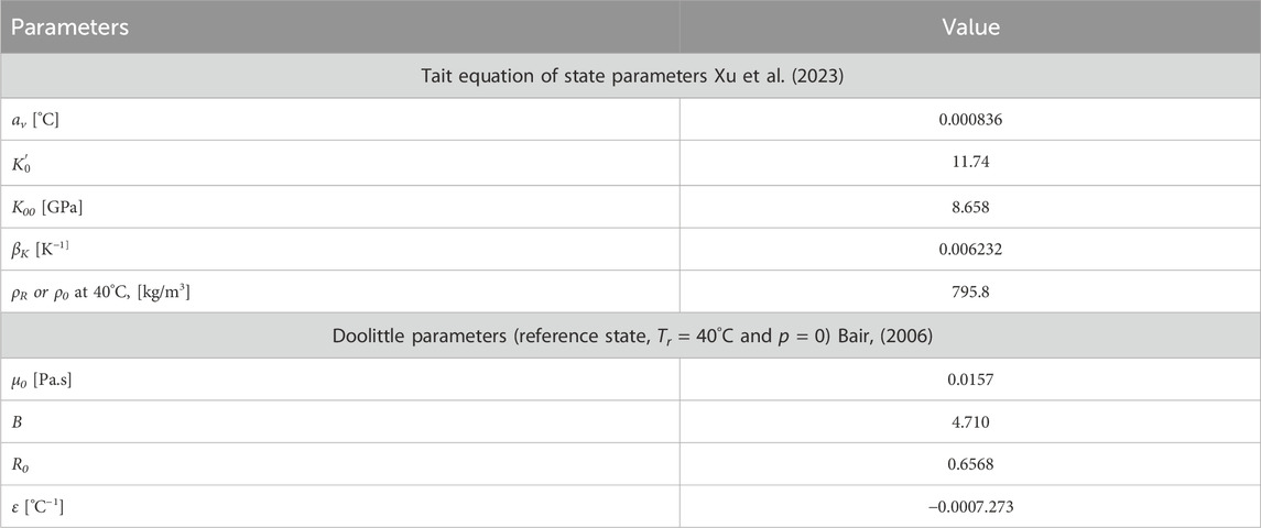
TABLE 1. Rheological parameters for Squalane (SQL).

Another important property is the viscosity of the lubricant which is significantly affected by the change in pressure and temperature. In this work, the Doolittle equation (see Eqs 4, 5) is used for determining the low shear viscosity or Newtonian viscosity (μ_N) (Bair, 2006). For the reference state (p = 0, T_r = 40 [°C]), the parameters involved in Eqs 4, 5 are given in Table 1. The variation of relative density (ρ/ρ_R) and Newtonian viscosity (μ_N) with pressure and temperature is presented in Figure 1.

${\mu }_N={\mu }_0\mathit{exp}\left[B{R}_0\left(\frac{\frac{V_{\infty }}{V_{\infty R}}}{\frac{V}{V_R}-R_0\frac{V_{\infty }}{V_{\infty R}}}-\frac{1}{1-R_0}\right)\right](4)$

$\frac{V_{\infty }}{V_{\infty R}}=1+\epsilon \left(T-T_R\right)(5)$

FIGURE 1

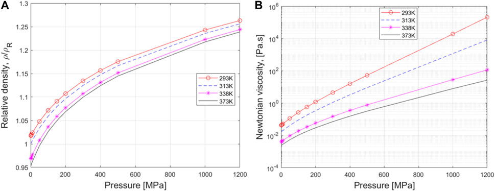
FIGURE 1. (A) Variation of relative density with pressure and temperature for squalane (B) variation of Newtonian viscosity with pressure and temperature for sqaualane.

In the literature, two rheological models, Eyring, (1936) and Bair, (2004) have extensively been used for the prediction of tribological properties. However, it is still debated which rheological model is more suitable for the prediction of traction coefficient (Bair, 2006). The Carreau–Yasuda–Bair shear-thinning equation relates generalized viscosity with shear stress involving four unknowns (Bair, 2004; Bair, 2006). Whereas, the Eyring shear-thinning equation (see Eqs 6, 7) involves only two parameters (Eyring stress and viscosity at ambient pressure), a simplicity that greatly facilitates the characterization process (Bair, 2006). Following the works of Jadhao and Robbins, (2019), a numerically fit expression of Eyring stress(τ_e) based on NEMD simulations was developed by Xu et al. (2023). Eq. 8 shows an expression of Eyring stress as a function of pressure (p) and temperature (T). The constants (a, b, c) used in the Eq. 8 can be found in Ref. Xu et al. (2023). Figure 2 represents the variation of Eyring stress with pressure (p) and temperature (T). It can be seen from Figure 2 that the Eyring stress significantly depends on pressure and temperature. In the present work, the Eyring stress for a specified load and lubricant temperature is calculated using Eq. 8, and further utilized to simulate the shear-thinning behavior of SQL. Readers are requested to see the recent works published by Xu et al. (2023) and Jadhao and Robbins (Jadhao and Robbins, 2019) to get an insight on the applicability of aforementioned rheological models that were based on NEMD simulation findings.

$\eta =\frac{{\tau }_e}{\dot{\gamma }}{\sinh }^{-1}\left(\frac{{\mu }_N\dot{\gamma }}{{\tau }_e}\right)(6)$

$\tau ={\tau }_e{\sinh }^{-1}\left(\frac{{\mu }_N\dot{\gamma }}{{\tau }_e}\right)(7)$

${\tau }_e\left(\text{MPa}\right)=a\left(T\right).\left(1-\mathit{exp}\left(-\frac{p}{b\left(T\right)}\right)\right)+c\left(T\right)(8)$

FIGURE 2

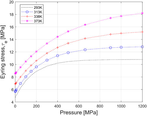
FIGURE 2. Variation of Eyring stress with pressure and temperature for squalane.

2.2 Brief description of global and local scales

Figure 3 represents a schematic of the global and local scale domains. The global-scale domain is the one over which EHL calculations are performed considering flow factors, and average quantities (average pressure and average film thickness distribution) are determined. The local-scale domain usually consists of a very small area ($A_l=L_{\xi 1}$. $L_{\xi 2}$), in comparison to the global-scale domain (L_x1. L_x2) as shown in Figure 3. As discussed in Refs. (Almqvist and Dasht, 2006; Almqvist et al., 2007; Almqvist et al., 2011; Almqvist et al., 2012), the local-scale length ($L_{\xi }$) in general should in general be less than 1/10 of the Hertzian contact radius (a_c) to get satisfactory accuracy in the flow factors. Following the scale-separation method introduced by Sahlin et al. (Sahlin et al., 2010), the global-scale gap height (h) between contacting bodies (upper and lower) can be fragmented into mean gap height (h_m) and deformed gap height (h_r) as shown in Eq. 9. It should be noted that in Eq. 9, the mean gap height depends only on the global-scale coordinates (x₁ and x₂), whereas, the deformed gap height depends on the global and local scale coordinates (x₁, x₂, ξ₁ and ξ₂) and time period (τ_r). The global-scale gap height is thus expressed as:

$h=h\left(x_1,x_2,\overrightarrow{\xi }\right)=h_m\left(h_0\left(x_1,x_2\right)\right)+h_r\left(h_0\left(x_1,x_2,\overrightarrow{\xi },{\tau }_r\right)\right)(9)$

where, x₁-and x₂-are the axis along and perpendicular to the rolling direction respectively, ξ₁ and ξ₂ are the axis along and perpendicular to the direction of movement of roughness respectively, and h₀ is the rigid body displacement at the local-scale.

FIGURE 3

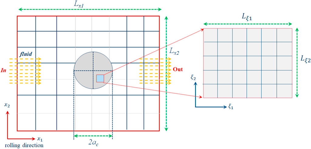
FIGURE 3. Schematic representation of global and -local scales.

2.3 Surface topography measurement

In this section, surface measurement process and pre-processing of roughness data is discussed. A Zygo New View 3D WLI profilometer (Zygo Corporation, United States) was used for an acquisition of surface roughness profiles using ×10 objective with ×0.5 field of view. All measured surface topography data was pre-processed (form removal using second degree polynomial, retrieval of roughness profile by applying 0.5 mm robust Gaussian filter) using MountainsMap Premium 10.0 (Digital Surf, France). From a larger measured area of each surface, a surface area of 558.9 × 558.9 was trimmed which consists of 256 × 256 sampling points. Isometric view of upper (S1, S2, S3, and S4) and lower body surface topographies are represented in Figures 4, 5. In this work, measured surfaces of balls are named as upper body surfaces and measured surface of a disc is named as lower body surface. Table 2 presents the calculated surface topography parameters for both upper and lower body surfaces. It can be observed from Figure 5 that the lower body has a mirror like surface finish (S_q = 0.003 [μm] from Table 2). The upper body surface roughness (S_q) is 0.047 [μm] for S1 and 0.112 μm for S2 - S4. The surface roughness of S2-S4 is rescaled from Ref. (Hansen et al., 2021) in order to facilitate the numerical comparison, while surface S1 is used without rescaling. The upper body surfaces (S2-S4) are specially prepared having different surface roughness lay (isotropic, S2; cross-hatched, S3; transverse, S4) with the same level of surface roughness (S_q). The upper body surface S1 has an isotropic roughness lay with comparatively lower roughness (S_q) than S2 to examine the role of surface roughness with fixed roughness lay.

FIGURE 4

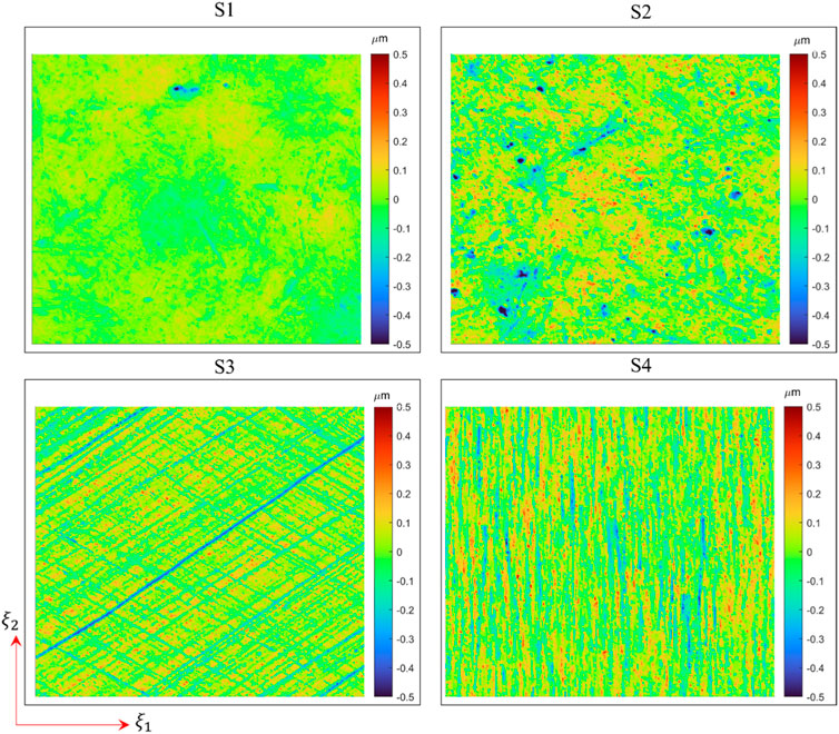
FIGURE 4. Isometric view of various surface topographies (S1-S4) of upper body.

FIGURE 5

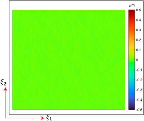
FIGURE 5. Isometric view of lower body surface topography.

TABLE 2

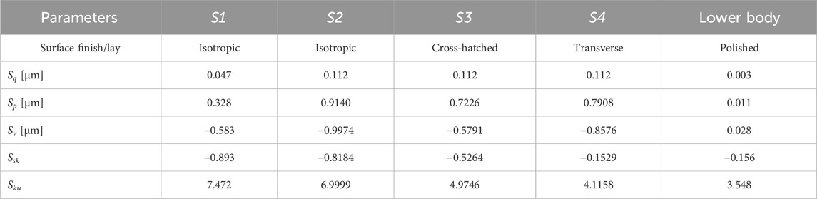
TABLE 2. Calculated surface topography parameters.

2.4 Local-scale analysis and calculation of flow factors

In this section, the local-scale treatment of the contacting bodies surface topography is discussed. From Section 2.3, it can be easily observed that the lower body surface is significantly smoother in comparison to the upper body surfaces. In the local-scale domain, flow factors, asperity pressure and mean gap are calculated by changing the rigid body displacement (h₀) from 2.5 [μm] −1 [nm] in 100 steps. For each rigid body displacement, 64 time steps are used to periodically move the upper body roughness over the lower body roughness. The averaging is performed over the local-scale domain lengths ($L_{\xi 1}$ and $L_{\xi 2}$) and periodic roughness time length (T_r). For a particular rigid body displacement (h₀), and at each time step (t), the asperity contact pressure (p_asp) and defomed gap height (h_l) distribution over the local domain (ξ₁ and ξ₂) is calculated. This is done by employing a boundary element method (BEM) based dry-contact solver, as previously reported by Akchurin et al. (2015). Outside the contact domain, the asperity contact pressure is set to zero, whereas, within the contact region, the asperity contact pressure varies between zero (lower limit) to the hardness of the material, H (upper limit). The input parameters used for the local-scale analysis are given in Table 3. After obtaining the deformed gap height (h_l), Eq. 10, Eq. 11, Eq. 12 are solved to determine the variables (χ₁, χ₂, χ₃) of the unsteady local-scale problem assuming incompressible and isoviscous fluid behavior. Eq. 10, Eq. 11, Eq. 12 are discretized using the finite volume method (FVM) (Hansen et al., 2023). A second order central interpolation scheme is used to discretize the spatial derivatives, whereas, a first order Euler implicit scheme is used to discretize the temporal derivative. Periodic boundary conditions are applied at all sides of the local-domain (Hansen et al., 2023). After solving all time steps, the average contact pressure (p_asp,avg), mean gap height (h_mean) and the average homogenization factors (A, $\overrightarrow{B}$, C and $\overrightarrow{D}$) can be determined using equations as given in Appendix A:

${\nabla }_{\overrightarrow{\xi }}.\left(h_l^3{.\nabla }_{\overrightarrow{\xi }}{\chi }_1\right)=\frac{\partial h_l}{\partial {\xi }_1}+\frac{1}{u_m}\frac{\partial h_l}{\partial t}(10)$

${\nabla }_{\overrightarrow{\xi }}.\left(h_l^3{.\nabla }_{\overrightarrow{\xi }}{\chi }_2\right)=-\frac{\partial h_l^3}{\partial {\xi }_1}(11)$

${\nabla }_{\overrightarrow{\xi }}.\left(h_l^3{.\nabla }_{\overrightarrow{\xi }}{\chi }_3\right)=-\frac{\partial h_l^3}{\partial {\xi }_2}(12)$

TABLE 3

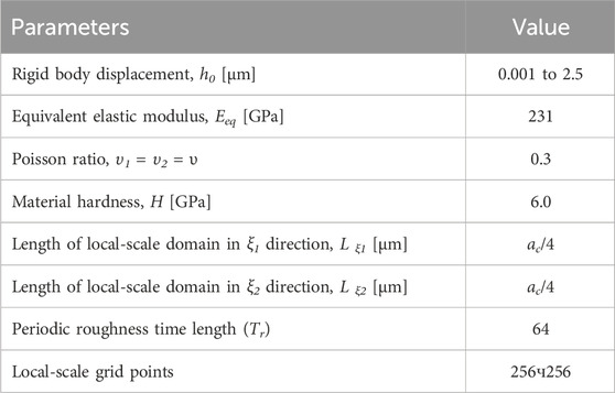
TABLE 3. Input parameters for the local-scale analysis.

2.5 Homogenized Eyring-Reynold’s equation

After solving the problem in the local-scale, the global-scale simulation is performed to get the average film thickness and average hydrodynamic pressure distribution. For the Eyring fluids, an expression of the homogenized Reynold’s equation with cavitation constraints is given in Eq. 13.

$\nabla .\left(\frac{{\rho }_l{h}_m^3}{12{\eta }_{eff}}.A.\nabla p_h-{\rho }_l{.h_m.u}_m.\overrightarrow{B.}\left(1-\theta \right)\right)=0(13)$

Cavitation constraints, $\theta .p_h=0,p_h\ge 0,\theta \ge 0$where, $u_m=u_{low}+u_{up}/2$ is the mean rolling speed, u_low is the surface speed of the lower body (faster), u_up is the surface speed of the upper body (slower), x₁-and x₂-are the axis along and perpendicular to the direction of motion respectively, θ = 1-ρ_m/ρ_l is the cavity fraction, ρ_m is the density of the mixture, ρ_l is the density of lubricant, h_m is the macroscopic mean gap height, A = $\left[\begin{array}{cc}{A}_{11}& A_{12}\\ A_{21}& A_{22}\end{array}\right]$ is the pressure flow factor and $\overrightarrow{B}$ = $\left[\begin{array}{c}{B}_1\\ B_2\end{array}\right]$ is the shear flow factor.

The term η_eff in Eq. 13 is the effective viscosity which includes shear-thinning effect according to linear approximation of Ehret and Dowson (Ehret et al., 1998). The effective viscosity is defined as given in Eq. 14 (Ehret et al., 1998).

${\eta }_{eff}=\left\{\begin{array}{c}{\eta }_{x1},\text{in\hspace{0.17em}}{x}_1\text{\hspace{0.17em}direction}\\ {\eta }_{x2},\text{in\hspace{0.17em}}{x}_2\text{\hspace{0.17em}direction}\end{array}\right.(14)$

${\eta }_{x1}=\frac{{\mu }_N}{f\left(q\right)+q.f^{\prime }\left(q\right)}$, ${\eta }_{x2}=\frac{{\mu }_N}{f\left(q\right)}$, $f\left(q\right)=\frac{\mathit{sinh}\left(q\right)}{q}$where, $q=\left({\mu }_N{.u}_s/h_m.{\tau }_e\right)$, u_s (SRR.u_m) is the sliding speed, SRR (u_low-u_up/u_m) is the slide-to-roll ratio.

It can be realized that the homogenized flow factors, the average asperity pressure and mean gap (h_mean) are a function of microscopic (local scale) rigid body displacement (h₀). Their values are interpolated in the global-scale by considering that the macroscopic gap height in the global-scale is the same as the rigid body displacement (h₀) in the local-scale (Sahlin et al., 2010). During the interpolation, the macroscopic gap height is replaced with h_mean whenever it falls below min (h₀). An expression of macroscopic gap height (h₀) is given in Eq. 15.

$h_0\left(x_1,x_2\right)=h_d+\delta \left(x_1,x_2\right)+h_g\left(x_1,x_2\right)(15)$

where, h_d is the rigid body approach, h_g is the gap height due to geometry of contacting bodies, and $\delta$ is the elastic deformation of the contacting bodies in the global-scale. An assumption of elastic-half space allows to express an equation of elastic deformation as given in Eq. 16 (Hansen et al., 2023).

$\delta \left(x_1,x_2\right)=\frac{2}{\pi E_{eq}}.{\iint }_{A_H}\frac{p_h\left(x_1^{\prime },x_2^{\prime }\right)+p_{asp,avg}\left(x_1^{\prime },x_2^{\prime }\right)}{\sqrt{{\left(x_1^{\prime }-x_1\right)}^2+{\left(x_2^{\prime }-x_2\right)}^2}}.d{x}_1^{\prime }.d{x}_2^{\prime }(16)$

Eq. 16 can be expressed in terms of a Kernel function (K) by discretizing the global-scale domain (A_H) into rectangles using the boundary element method. An expression of the elastic deformation in dependency of the Kernel function is given in Eq. 17. The Fourier transform method is used to accelerate the evaluation of Eq. 17 (Hansen et al., 2020).

$\delta \left(x_1,x_2\right)={\displaystyle \sum _{x_1^{\prime }}}{\displaystyle \sum _{x_2^{\prime }}}K\left(x_1-x_1^{\prime },x_2-x_2^{\prime }\right).\left(p_h\left(x_1^{\prime },x_2^{\prime }\right)+p_{asp,avg}\left(x_1^{\prime },x_2^{\prime }\right)\right)(17)$

2.6 Calculation of coefficient of friction

The friction force due to the fluid film is calculated by integrating the fluid shear stress (${\tau }_h$) over the hydrodynamic area (A_H). The expression for calculating the fluid shear stress is given in Eq. 18 (Hansen et al., 2023). The shear stress (${\tau }_{cont}$) due to asperity contacts is calculated according to Eq. 19. Finally, the total friction force is determined using Eq. 20. The CoF is calculated (see Eq. 21) by dividing the total friction force (F_total) by the total applied load (F_N).

${\tau }_h=\pm \frac{h_m}{2}.C.\nabla {\mathrm{p}}_h+\frac{{\eta }_{eff}}{h_m}.\left(-6.u_m.\overrightarrow{D}+u_r.\left[\begin{array}{c}1\\ 0\end{array}\right]\right).\left(1-\theta \right)(18)$

${\tau }_{cont}=f_{bc}.\left(p_{asp,avg}\right)(19)$

${\tau }_{total}={{\tau }_h+\tau }_{cont}$

$F_{total}=\iint {\tau }_{cont}.d{x}_1.d{x}_2+\iint {\tau }_h.d{x}_1.d{x}_2(20)$

$CoF=\frac{F_{total}}{F_N}(21)$

where C = $\left[\begin{array}{cc}{C}_{11}& C_{12}\\ C_{21}& C_{22}\end{array}\right]$ and $\overrightarrow{D}$ = $\left[\begin{array}{c}{D}_1\\ D_2\end{array}\right]$ are the shear stress flow factors, f_bc is the boundary friction coefficient which has been found in the range of 0.1–0.199 based on experimental results for hydrocarbon-based lubricants (Taylor and Sherrington, 2022). In this work, the boundary friction coefficient is set to 0.12.

2.7 Solution method for homogenized Eyring-Reynold’s equation

To get the average hydrodynamic pressure and average film thickness distribution, Eqs. 13, 15 and 16 are needed to discretize over the EHL domain (A_H). Similar to the FEM (finite element method) and FDM (finite difference method), the FVM (finite volume method) has extensively been used to solve the problems involving solid-fluid interactions (Ferziger et al., 2020). In this work, the homogenized Eyring-Reynold’s equation (Eq. 13) is discretized employing FVM. The Poiseuille terms are discretized using second order central interpolation scheme (Ferziger et al., 2020). The Couette term is discretized using first order upwind interpolation scheme (Ferziger et al., 2020). The FBNS (Fischer–Burmeister–Newton–Schur) solver has previously been used by Prajapati et al. (2022) to the study of piston/ring conjunction under mixed-lubrication condition. An extension (inclusion of elastic deformation in film thickness equation) of the FBNS solver for EHL non-conformal contacts has been recently reported in Ref. (Hansen et al., 2022). In this work, the EHL-FBNS solver is employed to solve the discretized form of EHL governing equations. The Dirichlet boundary conditions of p_h = 0 is employed at all sides (east, west, north, south) of the domain boundaries. Furthermore, the Dirichlet boundary condition of θ = 0 was used at the domain inlet (west), whereas the Neumann conditions were used for the cavity fraction at the remaining (east, north, south) boundaries. The PID controller is used to update the macroscopic rigid body displacement (h_d) (Wang et al., 2019). The iteration continues until the residual values (Hansen et al., 2022) becomes less than 10⁻⁶. For more information on the solution of the homogenized mixed lubrication equations, readers are referred to similar work recently published by Hansen et al. (Hansen et al., 2023). The operating conditions and other input parameters for the mixed-lubrication analysis are given in Table 4 and used throughout in this study unless otherwise specified.

TABLE 4

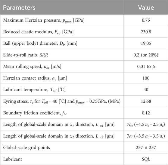
TABLE 4. Input parameters for mixed-lubrication analysis.

3 Results and discussion

Firstly, the accuracy of the homogenized mixed lubrication model is evaluated in terms of ranking by comparing the CoF obtained from present simulation and published results. Furthermore, the results obtained from local-scale analysis are discussed in detail. The influence of surface roughness lay (for same level of S_q) on the CoF is also discussed in detail, and finally, the influence of surface roughness on the CoF is investigated.

3.1 Validation of the homogenized mixed-lubrication model

To validate the homogenized mixed lubrication model, the ball (upper body) and disc (lower body) surface profiles previously reported by the authors (Hansen et al., 2021) are utilized. Hansen et al. (Hansen et al., 2021) calculated an improved film parameter (Λ^*) for pre (unworn) and post (after lift-off) surfaces having different roughness lay (transverse, longitudinal and isotropic), but the CoF’s were not reported there although measured. In this section, the CoF’s of the pre-test transverse and isotropic surfaces are disclosed and compared. The lower body (disc) surface had a mirror like surface finish in comparison to the ball surfaces (transverse, and isotropic) (Hansen et al., 2021). For the transverse and isotropic surfaces, the measured RMS roughness (S_q) was 0.287 [μm] (Hansen et al., 2021). The disc surface roughness (S_q) was limited to 3 nm (Hansen et al., 2021). The experiments were performed using a WAM (Wedeven Associates Machine) ball-on-disc test rig (Hansen et al., 2021). More detail on the working procedure of WAM ball-on-disc test rig can be found in Ref. [55, Section 2.2]. The exact surface roughness profiles data, experimental operating conditions, and lubricant (polyalphaolefins, PAO) properties as described in Ref. (Hansen et al., 2021) are adopted for validation of the model. The input parameters used in the simulation (for both local and global scale analysis), only for model validation are given as follows: p_max = 1.69 [GPa], E_eq = 231 [GPa], Hardness (H) = 6.9 [GPa], D_b = 20.64 [mm], a_c = 240 [μm], L_ξ = L_ξ1 = L_ξ2 = a_c/10, u_m = 1 [m/s], SRR = 1, f_bc = 0.12, S_q = 0.287 [μm], T_oil = 50 [°C], ρ₀ = 836 [kg/m³], μ₀ @ 50 [°C] = 57.48 [mPa.s], α @ [°C] = 14.317 [GPa^-1]. Roeland’s viscosity-pressure and DH (Dowson–Higginson) density-pressure relations are used to consider the piezoviscous and compressible effects (see Appendix B). Figure 6 represents the comparison between predicted and experimentally determined CoF’s for the transverse and isotropic rough surfaces. It can be observed that the rankings are the same, although the predicted CoF values are slightly less in comparison to the true value (experimental) for both surface roughness lays. A maximum absolute relative deviation ($\left|true-pred/true\right|\times 100$) of 15% is observed. This discrepancy likely originates from the fact that the rolling/sliding experiments in Ref. (Li et al., 2022) were performed for a relatively high Hertzian contact pressure, p_max = 1.69 [GPa], which is challenging from a modelling perspective since the oversimplified rheological relations (Roeland’s and DH relations) may not be the most accurate (Bair, 2004; Bair, 2006; Bjorling et al., 2013; Xu et al., 2023). Another source of error may be due to the assumed value of boundary friction coefficient (f_bc = 0.12). Nonetheless, overall, the results are reasonable and it can be concluded that the homogenized ML model presented in this work can be employed to predict the CoF for heavily loaded non-conformal contacts within acceptable accuracy.

FIGURE 6

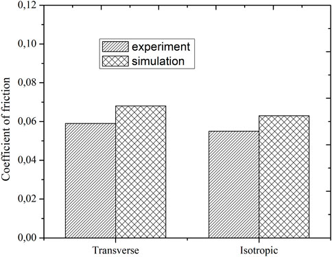
FIGURE 6. Experimental and numerical (simulation in present work) comparison of coefficient of friction for transverse and isotropic surfaces.

3.2 Flow factors, average asperity pressure and mean gap

Figures 7A–F shows the variation of pressure and shear flow factors as a function of microscopic rigid body displacement (h₀) for different rough surfaces. The flow factors (A₁₂ and A₂₁) are defined as cross-linked (coupled) pressure flow factors. Whereas, the main diagonal flow factors A₁₁, A₂₂ are defined as pressure flow factors and are calculated along and perpendicular to the rolling direction (x₁ direction) respectively. Similarly, the shear flow factors, B₁ and B₂ are calculated along and perpendicular to the rolling direction respectively. A change in the magnitude of the flow factors depend on several factors such as the asperity orientation (roughness lay), surface roughness (S_q) and rigid body displacement (h₀). The low value of the h₀ increases asperity-to-asperity contacts resulting in an increase in restriction in main flow, and as a result the change in the flow factors occur. At high value of the h₀ flow factors approaches 1 due to negligible asperity contacts. It can be seen from Figure 7A that the flow factor, A₁₁ variation with h₀ for isotropic surfaces is almost same, i.e., A₁₁ < 1 at the same h₀ for both S1 and S2. However, for h₀ < 0.25 [μm], a large reduction in A₁₁ is observed for S2 due to an increase the pressure flow resistance. At very low h₀, the higher surface roughness of S2 results in an increase in the main flow (pressure flow in x₁ direction) resistance. As illustrated in Figure 7A A₁₁ for the cross-hatched surface (S3) increases for h₀ <1[μm]. This happens due to the lower resistance to the pressure flow in the x₁ direction. For the transverse surface (S4), side flow increases which results in an increase in the resistance to the main flow (x₁ direction). As a result, a significant decrease in A₁₁ is observed for h₀ < 1 [μm]. As expected, at higher h₀ (>1 [μm]), A₁₁ approaches 1 for all types of rough surfaces which indicates a negligible effect of surface roughness. Figures 7B, C represent the variation of cross-linked pressure flow factors (A₁₂ and A₂₁) with an increase in h₀ from 1 [nm] - 2.5 [μm]. It can be observed that the variation in cross-linked pressure flow factors is almost negligible for S1, S2 and S2. However, significant variation in A₁₂ and A₂₁ is observed for the cross-hatched surface (S3). For h₀ <1 [μm], A₁₂ and A₂₁ asymptotically increase due to an increase in the main flow or a decrease in resistance to the main flow. Figure 7D represents the pressure flow factor (A₂₂) variation as a function of h₀ for various rough surfaces. For isotropic rough surfaces (S1 and S2), A₂₂ asymptotically increases with an increase in h₀. Whereas, cross-hatched and transverse rough surfaces exhibit an asymptotic decrease in A₂₂ with an increase in h₀.

FIGURE 7

FIGURE 7. (A–D) Pressure flow factors, A₁₁, A₁₂, A₂₁, A₂₂ (E, F) shear flow factors, B₁ and B₂ as a function of microscopic rigid body displacement (h₀) for different rough surfaces.

Figure 8A represents the asperity pressure curves (P_asp,avg vs h₀) for different rough surfaces. It can be seen that the average asperity pressure asymptotically increases with a decrease in rigid body displacement (h₀) for different rough surfaces (S1-S4). It can also be observed that for h₀ > 0.764 [μm] the average asperity pressure is zero for all rough surfaces due to the absence of asperity-to-asperity contacts. For isotropic rough surfaces, S1 and S2 the first non-zero value of average asperity pressure is found at h₀ = 0.347 [μm] and 0.895 [μm] respectively. Whereas, for the rough surfaces, S3 and S4 the first non-zero value of average asperity pressure occurs at h₀ = 0.764 [μm]. As illustrated in Figure 8A the average asperity pressure (P_asp,avg) for S1 is lower than the average asperity pressure for other rough surfaces (S2-S4). This happens due to a difference in the level of surface roughness between S1 and the other (S2-S4) rough surfaces. An expanded view of P_asp,avg (h₀) for S2-S4 is also presented as an inset in Figure 8A. It can be observed that for a particular value of h₀, the isotropic surface (S2) exhibits the lowest asperity pressure and the transverse surface (S4) exhibits the highest asperity pressure. The reason is a significant difference in the topographical properties, namely, the surface roughness lays. It should, however, be noted that parameters such as skewness and kurtosis are difficult to control in the surface preparation process and these may also have had a significance to asperity contact pressure.

FIGURE 8

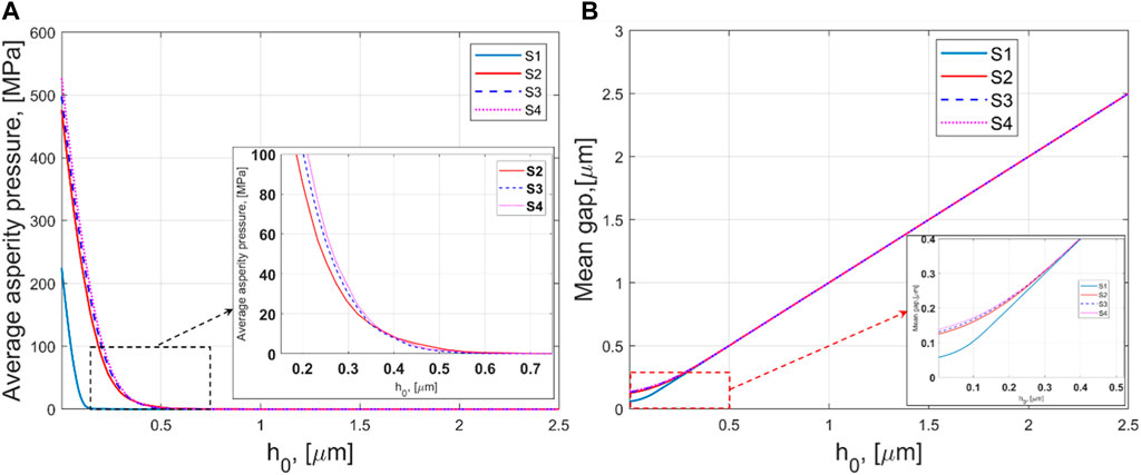
FIGURE 8. (A) Average asperity pressure, p_asp,avg (B) mean gap, h_mean as a function of microscopic rigid body displacement (h₀) for different rough surfaces.

Figure 8B represents the variation of mean gap (h_mean) as a function of h₀ for the different rough surfaces. The mean gap is defined as the distance between the smooth surface (lower body, stationary) mean plane and the mean plane of the deformed rough surface (upper body, moving). A linear variation between h_mean and h₀ is observed for a decrease in the rigid body displacement from 2.5 [μm] - 0.5[μm]. The value of h_mean equal to h₀ ideally indicates a no asperity-to-asperity contacts situation (h₀ < maximum peak height of a particular surface). However, a further decrease in h₀ results in a deviation between h_mean and h₀ for different types of rough surfaces (S1-S4) due to direct asperity-to-asperity contacts. In practical terms, when it comes to the pressure curves, it is desirable that the asperity pressure increases at lower rigid body displacement, h₀ (or mean gap in the global-scale), since P_asp,avg ≥ 0 can be ideally supposed to mark the onset of ML from the full film regime. For example, comparing S1 (isotropic, smooth) and any of the other rougher surfaces at, e.g., h₀ = 0.05 [μm], it can be realized that S1 will suffer significantly less surface distress, which is in line with well establish literature. In contrast, the influence of roughness lay is comparably much smaller, although, at least two notable differences can be observed under close inspection (inset plot). Firstly, it can be seen that the onset of ML occurs at thinner film for the S4 (transverse, h₀ = 0.764 [μm]) compared to the S2 (isotropic, h₀ = 0.895 [μm]), likely since the transversal surface yields better film forming ability than the isotropic, as demonstrated by the authors in Ref (Hansen et al., 2021). Secondly, and notably, due to the differences in surfaces stiffness, there is an intersection point (h₀ = 0.35 [μm]) that apparently makes the S2 (isotropic) more favorable (less asperity pressure/surface distress) than the S4 (transverse) in the ML- and towards the BL-regime. Clearly, both roughness height and lay is important when preparing surfaces for lubricated machine elements such as, e.g., rolling element bearings.

3.3 Influence of surface roughness on the coefficient of friction

Previously, it has been observed that surface roughness plays a dominant role in the mixed-lubrication regime (Zhu and Cheng, 1988; Hansen et al., 2019; Hansen et al., 2020a; Hansen et al., 2020b; Taylor et al., 2020; Tang et al., 2023). Here the present homogenized mixed-lubrication model is employed to see the influence of surface roughness on the CoF. As stated in Section 2.3, the rough surfaces S1 and S2 have similar roughness lay (isotropic) but there is a difference in their surface roughness height (S_q). The average flow factors, average asperity pressure and mean gap obtained from local-scale analysis are stored and further used in the global-scale to determine the CoF and asperity load ratio ($L_a=\left(F_{asp}/F_T\right)\times 100$) for various rolling speeds (u_m = 0.01 [m/s] - 6 [m/s]). For each rolling speed, the CoF and L_a are calculated and the corresponding data is presented in Figures 9A, B. As illustrated in Figures 9A, and as anticipated, the CoF decreases with an increase in rolling speed for both S1 and S2. Within the range of rolling speeds (u_m = 0.3 [m/s]—6 [m/s]), the relatively smooth surface (S1) exhibits lower CoF in comparison to the rough surface (S2). However, at very low rolling speed (u_m = 0.01 [m/s]) the CoF approaches the boundary friction coefficient value (f_bc = 0.12) for both surfaces. Another interesting observation is the EHL lift-off speed (u_m = 3 [m/s]) that is observed only for S1, whilst the S2 requires higher speeds. For rolling speed > 3 m/s a slight increase in the CoF is observed for S1 due to dominant viscous effects. However, for rough surface (S2) the CoF decreases gradually with an increase in rolling speed up to 6 [m/s]. Figure 9B represents the variation of asperity load ratio with an increase in rolling speed. It can be observed that the asperity load ratio decreases with an increase in rolling speed. For the rough surface S1, the asperity load ratio is almost negligible for rolling speed >1 [m/s]. Whereas, for the rough surface S2, some fraction of the total load is carried by asperities within the range of rolling speed (0.01[m/s] - 6 [m/s]). This happens due to the higher roughness of the S2 surface which causes more ML and thus increased asperity pressure or asperity load ratio.

FIGURE 9

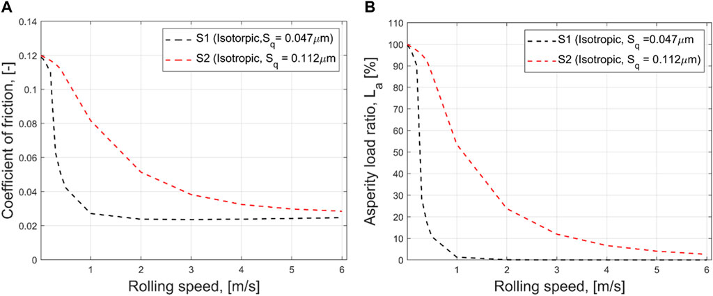
FIGURE 9. (A) Simulated Stribeck curves (B) Asperity load ratio curves for different level of surface roughness, (p_max = 0.75 [GPa], SRR = 20 [%], D_b = 19.05 [mm], f_bc = 0.12, τ_e = 12.68 [MPa], input surfaces = S1, S2, lubricant = SQL).

3.4 The influence of surface roughness lay on the coefficient of friction

In this section, the effect of surface roughness lay on the CoF and asperity load ratio (L_a) is discussed. The results (flow factors, average asperity pressure and mean gap) obtained from the local-scale analysis for rough surfaces, S2, S3, S4 are used in the global-scale to predict the CoF and asperity load ratio for a range of rolling speeds (0.01 [m/s]- 6 [m/s]). Figure 10A represents the variation of the CoF with an increase in rolling speed. It can be seen that the CoF decreases gradually with an increase in rolling speed for rough surfaces, S2-S4. As illustrated in Figure 10A at low rolling speeds (u_m < 0.5[m/s]), the CoF is nearly equal to boundary friction (f_bc = 0.12) for all rough surfaces, and the surface roughness lay is almost negligible due to severe asperity-to-asperity contacts. At slightly higher rolling speed, the surface roughness lay effects are clearly visible. For rolling speed (u_m = 0.5 [m/s]—4 [m/s]) the isotropic rough surface (S2) exhibits the lowest coefficient of friction, whereas, for cross-hatched (S3) and transverse (S4) rough surfaces, a slight difference in CoF values is found. At high rolling speeds, the CoF for the S2 and S3 is almost the same. The reason being that, as the contact exceeds the EHL lift-transition, the asperity load share becomes insignificant and viscous shear effect becomes dominant. However, for S4, a slightly higher CoF is observed at high rolling speeds. This happens due to the weak entraining action (or high lateral flow) for the transverse surface, which has the asperity orientation perpendicular to rolling direction. This weak entraining action leads to an increase in the shear stress flow factors, and hence cause an increase in the CoF. The similar variation in the CoF with an increase in rolling speed for different surface roughness lays has been reported in Ref. (Zhu and Wang, 2013).

FIGURE 10

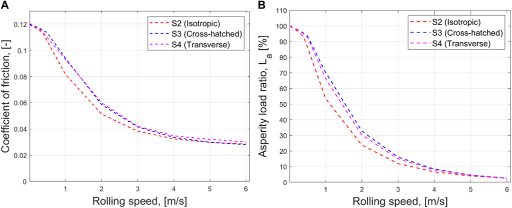
FIGURE 10. (A) Simulated Stribeck curves (B) Asperity load ratio for different rough surfaces, [p_max = 0.75 (GPa), SRR = 20 (%), D_b = 19.05 (mm), f_bc = 0.12, τ_e = 12.68 (MPa), input surfaces = S2, S3, S4, lubricant = SQL].

Figure 10B presents the variation of asperity load ratio with an increase in rolling speed for different surface roughness lays. As expected, the asperity load ratio gradually decreases with an increase in rolling speed. At low rolling speed, the asperity load ratio for all rough surfaces (S2-S4) approaches 100% indicating that most of the load is carried for by the asperities for S2, S3, S4. However, for rolling speeds 0.5 [m/s] and 3.5 [m/s], the asperity load values for different surface roughness lay are clearly distinct. The reason for getting the differences in the asperity load ratio is due to the different asperity orientation (roughness lay) for rough surfaces, S2-S4. The difference in the asperity orientation results in the significant change in magnitude of flow factors and asperity pressure. This change in the asperity pressure and flow factors leads to a variation in the asperity load ratio (L_a) value for rough surfaces, S2-S4. It can be inferred from Figure 10 that roughness lays potentially affect the CoF and L_a. As stated in the previous section, the CoF is determined assuming the steady state condition. It has also been observed that surface topography profoundly affects the wear process (Li et al., 2022). The studied roughness lays (isotropic, cross-hatched, and transverse) may affect also affect the wear process due to a change in the asperity pressure with an increase in number of cycles (Grützmacher et al., 2019). Understanding the evolution of surface topography over time will helps to improve the reliability and life of the tribological components (Grützmacher et al., 2019; Li et al., 2022).

4 Conclusion

This work deliberates the applicability of the homogenized mixed-lubrication model for heavily loaded non-conformal contacts. Various types of real engineering surface topographies (isotropic, cross-hatched, and transverse) acquired using an optical (non-contact) profilometer are used as input to the model. Simulations over a broad span of rolling speed are then conducted to investigate the effect of surface roughness height and lay (for the same S_q) on the asperity load ratio and the coefficient of friction (CoF). The main findings from the present work can be summarized as follows:

• A maximum relative absolute deviation of 15% is found when comparing the experimental and numerical CoF’s for transverse and isotropic surfaces. The assumption of boundary friction coefficient (f_bc) and possible oversimplified rheological relations may be the reasons for this discrepancy which may yet be considered reasonable for a rapid non-fully-deterministic model of this kind.

• The model captures the overall effects observed experimentally, including CoF ranking for various surface roughness height and lays within the range of rolling speed considered. Thus, the model may be considered justified for use in evaluating the CoF in all lubrication regimes for heavily loaded non-conformal EHL contacts comprising real engineering surface roughness.

• The pressure and shear flow factors as function of rigid body displacement is calculated and a significance difference in flow factors is found for different roughness lay. Non-zero values of cross-linked pressure flow factors (A₁₂ and A₂₁) are observed for the cross-hatched surface. The cross-linked pressure flow factors are found to be zero for the isotropic and transverse surfaces except at h₀ < 0.5 nm where a small flow leakage in cross-direction is observed.

• The employed BEM based dry contact solver can be successfully used to generate pressure curves (asymptotic variation of asperity pressure with respect to rigid body displacement) for roughness lay. It is observed that for lesser values of rigid body displacement, the isotropic surface exhibits the lowest asperity average pressure.

• From the global-scale solution, the CoF and asperity load ratio are predicted for different rough surfaces. The shear-thinning and cavitation effects are incorporated in the global-scale EHL equations. For rolling speeds ranging from 0.01 [m/s] - 1 [m/s], it is found that the isotropic surface yields the lowest CoF, whereas the maximum CoF is found for the cross-hatched rough surface. At higher rolling speeds (>3.5 [m/s]), the maximum CoF is observed for the transverse rough surfaces.

• When comparing the same surface roughness lay (isotropic) but with different roughness height (S_q), the present homogenized mixed lubrication model excellently simulates the effect of roughness on the CoF and asperity load ratio with excellent precision.

• By using the present homogenized mixed lubrication model, a similar CoF ranking for different roughness lays as previously reported in Ref (Zhu and Wang, 2013; Zhu et al., 2015). is confirmed.

It is believed that understanding the surface topography effect on the CoF by developing a simple and accurate numerical model will helps designing advanced machining processes for producing desired surface topography to achieve significant reduction in the CoF. Also, the present numerical model can be used to generate huge data sets for training of artificial neural network models considering different surface topography as an input, and to predict the optimum surface topography (Prajapati et al., 2023). In the present work, the extensive rheological properties of SQL facilitate the use of advance rheological relations and accurate value of Eyring stress for specified load and temperature (Xu et al., 2023). However, it is expected to get a similar trend in CoF and L_a variation for different material combinations and lubricants. Furthermore, for heavily loaded non-conformal contacts, a comparison of mixed lubrication parameters obtained from the homogenized mixed lubrication model and other mixed-lubrication model is highly interesting.

Data availability statement

The raw data supporting the conclusion of this article will be made available by the authors, without undue reservation.

Author contributions

DP: Conceptualization, Data curation, Formal Analysis, Investigation, Methodology, Resources, Supervision, Validation, Visualization, Writing–original draft, Writing–review and editing. JH: Methodology, Resources, Supervision, Validation, Visualization, Writing–review and editing. MB: Funding acquisition, Methodology, Resources, Supervision, Visualization, Writing–review and editing.

Funding

The author(s) declare financial support was received for the research, authorship, and/or publication of this article. This research was funded by The Kempe Foundation, grant number SMK-2043.

Acknowledgments

Authors are sincerely thankful to Professor Andreas Almqvist, Division of Machine Elements, Luleå University of Technology, Luleå, Sweden for his suggestions on the selection of size of the local-scale domain.

Conflict of interest

Author JH was employed by Scania CV AB.

The remaining authors declare that the research was conducted in the absence of any commercial or financial relationships that could be construed as a potential conflict of interest.

Publisher’s note

All claims expressed in this article are solely those of the authors and do not necessarily represent those of their affiliated organizations, or those of the publisher, the editors and the reviewers. Any product that may be evaluated in this article, or claim that may be made by its manufacturer, is not guaranteed or endorsed by the publisher.

References

Akchurin, A., Bosman, R., Lugt, P. M., and Van Drogen, M. (2015). On a model for the prediction of the friction coefficient in mixed lubrication based on a load-sharing concept with measured surface roughness. Tribol. Lett. 59, 19. doi:10.1007/s11249-015-0536-z

CrossRef Full Text | Google Scholar

Almqvist, A., and Dasht, J. (2006). The homogenization process of the Reynolds equation describing compressible liquid flow. Tribol. Int. 39, 994–1002. doi:10.1016/j.triboint.2005.09.036

CrossRef Full Text | Google Scholar

Almqvist, A., Essel, E. K., Fabricius, J., and Wall, P. (2011). Multiscale homogenization of a class of nonlinear equations with applications in lubrication theory and applications. J. Funct. Space Appl. 9, 17–40. doi:10.1155/2011/432170

CrossRef Full Text | Google Scholar

Almqvist, A., Essel, E. K., Persson, L.-E., and Wall, P. (2007). Homogenization of the unstationary incompressible Reynolds equation. Tribol. Int. 40, 1344–1350. doi:10.1016/j.triboint.2007.02.021

CrossRef Full Text | Google Scholar

Almqvist, A., Fabricius, J., and Wall, P. (2012). Homogenization of a Reynolds equation describing compressible flow. J. Math. Anal. Appl. 390, 456–471. doi:10.1016/j.jmaa.2012.02.005

CrossRef Full Text | Google Scholar

Bair, S. (2004). A rough shear-thinning correction for EHD film thickness. Tribol. Trans. 47, 361–365. doi:10.1080/05698190490455519

CrossRef Full Text | Google Scholar

Bair, S. (2006). Reference liquids for quantitative elastohydrodynamics selection and rheological characterization. Tribol. Lett. 22, 197–206. doi:10.1007/s11249-006-9083-y

CrossRef Full Text | Google Scholar

Bayada, G., and Chambat, M. (1988). New models in the theory of the hydrodynamic lubrication of rough surfaces. ASME J. Tribol. 110, 402–407. doi:10.1115/1.3261642

CrossRef Full Text | Google Scholar

Bayada, G., and Faure, J. B. (1989). A double scale analysis approach of the Reynolds roughness. Comments and application to the journal bearing. ASME J. Tribol. 111, 323–330. doi:10.1115/1.3261917

CrossRef Full Text | Google Scholar

Bayada, G., Martin, S., and Vázquez, C. (2005). An average flow model of the Reynolds rough-ness including a mass-flow preserving cavitation model. J. Tribol. 127, 793–802. doi:10.1115/1.2005307

CrossRef Full Text | Google Scholar

Bjorling, M., Habchi, W., Bair, S., Larsson, R., and Marklund, P. (2013). Towards the true prediction of EHL friction. Tribol. Int. 66, 19–26. doi:10.1016/j.triboint.2013.04.008

CrossRef Full Text | Google Scholar

Chong, W. W. F., Hamdan, S. H., Wong, K. J., and Yusup, S. (2019). Modelling transitions in regimes of lubrication for rough surface contact. Lubricants 7, 77. doi:10.3390/lubricants7090077

CrossRef Full Text | Google Scholar

Christensen, H. (1969). Stochastic models for hydrodynamic lubrication of rough surfaces. Proc. Institution Mech. Eng. 184 (1), 1013–1026. doi:10.1243/pime_proc_1969_184_074_02

CrossRef Full Text | Google Scholar

Danola, A., and Garg, H. C. (2020). Tribological challenges and advancements in wind turbine bearings: a review. Eng. Fail. Anal. 118, 104885. doi:10.1016/j.engfailanal.2020.104885

CrossRef Full Text | Google Scholar

Ehret, P., Dowson, D., and Taylor, C. M. (1998). On lubricant transport conditions in elastohydrodynamic conjuctions. Proc. R. Soc. A Math. Phys. Eng. Sci. 454, 763–787. doi:10.1098/rspa.1998.0185

CrossRef Full Text | Google Scholar

Eyring, H. (1936). Viscosity, plasticity, and diffusion as examples of absolute reaction rates. J. Chem. Phys. 4, 283–291. doi:10.1063/1.1749836

CrossRef Full Text | Google Scholar

Fatu, A., Bonneau, D., and Fatu, R. (2012). Computing hydrodynamic pressure in mixed lubrication by modified Reynolds equation. Proc. Inst. Mech. Eng. J-J. Eng. Tribol. 226, 1074–1094. doi:10.1177/1350650112461866

CrossRef Full Text | Google Scholar

Ferziger, J. H., Perić, M., and Street, R. L. (2020). Computational methods for fluid dynamics. 4th edn. Cham: Springer.

Google Scholar

Grützmacher, P. G., Profito, F. J., and Rosenkranz, A. (2019). Multi-scale surface texturing in tribology-current knowledge and future perspectives. Lubricants 7 (11), 95. doi:10.3390/lubricants7110095

CrossRef Full Text | Google Scholar

Hansen, E., Frohnapfel, B., and Codrignani, A. (2020c). Sensitivity of the Stribeck curve to the pin geometry of a pin-on-disc tribometer. Tribol. Int. 151, 106488. doi:10.1016/j.triboint.2020.106488

CrossRef Full Text | Google Scholar

Hansen, E., Kacan, A., Frohnapfel, B., and Codrignani, A. (2022). An EHL extension of the unsteady FBNS algorithm. Tribol. Lett. 70, 80. doi:10.1007/s11249-022-01615-1

CrossRef Full Text | Google Scholar

Hansen, E., Vaitkunaite, G., Schneider, J., Gumbsch, P., and Frohnapfel, B. (2023). Establishment and calibration of a digital twin to replicate the friction behavior of a pin-on-disk tribometer. Lubricants11 75. doi:10.3390/lubricants11020075

CrossRef Full Text | Google Scholar

Hansen, J., Björling, M., and Larsson, R. (2019). Mapping of the lubrication regimes in rough surface EHL contacts. Trib. Int. 131, 637–651. doi:10.1016/j.triboint.2018.11.015

CrossRef Full Text | Google Scholar

Hansen, J., Björling, M., and Larsson, R. (2020a). Topography transformations due to running-in of rolling-sliding non-conformal contacts. Tribol. Int. 144, 106126. doi:10.1016/j.triboint.2019.106126

CrossRef Full Text | Google Scholar

Hansen, J., Björling, M., and Larsson, R. (2020b). Lubricant film formation in rough surface non-conformal conjunctions subjected to GPa pressures and high slide-to-roll ratios. Sci. Rep. 10, 22250–22316. doi:10.1038/s41598-020-77434-y

PubMed Abstract | CrossRef Full Text | Google Scholar

Hansen, J., Björling, M., and Larsson, R. (2021). A New film parameter for rough surface EHL contacts with anisotropic and isotropic structures. Tribol. Lett. 69, 37. doi:10.1007/s11249-021-01411-3

CrossRef Full Text | Google Scholar

Higashitani, Y., Kawabata, S., Björling, M., and Almqvist, A. (2023). A traction coefficient formula for EHL line contacts operating in the linear isothermal region. Tribol. Int. 180, 108216. doi:10.1016/j.triboint.2023.108216

CrossRef Full Text | Google Scholar

Holmberg, K., and Erdemir, A. (2019). The impact of tribology on energy use and CO2 emission globally and in combustion engine and electric cars. Tribol. Int. 135, 389–396. doi:10.1016/j.triboint.2019.03.024

CrossRef Full Text | Google Scholar

Holmberg, K., Kivikyto-Reponen, P., Harkisaari, P., Valtonen, K., and Erdemir, A. (2017). Global energy consumption due to friction and wear in the mining industry. Tribol. Int. 115, 116–139. doi:10.1016/j.triboint.2017.05.010

CrossRef Full Text | Google Scholar

Hou, H., Pei, J., Cao, D., and Wang, L. (2023). Study on mixed elastohydrodynamic lubrication performance of point contact with non-Gaussian rough surface. Lubr. Sci. 36, 51–64. doi:10.1002/ls.1676

CrossRef Full Text | Google Scholar

Hu, Y. Z., and Zhu, D. (2000). A full numerical solution to the mixed lubrication in point contacts. ASME J. Tribol. 122, 1–9. doi:10.1115/1.555322

CrossRef Full Text | Google Scholar

Hugo, M., Checo, D. D., Fillot, N., and Raisin, J. (2019). A homogenized micro elastohydrodynamic lubrication model: accounting for non-negligible microscopic quantities. Tribol. Int. 135, 344–354. doi:10.1016/j.triboint.2019.01.022

CrossRef Full Text | Google Scholar

Jadhao, V., and Robbins, M. O. (2019). Rheological properties of liquids under conditions of elastohydrodynamic lubrication. Tribol. Lett. 67, 66–20. doi:10.1007/s11249-019-1178-3

CrossRef Full Text | Google Scholar

Johnson, K. L., Greenwood, J. A., and Poon, S. Y. (1972). A simple theory of asperity contact in elastohydro-dynamic lubrication. Wear 19, 91–108. doi:10.1016/0043-1648(72)90445-0

CrossRef Full Text | Google Scholar

Larsson, R. (1997). Transient non-Newtonian elastohydrodynamic lubrication analysis of an involute spur gear. Wear 207, 67–73. doi:10.1016/s0043-1648(96)07484-4

CrossRef Full Text | Google Scholar

Li, B., Li, P., Zhou, R., Feng, X.-Q., and Zhou, K. (2022). Contact mechanics in tribological and contact damage-related problems: a review. Tribol. Int. 171, 107534. doi:10.1016/j.triboint.2022.107534

CrossRef Full Text | Google Scholar

Patir, N., and Cheng, H. S. (1978). An average flow model for determining effects of three-dimensional roughness on partial hydrodynamic lubrication. J. Lub. Technol. 100, 12–17. doi:10.1115/1.3453103

CrossRef Full Text | Google Scholar

Pawlus, P., Rafal Reizer, R., and Wieczorowski, M. (2020). A review of methods of random surface topography modeling. Tribol. Int. 152, 106530. doi:10.1016/j.triboint.2020.106530

CrossRef Full Text | Google Scholar

Prajapati, D. K., Katiyar, J. K., and Prakash, C. (2023). Machine learning approach for the prediction of mixed lubrication parameters for different surface topographies of non-conformal rough contacts. Industrial Lubr. Tribol. 75 (9), 1022–1030. doi:10.1108/ilt-04-2023-0121

CrossRef Full Text | Google Scholar

Prajapati, D. K., Katiyar, J. K., and Ramkumar, P. (2022). Research on tribological performance of piston/ring conjunction considering non-Gaussian roughness and cavitation. Proc. Inst. Mech. Eng. J-J. Eng. Tribol. 224, 335–351.

Google Scholar

Prajapati, D. K., and Tiwari, M. (2019a). Experimental investigation on evolution of surface damage and topography parameters during rolling contact fatigue tests. Fatigue & Fract. Eng. Mater. Struct. 43, 355–370. doi:10.1111/ffe.13150

CrossRef Full Text | Google Scholar

Prajapati, D. K., and Tiwari, M. (2019b). Assessment of topography parameters during running-in and subsequent rolling contact fatigue tests. ASME J. Tribol. 141 (5), 051401. doi:10.1115/1.4042676

CrossRef Full Text | Google Scholar

Rom, M., König, F., Müller, S., and Jacobs, G. (2021). Why homogenization should be the averaging method of choice in hydrodynamic lubrication. Appl. Eng. Sci. 7, 100055. doi:10.1016/j.apples.2021.100055

CrossRef Full Text | Google Scholar

Sahlin, F., Larsson, R., Almqvist, A., Lugt, P. M., and Marklund, P. (2010). A mixed lubrication model incorporating measured surface topography. Part 1: theory of flow factors. Proc. Inst. Mech. Eng. J-J. Eng. Tribol. 224, 335–351. doi:10.1243/13506501jet658

CrossRef Full Text | Google Scholar

Spikes, H., and Zhnag, J. (2014). History, origins and prediction of elastohydrodynamic friction. Tribol. Lett. 56, 1–25. doi:10.1007/s11249-014-0396-y

CrossRef Full Text | Google Scholar

Spikes, H. A., and Olver, A. V. (2003). Basics of mixed-lubrication. Lub. Sci. 16 (1), 1–28. doi:10.1002/ls.3010160102

CrossRef Full Text | Google Scholar

Tang, D., Xiang, G., Juan Guo, J., Cai, J., Yang, T., Wang, J., et al. (2023). On the optimal design of staved water-lubricated bearings driven by tribo-dynamic mechanism. Phys. Fluids 35, 093611. doi:10.1063/5.0165807

CrossRef Full Text | Google Scholar

Taylor, R. I., Morgan, N., Mainwaring, R., and Davenport, T. (2020). How much mixed/boundary friction is there in an engine — and where is it? Proc. IMechE Part J. J. Engg. Tribol. 234, 1563–1579. doi:10.1177/1350650119875316

CrossRef Full Text | Google Scholar

Taylor, R. I., and Sherrington, I. (2022). A simplified approach to the prediction of mixed and boundary friction. Tribol. Int. 175, 107836. doi:10.1016/j.triboint.2022.107836

CrossRef Full Text | Google Scholar

Wang, Y., Dorgham, A., Liu, Y., Wang, C., Wilson, M. C. T., Neville, A., et al. (2020). An assessment of quantitative predictions of deterministic mixed lubrication solvers. ASME J. Tribol. 143, 011601. doi:10.1115/1.4047586

CrossRef Full Text | Google Scholar

Wang, Y., Liu, Y., and Wang, Y. (2019). “A method for improving the capability of convergence of numerical lubrication simulation by using the PID controller,” in IFToMM world congress on mechanism and machine science (Cham: Springer), 3845–3854.

CrossRef Full Text | Google Scholar

Xu, G., and Sadeghi, F. (1996). Thermal EHL analysis of circular contacts with measured surface roughness. ASME J. Tribol. 118, 473–482. doi:10.1115/1.2831560

CrossRef Full Text | Google Scholar

Xu, R., Martinie, L., Vergne, P., Joly, L., and Fillot, N. (2023). An approach for quantitative EHD friction prediction based on rheological experiments and molecular dynamics simulations. Tribol. Lett. 71, 69. doi:10.1007/s11249-023-01740-5

CrossRef Full Text | Google Scholar

Zhu, D. (2003) “A design tool for selection and optimization of surface finish in mixed EHD lubrication,” in Tribological research and design for engineering systems, proceedings of the 29th leeds-lyon symposium on tribology. Editor D. Dowson (Amsterdam, Netherlands: Elsevier B.V), 703–711.

CrossRef Full Text | Google Scholar

Zhu, D., and Ai, X. (1997). Point contact EHL based on optically measured three-dimensional rough surfaces. ASME J. Tribol. 119, 375–384. doi:10.1115/1.2833498

CrossRef Full Text | Google Scholar

Zhu, D., and Cheng, H. S. (1988). Effect of surface roughness on the point contact EHL. ASME J. Tribol. 110 (1), 32–37. doi:10.1115/1.3261571

CrossRef Full Text | Google Scholar

Zhu, D., Wang, J., and Wang, Q. J. (2015). On the Stribeck curves for lubricated counter formal contacts of rough surfaces. ASME J. Tribol. 137, 021501. doi:10.1115/1.4028881

CrossRef Full Text | Google Scholar

Zhu, D., and Wang, Q. J. (2013). Effect of roughness orientation on the elastohydrodynamic lubrication film thickness. ASME. J. Tribol. 135 (3), 031501. doi:10.1115/1.4023250

CrossRef Full Text | Google Scholar

Appendix A: The expressions for mean gap, average asperity pressure and flow factors

Expressions for determining the mean gap (h_mean), the average asperity pressure (P_asp,avg) and average flow factors are given in Eqs A1–A6 (Hansen et al., 2023).

$h_{mean}\left(h_0\right)=\left(\frac{1}{L_{{\xi }_1}.L_{{\xi }_2}.T_r}\right)\iiint h_l.d{A}_l.dt(\mathrm{A1})$

$P_{asp,avg}\left(h_0\right)=\left(\frac{1}{L_{{\xi }_1}.L_{{\xi }_2}.T_r}\right)\iiint P_{asp}.d{A}_l.dt(\mathrm{A2})$

$A\left(h_0\right)=\left(\frac{1}{L_{{\xi }_1}.L_{{\xi }_2}.T_r}\right)\iiint \frac{h_l^3}{h_m^3}.\left[\begin{array}{cc}1+\frac{\partial {\chi }_2}{\partial {\xi }_1}& \frac{\partial {\chi }_3}{\partial {\xi }_1}\\ \frac{\partial {\chi }_2}{\partial {\xi }_2}& 1+\frac{\partial {\chi }_3}{\partial {\xi }_2}\end{array}\right].d{A}_l.dt(\mathrm{A3})$

$B\left(h_0\right)=\left(\frac{1}{L_{{\xi }_1}.L_{{\xi }_2}.T_r}\right)\iiint \frac{h_l}{h_m}.\left[\begin{array}{c}1-h_l^2\frac{\partial {\chi }_1}{\partial {\xi }_1}\\ {-h}_l^2\frac{\partial {\chi }_1}{\partial {\xi }_2}\end{array}\right].d{A}_l.dt(\mathrm{A4})$

$C\left(h_0\right)=\left(\frac{1}{L_{{\xi }_1}.L_{{\xi }_2}.T_r}\right)\iiint \frac{h_l}{h_m}.\left[\begin{array}{cc}1+\frac{\partial {\chi }_2}{\partial {\xi }_1}& \frac{\partial {\chi }_3}{\partial {\xi }_1}\\ \frac{\partial {\chi }_2}{\partial {\xi }_2}& 1+\frac{\partial {\chi }_3}{\partial {\xi }_2}\end{array}\right].d{A}_l.dt(\mathrm{A5})$

$D\left(h_0\right)=\left(\frac{1}{L_{{\xi }_1}.L_{{\xi }_2}.T_r}\right)\iiint {h_l.h}_m.\left[\begin{array}{c}\frac{\partial {\chi }_1}{\partial {\xi }_1}\\ \frac{\partial {\chi }_1}{\partial {\xi }_2}\end{array}\right].d{A}_l.dt(\mathrm{A6})$

where, A, $\overrightarrow{B}$, C, $\overrightarrow{D}$ are the homogenized average flow factors, ${dA}_l={dL}_{\xi 1}.{dL}_{\xi 2}$ is the local-scale surface area, and dt is the time interval.

Appendix B: Roeland viscosity-pressure and DH (Dowson–Higginson) density-pressure relationships

Roeland’s viscosity-pressure relationship is given in Eq. B1 (Zhu and Cheng, 1988). Dowson and Hgginson (DH) density-pressure relation is given in Eq. B2 (Zhu and Cheng, 1988).

${\mu }_N={\mu }_0.\mathit{exp}\left(\left(\mathit{log}\left({\mu }_0\right)+9.67\right).\left(-1+{\left(1+\frac{p_h}{p_0}\right)}^{Z_R}\right)\right)(\mathrm{B1})$

${\rho }_l={\rho }_0\frac{{\phi }_1+{\phi }_2.p_h}{{\phi }_1+p_h}(\mathrm{B2})$

where, p₀ (1.96 $х$ 10⁸, [Pa]) is the Roeland’s equation constant, $Z_R=\alpha {.p}_0/\left(\mathit{ln}\left({\mu }_0\right)+9.67\right)$ is the pressure-viscosity index, and φ₁ and φ₂ are constants in D-H equation, where its values are 5.9 $х$ 10⁸ [Pa], and 1.34 respectively.

Nomenclature