Numerical and experimental investigation of gas flow field variations in three-dimensional printed gas-dynamic virtual nozzles

Gas-dynamic virtual nozzles (GDVNs) play a vital role in delivering biomolecular samples during diffraction measurements at X-ray free-electron laser facilities. Recently, submicrometer resolution capabilities of two-photon polymerization 3D printing techniques opened the possibility to quickly fabricate gas-dynamic virtual nozzles with practically any geometry. In our previous work, we exploited this capability to print asymmetric gas-dynamic virtual nozzles that outperformed conventional symmetric designs, which naturally leads to the question of how to identify the optimal gas-dynamic virtual nozzle geometry. In this work, we develop a 3D computational fluid dynamics pipeline to investigate how the characteristics of microjets are affected by gas-dynamic virtual nozzle geometry, which will allow for further geometry optimizations and explorations. We used open-source software (OpenFOAM) and an efficient geometric volume-of-fluid method (isoAdvector) to affordably and accurately predict jet properties for different nozzle geometries. Computational resources were minimized by utilizing adaptive mesh refinement. The numerical simulation results showed acceptable agreement with the experimental data, with a relative error of about 10% for our test cases that compared bell- and cone-shaped sheath-gas cavities. In these test cases, we used a relatively low sheath gas flow rate (6 mg/min), but future work including the implementation of compressible flows will enable the investigation of higher flow rates and the study of asymmetric drip-to-jet transitions.

1 Introduction

Gas-dynamic virtual nozzles (GDVNs) (Gañán-Calvo, 1998; DePonte et al., 2008) produce liquid microjets that play a crucial role in the field of X-ray free-electron laser (XFEL) science, where they are used to deliver hydrated biomolecular samples to intense femtosecond x-ray pulses for high-resolution structural dynamics investigations. Successful XFEL diffraction measurements require microjets that are stable for many hours, and as such, much attention has been focused on techniques for reliably fabricating GDVNs and for optimizing nozzle flow characteristics for a range of samples that include non-Newtonian liquids. In addition, given the recent transition to 3D nanoprinting technologies for the rapid prototyping and production of reproducible GDVNs, the need for simulation pipelines has become increasingly crucial for the process of optimizing designs and studying complex geometries such as the integration of microfluidic mixers for enzyme reaction studies.

Thus far, several different approaches have been introduced for numerical modeling of the interface of multiphase flows, such as the front tracking method, the level-set method, and the volume-of-fluid (VOF) method. The most commonly used methods among the interface advection and reconstruction approaches are level-set and VOF (Wörner, 2012). Zahoor et al. (Zahoor et al., 2018a; Zahoor et al., 2018b; Zahoor et al., 2020) used the OpenFOAM open-source computational fluid dynamics (CFD) code to numerically simulate the operation of an axisymmetric geometry corresponding to 3D-printed GDVNs. They also compared the simulations with experimental results. In this investigation, we used a recently developed open-source code (Scheufler and Roenby, 2019) that uses the new isoAdvector method for interface reconstruction and advection. The numerical simulation pipeline has reasonable computational costs. The test cases that we observed have results within 10% accuracy compared with the experimental testing, with reasonable computational costs.

One of the objectives of the study was to investigate the difference in jet lengths due to different gas flow field geometries. Numerous comparative studies in the rocket propulsion field showed how cone-shaped or bell-shaped nozzles could result in the different performances of rocket nozzles (Sutton and Biblarz, 2016). The investigations revealed that the bell-shaped nozzle designs often result in comparatively more stable performance under certain conditions. In this investigation, we tested the hypothesis that GDVNs with bell-shaped gas flow field geometries can likewise increase the stability of microjets.

1.1 Theory

1.1.1 Gas-dynamic virtual nozzles

Gas-dynamic virtual nozzles (GDVNs) consist of a liquid delivery line and a concentric sheath gas line. Liquid jets are expelled through the gas orifice primarily as a result of the pressure drop across the orifice (Figure 1). Simple energy conservation considerations suggest the following relationship (Gañán-Calvo, (1998):

$\mathrm{\Delta }P\approx \frac{1}{2}\rho U^2,(1)$

where ΔP is the gas pressure drop, ρ is the liquid mass density, and U is the jet speed. The aforementioned equation is in good agreement with GDVN jet measurements provided that viscous and surface tension forces are not significant. In that case, the jet speed is

$U\approx \sqrt{\frac{2\mathrm{\Delta }P}{\rho }},(2)$

and the jet diameter is

$D\approx {\left[\frac{Q}{\pi }\right]}^{1/2}{\left[\frac{8\rho }{\mathrm{\Delta }P}\right]}^{1/4}(3)$

for a volumetric liquid flow rate of Q.

FIGURE 1

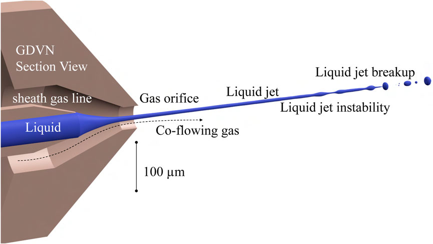
FIGURE 1. Gas-dynamic virtual nozzles (GDVNs) consist of gas focusing the liquid from the liquid line to a thin microjet. This jet experiences jet instability and eventually collapses into droplets.

In a typical XFEL experiment, GDVNs are operated with a helium mass flow rate of 30 mg/min and a liquid flow rate of 20 μL/min. The jet diameter is typically D ≈ 3 μm, and the jet speed is U ≈ 40 m/s (Knoška et al., 2020; Nazari et al., 2020). The Reynolds number for a water jet with viscosity μ ≈ 1 mPa⋅s and density ρ ≈ 1 g/cm³ is

$\text{Re}\equiv \frac{\rho UD}{\mu }\approx 120,(4)$

which suggests the dominance of inertial forces over viscous forces. While some samples in XFEL measurements are water-like, a great variety of liquid properties are possible with biological samples.

The initial formation of a jet requires inertial forces to overcome surface tension forces; the nozzle will otherwise produce drops or an unstable intermittent jet. This requirement is usually described by the Weber number

$\mathrm{W}\mathrm{e}=\frac{\rho U^{2}D}{2\sigma },(5)$

where σ is the surface tension of the liquid. In the case of a water-like sample in an XFEL measurement (σ ≈ 70 mN/m), the Weber number is approximately We ≈ 35. The transition from dripping to jetting occurs approximately when We ≳ 1, while Weber numbers that are too high lead to undesired lateral jet “whipping” behavior (Herrada et al., 2010).

An additional requirement to produce jets rather than drops is that the capillary number, defined as

$\text{Ca}=\frac{\mu U}{\sigma },(6)$

is sufficiently high. When the capillary number is too small, the jet breaks up too close to the meniscus (Vega et al., 2010). In a typical XFEL experiment with a water-like liquid, the capillary number is Ca ≈ 0.6.

The Ohnesorge number describes the ratio between viscous forces and surface tension force, and a typical value in an XFEL measurement for a water-like sample is

$\mathrm{O}\mathrm{h}=\frac{\mu }{\sqrt{\rho \sigma D}}=\frac{\sqrt{We}}{Re}\approx 0.06.(7)$

The collapse of a liquid jet is dictated by the Plateau–Rayleigh instability. Using the Laplace–Young equation and dimensional analysis, one can show that the critical time for collapse of a cylindrical column is proportional to the following parameter as summarized by Eggers and Villermaux (2008):

$t_c\propto \sqrt{\frac{\rho D^3}{\sigma }}.(8)$

This assumption ignores viscosity as a dominant force. Consequently, the jet length is proportional as shown in the following equation:

$L_c\propto U\sqrt{\frac{\rho D^3}{\sigma }}.(9)$

Further considerations by Gañán-Calvo et al. (2021) extend the aforementioned equations to include cases where viscosity may be dominant:

$L_c=\frac{\sigma }{\mathrm{\Delta }P}\frac{{\mathrm{W}\mathrm{e}}^2{\alpha }_{\rho }}{\left(\sqrt{{\mathrm{C}\mathrm{a}}^2{{\alpha }_{\mu }}^2+\mathrm{W}\mathrm{e}}-\mathrm{C}\mathrm{a}{\alpha }_{\mu }\right)}\approxeq {\alpha }_{\rho }U\sqrt{\frac{\rho D^3}{2\sigma }}\left(1+{\alpha }_{\mu }\frac{\mu }{\sqrt{\rho \sigma D}}\right),(10)$

where α_ρ and α_μ are dimensionless constants.

1.1.2 Navier–Stokes equations

The Navier–Stokes equations describe the temporal evolution of a fluid momentum vector field $(\rho \vec{U})$, which is the product of density (ρ) and velocity $(\vec{U})$:

$\frac{\partial }{\partial t}\left(\rho \vec{U}\right)+\nabla \cdot \left(\rho \vec{U}\otimes \vec{U}\right)-\nabla \cdot {\vec{\sigma }}_{\mu }=-\nabla p+{\vec{f}}_{\sigma }.(11)$

The viscous stress tensor $({\vec{\sigma }}_{\mu })$ for Newtonian fluids generalizes the molecular friction on continuum scales in terms of viscosity (μ):

$\overrightarrow{{\sigma }_{\mu }}=\mu \left(\nabla \vec{U}+{\left(\nabla \vec{U}\right)}^T\right)-\frac{2}{3}\mu \vec{I}\left(\nabla \cdot \vec{U}\right).(12)$

The density scalar ρ is transported along $\vec{U}$, and the mass-continuity equation is

$\frac{\partial \rho }{\partial t}+\nabla \cdot \left(\rho \vec{U}\right)=0.(13)$

We assume an incompressible flow, which renders $\vec{U}$ free of divergence:

$\nabla \cdot \vec{U}=0.(14)$

For ideal gases, the incompressible flow assumption typically holds when the Mach number is less than $\frac{1}{3}$ (Harlow and Amsden, 1968). For ideal gases, the Mach number can be defined as

$\mathrm{M}\mathrm{a}=\frac{|\vec{U}|}{c}=\frac{|\vec{U}|}{\sqrt{\gamma \bar{R}T}},(15)$

where c is the speed of sound, T is the temperature, $\bar{R}$ is the specific gas constant, and γ is the specific heat ratio. The surface tension force $({\vec{f}}_{\sigma })$ is in the direction of the normal pressure force of the interface. The surface tension force magnitude is proportional to the surface tension constant (σ) and the curvature (κ) of the interface and is only active at spatial coordinates where the interface is present $({\vec{x}}_f)$:

${\vec{f}}_{\sigma }=\sigma \kappa \widehat{n}\delta \left(\vec{x}-{\vec{x}}_f\right).(16)$

For our simulations of water jets with helium sheath gas, σ is assumed to be independent of the pressure and temperature of the fluid medium. Eqs 11, 13, and 14 end up forming five equations that are closed by five variables including $\vec{U}$, p, and ρ.

1.1.3 Volume-of-fluid method

The volume-of-fluid (VOF) method is a computational approach for describing immiscible interface on a finite volume grid illustrated in Figure 2. The immiscible interface is defined by the fraction of volume α that is occupied by the liquid phase within a given cell. A cell with α = 0 is completely occupied by gas, while a cell with α = 1 is completely occupied by liquid. The volume fraction dictates the density and viscosity at the interface cell according to the linear weighting

$\rho ={\rho }_{\text{liquid}}\alpha +{\rho }_{\text{gas}}\left(1-\alpha \right),(17)$

$\mu ={\mu }_{\text{liquid}}\alpha +{\mu }_{\text{gas}}\left(1-\alpha \right).(18)$

Assuming there is no evaporation and the flow is incompressible, the α field travels along the velocity field according to the advection equation:

$\frac{D\alpha }{Dt}=\frac{\partial \alpha }{\partial t}+\nabla \cdot \left(\vec{U}\alpha \right)=0.(19)$

This implies that the change in the volume fraction in a finite volume cell is equivalent to a flux of fluid passing through cell faces, according to the divergence theorem:

${\int }_{{\mathrm{\Omega }}_i}\frac{\partial \alpha }{\partial t}dV+{\int }_{\partial {\mathrm{\Omega }}_i}\alpha \vec{U}\cdot ndS=0.(20)$

FIGURE 2

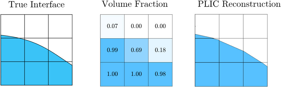
FIGURE 2. Illustration of volume-of-fluid and planar interface construction methods. Left: Description of a true liquid–gas interface. Center: Discrete cellular representation of volume of fluid, with numbers representing the fraction occupied by the liquid. Right: Discrete and piece-wise representation of continuous interface showing planar distribution of fluid fractions.

1.1.4 Planar interface construction (PLIC)

Advection with planar distribution is known for capturing interface physics more accurately than interface compression (Multidimensional Universal Limiter with Explicit Solution or MULES) methods (Gamet et al., 2020). In particular, OpenFOAM contains the isoAdvector solver, which takes advantage of geometric advection (Roenby et al., 2016). Before the advection, the volume fraction and velocity at the current time-step are known, and the goal is to compute α_i(t + Δt). The cell scalar α_i is described as such:

${\alpha }_i\left(t\right)=\frac{1}{|{\mathrm{\Omega }}_i|}{\int }_{{\mathrm{\Omega }}_i}\alpha \left(\vec{x},t\right)dV,(21)$

where Ω_i represents the volume inside cell i. For cells with 1 > α_i > 0, an interface known as the iso-face contains information about the distribution of liquid and gas within a cell. The planar equation describes this iso-face which is updated in every time-step. The values of the normal vector $\widehat{n}$ of this planar equation are computed using derivatives of the volume fraction field as

$\widehat{n}=\frac{\nabla \alpha }{\left|\nabla \alpha \right|}.(22)$

The Appendix contains a description of isoAdvector as described by Roenby et al. (2016).

1.1.5 Surface tension

Surface tension forces can be evaluated by ascertaining the interface curvature κ as

$\kappa =-\nabla \cdot \widehat{n}.(23)$

There are many approaches such as height functions to compute the curvature (Helmsen et al., 1997), which can be applied to Cartesian grids (Sussman, 2003). Using the height function approach to compute surface tension on non-Cartesian grids requires the need to populate the structured height function stencil with α from an unstructured grid to compute the curvature. This geometric interpolation adds to the computation cost (Ivey and Moin, 2015). Additionally, the most recent implementation of this on OpenFOAM only has support for structured grids (Saufi et al., 2020).

The default method setting for surface tension computation in OpenFOAM is continuum surface force (CSF) (Brackbill et al., 1992). This approach computes κ∇α, which is eventually used in the computation of ${\vec{f}}_{\sigma }$.

2 Numerical investigation of bell-shaped and cone-shaped nozzle designs

2.1 Gas-dynamic virtual nozzle geometry

We developed two different GDVN gas flow field geometries, namely, cone-shaped and bell-shaped, to investigate how the flow field geometry affects the liquid jet behavior. We additionally investigated how well the numerical simulations agree with experimental measurements. The geometries are shown in Figure 3 along with the design parameters and dimensional values. For our experimental comparisons, these designs were printed, developed, and assembled as described previously by Nazari et al. (2020). The complete nozzle design, including the channels that connect the gas and liquid lines to the nozzle, is shown in Figure 4.

FIGURE 3

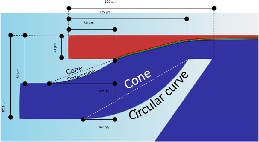
FIGURE 3. Geometry of the axis-symmetric cross-section of the cone- and bell-shaped nozzles. The circular curve geometry is used in the bell-shaped nozzles, while it is replaced by the straight line in the cone-shaped nozzle. The axis of symmetry is along the liquid jet (red). The inlets are shown on the left.

FIGURE 4

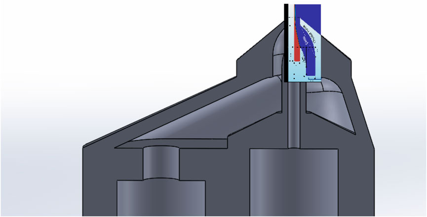
FIGURE 4. Geometry of the simulation superimposed on the sectioned view of the CAD of the manufactured GDVN.

The geometry and dimensions of the flow field domains used in the simulations were identical to the actual 3D-printed GDVN tips. The upstream bounds of the simulation flow field domains are shown in Figures 5, 6. The blue surfaces represent surfaces of mirror symmetry, and the domain is symmetric along this planar surface. The downstream flow field domains consisted of a concentric cylinder with a diameter of 1600 μm and length of 1100 μm, as shown in Figure 7. A 3D half geometry was made for the flow field domain representation to save computation time since the GDVN flow fields are symmetrical along the jet propagation axis.

FIGURE 5

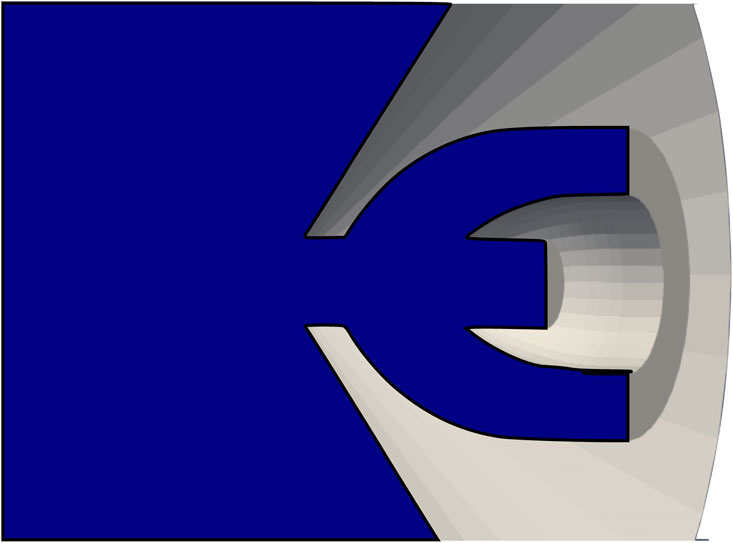
FIGURE 5. Computational flow field for the GDVN with bell-shaped geometry for the gas flow field. Blue surface represents the surface of symmetry.

FIGURE 6

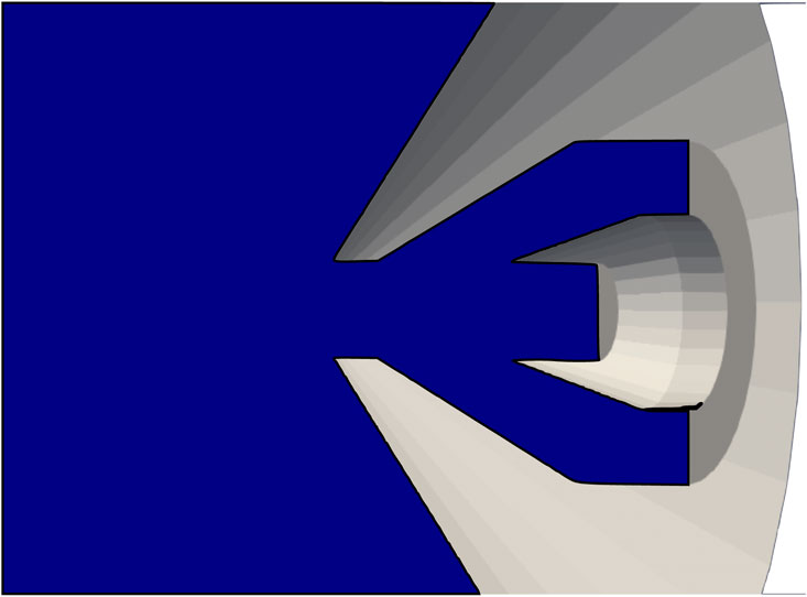
FIGURE 6. Computational flow field region for the GDVN with cone-shaped geometry for the gas flow field.

FIGURE 7

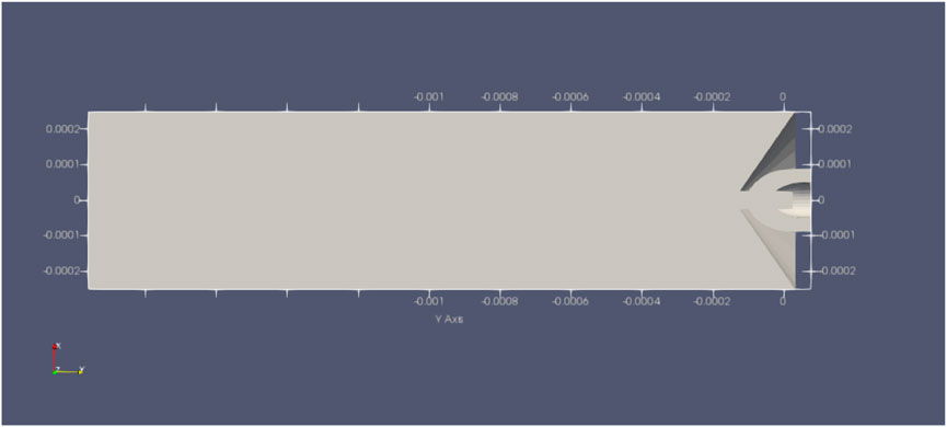
FIGURE 7. Complete flow field region for the bell-shaped nozzle numerical simulation.

2.2 Experimental testing and numerical simulation

For both the numerical simulation and experimental testing, the inlet boundary condition for the liquid is the inlet volumetric flow rate, which was set to a value of 48 μL/min, and the liquid was pure water. The sheath gas was helium, and the flow rate was set to 6 mg/min.

The Euler method was the implicit integration scheme used to advance the simulation in time. The method used for advection of velocity was linear upwind. A linear scheme was used to evaluate the viscous terms. This is discussed more in detail in supplemental material.

The total mesh count of the cone- and bell-shaped nozzle domains was approximately 100,000 grid points without adaptive mesh refinement (AMR). The mesh count for a fully developed jet that is set to three AMR levels increased to approximately 9 million grid points for both the cone- and bell-shaped GDVN simulations. The simulation time would increase 16-fold if the mesh resolution was doubled. This is because each hexahedral cell would be subdivided into eight cells, and the number of temporal time-steps would also double to satisfy the CFL condition and reduce temporal discretization errors (Courant et al., 1967). With AMR, the assumption is that the resolution is more than enough to capture viscous scales, but areas near the interface require more refinement to capture interface dynamics. As such, the refinement only occurs near the interface. This results in the simulation time scaling proportional to 2³ instead of 2⁴. Based on the incompressible flow assumption, the velocity at the nozzle can be computed using the mass conservation equation, where the mass flux and volume flux are constant from the inlet of gas to the orifice. The velocity was computed based on our geometry and 6 mg/min. As a result, we ascertain the average velocity to be 286 m/s, which is less than 0.3 Mach. Therefore, we can conclude that the incompressible assumption for the operating condition is valid.

2.3 Simulation runs

For the test case, the Mach number is calculated as less than 0.3 for the sheath gas to assume that the flow is incompressible. Furthermore, the domain of the large half-cylinder that accounts for the chamber of the flow field region of the bell-shaped case and the cone-shaped case is designed to be big enough so that the influence of outlet boundary conditions on the upstream flow would be negligible. The mean jet length values of the simulation runs are shown in Table 1.

TABLE 1

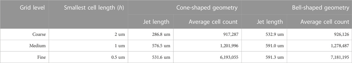
TABLE 1. Mean jet-length values inside the domain with three different AMR grid levels. The value h indicates the finest resolution at the interface after AMR.

2.4 Adaptive mesh refinement to improve simulation accuracy while preserving high runtime efficacy

Adaptive mesh refinement is a technique to improve the accuracy of interface dynamics and advection since it refines the resolution of the computational mesh at and around the interface. When we undergo a mesh refinement level, the cell sizes are refined by a factor of two in the vicinity of the liquid–gas interfaces. The refinement in a given cell i is activated based on a volume fraction criterion 0.999 < α_i < 0.001. The refinement is recursive until desired levels of refinements are achieved. A more detailed description is shown in Appendix. Figure 8 shows the cross section of the cases for three different mesh resolutions for the cone-shaped nozzle, namely, one-level AMR, two-level AMR, and three-level AMR. Numerical errors are expected to be comparatively the highest in the case with one-level AMR (the left picture of Figure 8). Undesirable asymmetry is noticed in this case in part due to those errors. However, with increased adaptive refinement levels, the effect of truncation errors in numerical simulation becomes less prominent. We performed simulations with adaptive mesh refinements of three levels to achieve the highest possible accuracy for the results while keeping the computation costs low.

FIGURE 8

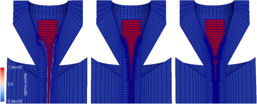
FIGURE 8. Grid resolution independence study for the numerical simulation test case of the bell-shaped nozzle. The left picture corresponds to one-level AMR without global mesh refinement (coarsest mesh resolution in the vicinity of the liquid–gas interface), the middle picture corresponds to two-level AMR (medium mesh resolution in the vicinity of the liquid–gas interface), and the right picture corresponds to three-level AMR (fine mesh resolution in the vicinity of the liquid–gas interface).

The solutions to jet-length mean come by averaging fluctuating jet length over time. However, the true mean cannot be reflected by sampled data over a short span of time, which could explain why the convergence order is inconsistent between the cone and the bell. The convergence order of 7 reflects that conclusion. It would be fruitful to compare simulation results with the experimental data.

2.4.1 Parallelization

OpenFOAM codes are based on MPI (message-passing interface) multithreading (Walker (1992)) to ensure OpenFOAM’s versatility over shared memory and distributed memory architectures. The Agave HPC (high-performance computing) facility of Arizona State University was used to run the numerical simulations which comprises several 100 nodes with 28 cores. The computational efficiency of the simulations is greatly enhanced when run on a single node due to localized communication. Most of the computations conducted are on a single node. However, the simulations with the highest resolution require a higher number of nodes, and as such, the computation is conducted over distributed memory.

The “Simple method” in OpenFOAM executes a grid decomposition of the domain. It varies the domain boundaries such that the computational load that depends on the number of cells is equivalently distributed. The “Simple Method” should not be confused with the SIMPLE algorithm for advancing the fluid simulation. The “Scotch method” distributes an equal amount of cell count over multiple cores while minimizing the number of cells at the boundary of the domain of each core. For example, Figure 9 showing how the computational domain corresponding to the bell-shaped nozzle is decomposed to run on 16 cores be the aforementioned “Simple” method, and Figure 10 showing how the computational domain corresponding to the bell-shaped nozzle is decomposed to run on 16 cores be the aforementioned “Scotch” method. The Scotch decomposition enables the distribution of all the domains’ cells across multiple nodes and cores. The Scotch algorithm minimizes the number of contact cells while also minimizing the difference in the number of cells for each processor.

FIGURE 9

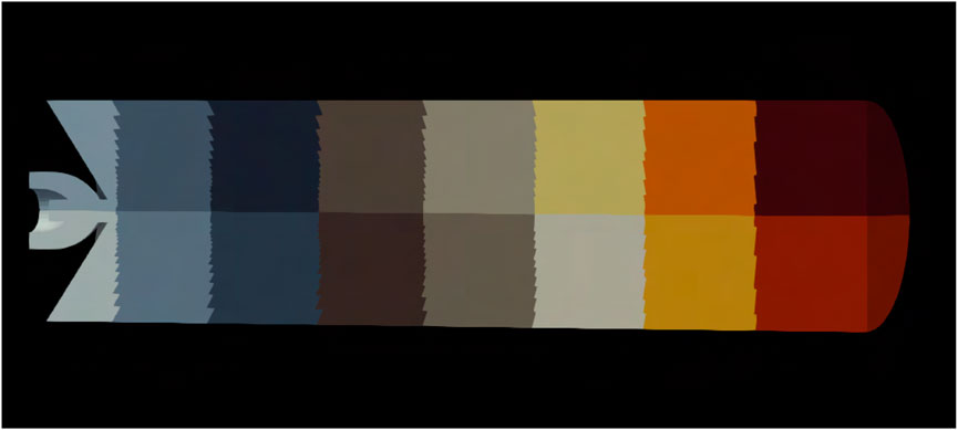
FIGURE 9. Computational geometry section distributed across different processors according to the Simple domain decomposition strategy.

FIGURE 10

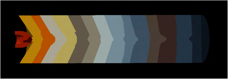
FIGURE 10. Computational geometry section distributed across different processors according to the Scotch domain decomposition strategy.

In numerical experiments, we ascertained that the “Scotch method” performed faster than the “Simple method” as evidenced in Figure 11. This is likely because the “Simple method” is restricted to cuboid-shaped partitions that do not allow for equal numbers of cells in each domain. One can also see that an increase in the number of cores does not necessarily cause an increase in speed, likely because of the MPI sending and receiving overheads and the spreading of computations across different compute nodes.

FIGURE 11

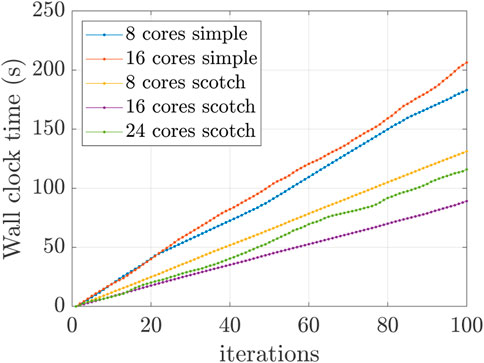
FIGURE 11. Domain decomposition strategies and their computation speeds. The “Scotch method” performs better than the “Simple method.”

For the highest resolution, the simulation ran for 7 days with 108 cores. This resulted in the utilization of roughly 18,000 core hours. The biggest bottleneck in the simulations is the CFL condition for cells in the finest part of the mesh. While the momentum equation solution allows for the CFL condition to exceed 1, the geometric advection of the interface is restricted to less than 0.5. An improvement that could be made to the simulation is automatic load balancing. As the simulation runs on multiple cores, the number of cells in each computational core keeps changing due to AMR. Because of the lack of implementation of load balancing in the current OpenFOAM version 1906, load balancing could only be performed manually by stopping the simulation, reconstructing the mesh, decomposing it again, and then continuing the run.

2.5 Microjet imaging and analysis

The microjet data collection and analysis procedures were equivalent to those described in our previous publication (Nazari et al., 2020), except that the measurements were made at atmospheric pressure in this study. The liquid volumetric flow rate was controlled using a high-pressure liquid chromotography (HPLC) pump (Shimadzu LC-20AD), which also monitored liquid pressure. The helium mass flow rate was controlled using a mass flow controller (Bronkhorst EL-FLOW). Images were recorded using a CMOS camera (Photron SA5) along with a ×10 long-working-distance objective (Mitutoyo ×10 M Plan Apo) and an adjustable 0.58–7 zoom lens (Navatar 12X UltraZoom) at a frame rate of 100 Hz. A double-pulsed fiber-coupled 100-ns laser at 633 nm wavelength (DILAS D4F4S22 laser with custom pulsed current driver) illuminated the jet.

The data processing scheme is described in Nazari et al. and consisted of image filtering, thresholding, and segmentation as shown in Figure 12. The distance from the nozzle tip to the end of the longest contiguous segment, where the first droplet detaches from the jet, was taken as our measure of jet length. A jet length was determined from each image and the statistics compiled as discussed in Section 2.6.

FIGURE 12

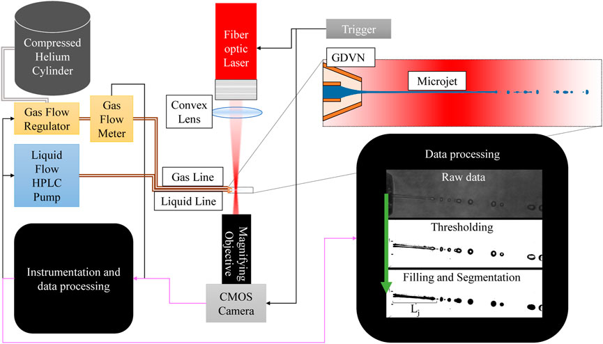
FIGURE 12. Schematic of the microjet imaging setup. The double lines represent fluid flow, black lines represent electronic communications, and magenta lines represent image data. The gas flow regulator/meter controls the mass flow rate of helium to the GDVN. The HPLC pump controls the volumetric flow rate of the liquid to the GDVN. A fiber-coupled nanosecond laser is focused near the GDVN, which is imaged using a CMOS camera. The data processing steps illustrated in the black box include image filtering, thresholding, and segmentation.

When operating a GDVN with an HPLC pump, the accuracy of the volumetric flow rate is approximately 15%, which we determined by comparing against a Sensirion SLI-0430 flowmeter, and also by measuring the mass of dispensed water. Typical fluctuations of approximately 5% are observed, with a frequency corresponding to that of the pump pistons. The timescale of these fluctuations are approximately 0.1 Hz, which is far too long to cause jet instabilities. We confirmed the presence of flow fluctuations by measuring with two liquid flowmeters in parallel, and we observed fluctuations in two different HPLC devices of the same model (Shimadzu LC-20AD). The liquid flow fluctuations are significantly larger than the expected 0.1% accuracy. The gas mass flow rate accuracy and repeatability is approximately 2% and 0.2%, respectively, as per the vendor’s specifications. We confirmed the specified accuracy by capturing gas bubbles in a graduated cylinder and measuring volumetric displacement. The maximum resolution of the optical system is approximately 1.1 μm, due to the numerical aperture of 0.28. This puts the jet length measurement precision less than 1% even with digital image processing artifacts considered.

2.6 Simulation results and comparison to experiments

Figure 13 shows the results of the transient jet length from the simulation run of the highest resolution. The jet length increases consistently with the slope equaling the jet speed until it collapses and resets to a lower value. The jet lengths were ascertained from simulation data by taking jet profiles at every microsecond time-step. The longest contiguous segment of the microjet from the orifice was taken to be the jet length. Figure 14 shows the comparison of jet-length histograms of the bell-shaped and cone-shaped geometries, while Figure 15 shows the comparison of the histograms of simulations against the experiment. Figure 16 shows the boxplots of experimental results for different printed nozzles. Figures 15A, B, 16A, B show the comparison of the experimental results and the numerical simulation results for the cone-shaped nozzle and the bell-shaped nozzle running under similar operating conditions. We compared the simulations to experiments by these histograms. They show the distribution of jet length by characterizing its probability density for various bins of jet lengths. These jet lengths captured transient evolution of the jet in simulation and experiment.

FIGURE 13

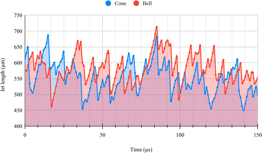
FIGURE 13. Transient evolution of the jet length for cone- and bell-shaped geometry ascertained from two-phase flow simulation.

FIGURE 14

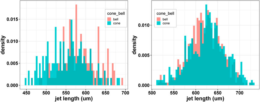
FIGURE 14. Numerical simulation results of the cone-shaped and bell-shaped nozzles (left) and experimental results of the cone-shaped and bell-shaped nozzles (right). The operating conditions are 48 μL/min for the liquid (water) flow rate and 6 mg/min for the sheath gas flow rate.

FIGURE 15

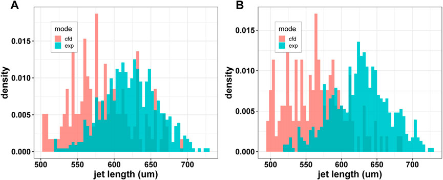
FIGURE 15. Experimental and CFD results of the bell-shaped nozzles (A) and experimental and CFD results of the cone-shaped nozzles (B). The operating conditions are 48 μL/min for the liquid (water) flow rate and 6 mg/min for the sheath gas flow rate.

FIGURE 16

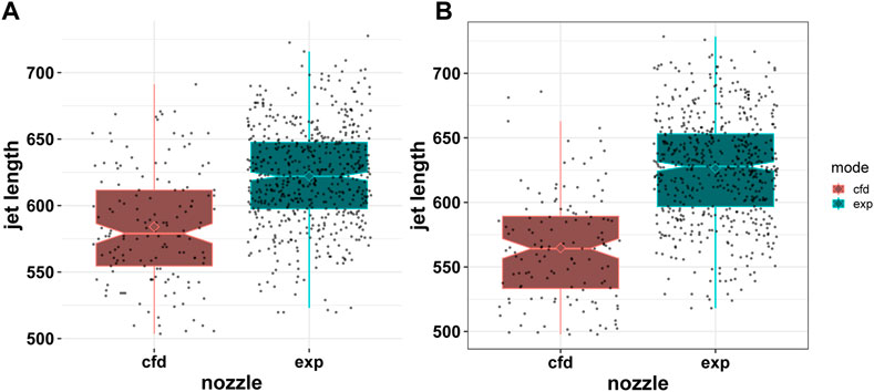
FIGURE 16. Boxplot of experimental and CFD results of the bell-shaped nozzles (A) and boxplot of experimental and CFD results of the cone-shaped nozzles (B). The operating conditions are 48 μL/min for the liquid (water) flow rate and 6 mg/min for the sheath gas flow rate.

Figure 15A shows the simulation results of the jet length values for the time-steps between 850 μs and 1000 μs. The data show that the bell-shaped nozzle generally results in a slightly longer mean liquid jet length value under the same operating conditions. Quantitatively, the mean value for the jet length result of the bell-shaped nozzle (582 μm with a standard deviation of 44 μm) is about 5% longer than the corresponding value for the cone-shaped nozzle (553 μm with a standard deviation of 49 μm). On the other hand, Figure 14B shows the experimental results from the three cone-shaped and bell-shaped 3D-printed nozzles. Experimental results are obtained using the test station and imaging and image processing pipeline explained in our previous paper (Nazari et al., 2020). The experimental setup is shown in Figure 12. As for the experimental result’s data for the three cone-shaped nozzles and the three bell-shaped nozzles, the bell-shaped nozzle results in a slightly shorter mean liquid jet length. The mean value for the experimental jet length results of the bell-shaped nozzle (622 μm) with a standard deviation of 37 μm is about 1% shorter than the corresponding value for the cone-shaped nozzle (626 μm) with a standard deviation of 42 μm.

Figures 15A, B show the histograms of jet length values of experimental observations (three bell-shaped nozzles and three cone-shaped nozzles) versus the results of numerical simulations for the cone-shaped nozzle and the bell-shaped nozzle. The data in Figure 15A show that the mean jet-length value in the numerical simulation is about 1% larger than the mean jet-length value in the experimental result for the bell-shaped nozzle. However, the mean value of the CFD results is about 10% larger than the corresponding values of the experimental results for the cone-shaped nozzle.

Figures 16A, B show the boxplot of the jet-length values from experimental data of three nozzles of same geometry versus CFD results for the bell-shaped design and the cone-shaped design, respectively. In the figures, the diamonds show the mean value for each case, the black dots show the jet-length value, the red points show the outliers, and the horizontal lines of the boxplots represent the quartiles of the jet length. Figure 16 shows that the numerical simulation underestimates the jet length by about 6% for the bell-shaped geometry and underestimates the mean jet-length value by about 12% for the cone-shaped geometry.

Figures 17A, B show the boxplot of jet lengths of the experimental data taken from three bell-shaped nozzles and three cone-shaped nozzles, respectively. The three nozzles are of same type each with manufacturing inaccuracies from the SLA printing process. For jet-length data of the bell-shaped nozzles, the mean value of nozzle 1 is 632 μm and the standard deviation value is 41 μm. For nozzle 2 of bell-shaped nozzles, the mean jet length is 621 μm and the standard deviation is 50 μm. Finally, for nozzle 3 of the bell-shaped nozzles, the mean jet length is 595 μm and the standard deviation is 47 μm. On the contrary, for experimental data for the jet length of the cone-shaped nozzles, nozzle 1 has a mean value of 632 μm and a standard deviation of 50 μm. Nozzle 2 of the cone-shaped nozzles has a mean jet length of 635 μm and a standard deviation of 61. Finally, nozzle 3 of the cone-shaped nozzles has a mean jet length of 591 μm and a standard deviation of 43 μm.

FIGURE 17

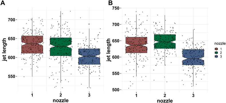
FIGURE 17. Boxplot of experimental results of three bell-shaped nozzles (A) and boxplot of experimental results of three cone-shaped nozzles (B).

Figure 18 shows the boxplot of experimental results for jet lengths of five cone-shaped nozzles. For the experimental results of the jet lengths of the cone-shaped nozzles, nozzle 1 has a mean value of 635 μm and a standard deviation of 61 μm; nozzle 2 has a mean value of 646 μm and a standard deviation of 54 μm; nozzle 3 has a mean value of 666 μm and a standard deviation of 52 μm; nozzle 4 has a mean value of 662 μm and a standard deviation of 60 μm; and nozzle 5 has a mean value of 653 μm and a standard deviation of 50 μm.

FIGURE 18

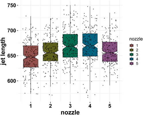
FIGURE 18. Boxplot of experimental results for jet lengths of five cone-shaped nozzles.

The integrated plots show the CFD results versus the experimental results in Figures 15A, B. Reynold’s number can be expressed as a function of the mass flow rate $(\dot{m})$ or volumetric flow rate (Q):

$\mathit{R}\mathit{e}=\frac{4\dot{m}}{\pi D\mu }=\frac{4\rho Q}{\pi D\mu }.(24)$

Given the known values of all other properties of the liquid and the gas, we ascertain that Reynold’s number for liquid flow is around 20 in the liquid line and exceeds to around 100 as it becomes a jet. Reynold’s number of the gas flow at the nozzle tip is around 25. Under such conditions, we can expect the flow near the nozzle tip to be hydrodynamically stable. We have ascertained that the HPLC pump used had an inaccuracy of about 10%–20%. This is the most likely explanation for the mismatch between CFD and experimental results. Additionally, the adaptive mesh refinement could have introduced tiny numerical perturbation which causes the jet to collapse prematurely but does not significantly reduce the jet length. This would occur due to the refinement criterion of 0.001 ≤ α ≤ 0.999. The cells in this range are refined, but the cells outside this range are not refined, creating a few cells that have a small amount of interface that are not refined as per the criterion. This would add noise to the curvature field resulting in the numerical perturbations described previously. Another possible reason for the discrepancy is that the atmosphere is simulated as a helium atmosphere, while in the experiment, the GDVN expels the microjet into the ambient air. While it was assumed that the Plateau–Rayleigh breakup of the jet is not influenced by the type of atmosphere, the reduced inertia of the surrounding gas could have reduced resistance to the jet breakup, contributing to the decrease in ascertained jet lengths from the CFD results in comparison to the experimental data.

2.7 Contours and figures from the numerical simulation results

Details about the numerical simulation results are shown in this section. Figure 19 shows the pressure contours in pascal for the 3D simulation of the cone-shaped design and the bell-shaped design. The figure shows a pressure drop from inside the nozzle to outside. This pressure gradient drives the gas out at high subsonic velocities. Additionally, a pressure jump is seen at the free surface along the microjet. The surface tension force causes this pressure jump, and hence it is a sharp pressure jump. The pressure jump is about 150 mbar and corresponds to a jet diameter of about 9 microns. The liquid line is under the highest amount of pressure. The cone nozzle produces a marginally smaller pressure inside the nozzle.

FIGURE 19

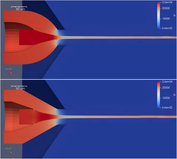
FIGURE 19. Image shows the numerical simulation at a random time-step alongside a random snapshot of the experimental testing of a running jet from the cone-shaped GDVN. For comparison, the two snapshots were chosen to have matching jet lengths; this is not an indication of matching mean jet lengths between numerical and experimental results.

Streamlines of the flow field are shown in Figure 20. Re-circulation cells are also shown in Figure 20. This re-circulation is caused by shear stress on the liquid by the gas inside the nozzle. The shear stress accelerates the liquid near the free surface, which drives an inverted vortex ring along the mouth of the liquid line. The back-flow in the vortex occurs as a result of continuity enforcement. The cone and bell shapes of the nozzles have a visible impact on the shape of the re-circulation. Additionally, the nozzles focus on the streamlines toward the orifice. The gas is accelerated due to a reduced cross-sectional area as the gas approaches the orifice. The liquid accelerates due to the shear all along the free surface from the gas. The shear is roughly understood as the gradient of velocity magnitude perpendicular to the streamlines.

FIGURE 20

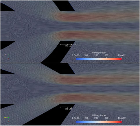
FIGURE 20. Pressure scalar field in pascals for the gas and liquid for the 3D simulation of the cone-shaped and bell-shaped nozzles. The pressure drop from inside the nozzle and outside is responsible for the gas acceleration at the orifice. The pressure jump inside the liquid jet occurs as a result of surface tension.

AMR for the cells in the vicinity of the liquid–gas interface is shown in Figure 21. Contours for the velocity magnitude (in m/s) in the direction of the jet are shown in Figure 22. AMR levels can be seen for the cells that are in the vicinity of the liquid–gas interface.

FIGURE 21

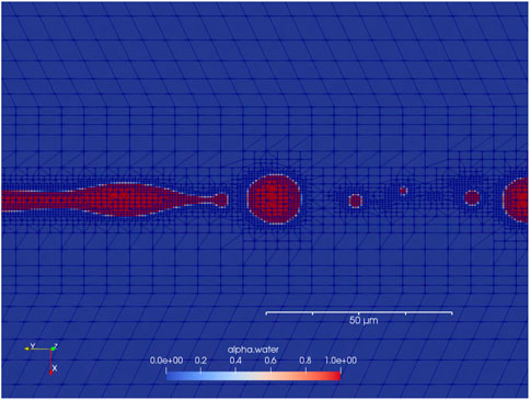
FIGURE 21. Visualization of the Plateau–Rayleigh instability of the microjet ascertained from simulation data. The simulation shows the dynamic computational grid with three AMR levels for the cells in the vicinity of the liquid–gas interface for the bell-shaped nozzle design.

FIGURE 22

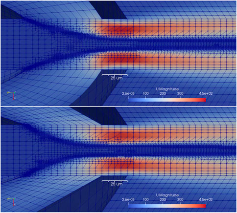
FIGURE 22. Streamlines of the gas flow and the liquid flow for the 3D simulation of the cone-shaped and the bell-shaped nozzle designs. The streamlines are visualized by a noise function motion blurred in the direction of the velocity with the contours representing the magnitude of the velocity.

A cross section of the jet and how it breaks up into droplets is shown in Figure 23.

FIGURE 23

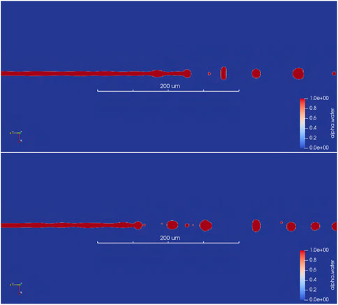
FIGURE 23. Simulation generated magnitude of the velocity vector field in m/s along with the dynamic computational grid around the orifice of the GDVN. This negative y-direction is the direction of jet propagation.

The jet regions for a running nozzle along with the droplets after the jet breakup for the whole flow field are shown in Figure 24 for the cone-shaped and the bell-shaped designs. Near the jet breakup, several satellite droplets are visible, caused by ligamentation column collapse. These smaller satellite droplets disappear with higher drag acceleration and merge with a larger droplet ahead of them. Another consequence of ligamentation is droplet oscillation resulting in initially deformed droplets right after the breakup, damping down to a circular-shaped downstream. The oscillation profile is a function of the Weber number. It occurs due to surface tension force acting as restoring force and tending the droplet toward a spherical shape. The momentum created by this force creates an oscillatory motion that is dampened by the viscosity of water. The aforementioned forces are analogous to a spring-mass system, where the spring force is equivalent to the surface tension force while the viscosity is equivalent to the friction.

FIGURE 24

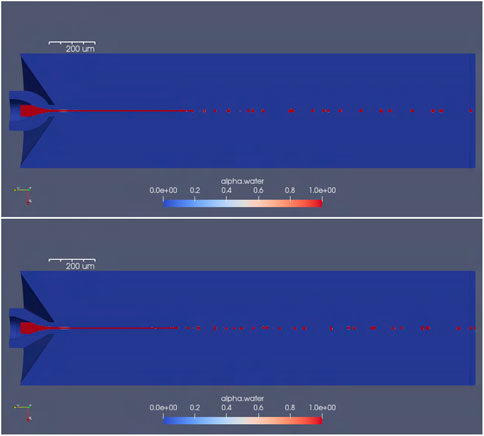
FIGURE 24. Cross section of the jet and how it breaks up into droplets for the bell-shaped design (upper picture) and the cone-shaped design (lower picture).

Reynold’s number of the microjet ascertained numerically and experimentally can also be expressed as a function of the mass flow rate $(\dot{m})$ or volumetric flow rate (Q):

$\mathit{R}\mathit{e}=\frac{4\dot{m}}{\pi D\mu }=\frac{4\rho Q}{\pi D\mu }.(25)$

Given the known values of all other properties of the liquid and the gas, we ascertain that Reynold’s number for liquid flow is around 20 in the liquid line and exceeds to around 100 as it becomes a jet. Reynold’s number of the gas flow at the nozzle tip is around 25. Under such conditions, we can expect the flow near the nozzle tip to be hydro-dynamically stable.

3 Conclusion

We were able to generate a pipeline to simulate GDVN microfluidics in the incompressible regime with OpenFOAM open-source software and with the help of the online community associated with it. We were able to simulate the medium resolution of the simulation with only 16 cores in 1 week. The simulations were conducted with adaptive mesh refinement, which reduced the number of cells by 95% from global mesh refinement. We used a structured hex mesh instead of unstructured hex-dominant mesh or unstructured tet-mesh to facilitate AMR usage. Our structured hex cell could be equivalent to about six tetrahedral cells. This pipeline enables us to look at the fluid phenomenon that is not explicitly axis-symmetric such as whipping. The cone- and bell-shaped nozzles show quantitative agreement with experimental data with a relative error of about 10%. On the other hand, the GCI analysis shows qualitative convergence but lacks quantitative convergence due to monotonic convergence. There is an insufficient resolution range to achieve the dominant error in spatial discretization from a single Taylor expansion. The other possibility is the lack of enough data to reduce the uncertainty in the true mean, which creates a lot more uncertainty. The same pipeline can be expanded to a compressible regime to simulate GDVN microfluid jet dynamics with a high gas flow rate. In addition, a non-conformal mesh helps form more complex geometries that cannot be easily refined using multi-block meshes.

Data availability statement

The raw data supporting the conclusion of this article will be made available by the authors, without undue reservation.

Author contributions

The authors confirm contribution to the paper as follows: study conception and design: RN, AA, MH, RA, and RK; data collection: RN, AA, and RK; analysis and interpretation of results: RN, AA, MH, RA, and RK; draft manuscript preparation: RN, AA, MH, RA, and RK. All authors reviewed the results and approved the final version of the manuscript.

Funding

This research was funded by the National Institutes of Health (1S10OD021816), National Science Foundation BioXFEL Science and Technology Center (1231306), and the National Science Foundation (1817862 and 1943448).

Acknowledgments

The authors thank Professor John Spence, Professor Kevin Schmidt, Joe Chen, Konstantinos Karpos, Roberto Alvarez, and Sahba Zaare of the Physics Department of Arizona State University for fruitful discussions and technical assistance for the experiments. The authors also thank Research Computing at Arizona State University for providing HPC and storage resources that have contributed to the research results reported within this paper.

Conflict of interest

The authors declare that the research was conducted in the absence of any commercial or financial relationships that could be construed as a potential conflict of interest.

Publisher’s note

All claims expressed in this article are solely those of the authors and do not necessarily represent those of their affiliated organizations, or those of the publisher, the editors, and the reviewers. Any product that may be evaluated in this article, or claim that may be made by its manufacturer, is not guaranteed or endorsed by the publisher.

References

Brackbill, J. U., Kothe, D. B., and Zemach, C. (1992). A continuum method for modeling surface tension. J. Comput. Phys. 100, 335–354. doi:10.1016/0021-9991(92)90240-y

CrossRef Full Text | Google Scholar

Courant, R., Friedrichs, K., and Lewy, H. (1967). On the partial difference equations of mathematical physics. IBM J. Res. Dev. 11, 215–234. doi:10.1147/rd.112.0215

CrossRef Full Text | Google Scholar

DePonte, D., Weierstall, U., Schmidt, K., Warner, J., Starodub, D., Spence, J., et al. (2008). Gas dynamic virtual nozzle for generation of microscopic droplet streams. J. Phys. D Appl. Phys. 41, 195505. doi:10.1088/0022-3727/41/19/195505

CrossRef Full Text | Google Scholar

Eggers, J., and Villermaux, E. (2008). Physics of liquid jets. Rep. Prog. Phys. 71, 036601. doi:10.1088/0034-4885/71/3/036601

CrossRef Full Text | Google Scholar

Gamet, L., Scala, M., Roenby, J., Scheufler, H., and Pierson, J.-L. (2020). Validation of volume-of-fluid openfoam® isoadvector solvers using single bubble benchmarks. Comput. Fluids 213, 104722. doi:10.1016/j.compfluid.2020.104722

CrossRef Full Text | Google Scholar

Gañán-Calvo, A. M., Chapman, H. N., Heymann, M., Wiedorn, M. O., Knoska, J., Gañán-Riesco, B., et al. (2021). The natural breakup length of a steady capillary jet: Application to serial femtosecond crystallography. Crystals 11, 990. doi:10.3390/cryst11080990

CrossRef Full Text | Google Scholar

Gañán-Calvo, A. M. (1998). Generation of steady liquid microthreads and micron-sized monodisperse sprays in gas streams. Phys. Rev. Lett. 80, 285–288. doi:10.1103/physrevlett.80.285

CrossRef Full Text | Google Scholar

Harlow, F. H., and Amsden, A. A. (1968). Numerical calculation of almost incompressible flow. J. Comput. Phys. 3, 80–93. doi:10.1016/0021-9991(68)90007-7

CrossRef Full Text | Google Scholar

Helmsen, J., Colella, P., and Puckett, E. G. (1997). Non-convex profile evolution in two dimensions using volume of fluids. Tech. rep. Lawrence Berkeley Lab., CA (United States).

Google Scholar

Herrada, M. A., Ferrera, C., Montanero, J. M., and Gañán-Calvo, A. M. (2010). Absolute lateral instability in capillary coflowing jets. Phys. Fluids 22, 064104. doi:10.1063/1.3447800

CrossRef Full Text | Google Scholar

Ivey, C. B., and Moin, P. (2015). Accurate interface normal and curvature estimates on three-dimensional unstructured non-convex polyhedral meshes. J. Comput. Phys. 300, 365–386. doi:10.1016/j.jcp.2015.07.055

CrossRef Full Text | Google Scholar

Knoška, J., Adriano, L., Awel, S., Beyerlein, K. R., Yefanov, O., Oberthuer, D., et al. (2020). Ultracompact 3d microfluidics for time-resolved structural biology. Nat. Commun. 11, 657–669. doi:10.1038/s41467-020-14434-6

PubMed Abstract | CrossRef Full Text | Google Scholar

Nazari, R., Zaare, S., Alvarez, R. C., Karpos, K., Engelman, T., Madsen, C., et al. (2020). 3d printing of gas-dynamic virtual nozzles and optical characterization of high-speed microjets. Opt. Express 28, 21749–21765. doi:10.1364/oe.390131

PubMed Abstract | CrossRef Full Text | Google Scholar

Roenby, J., Bredmose, H., and Jasak, H. (2016). A computational method for sharp interface advection, R. Soc. open Sci. 3, 160405. doi:10.1098/rsos.160405

PubMed Abstract | CrossRef Full Text | Google Scholar

Saufi, A. E., Desjardins, O., and Cuoci, A. (2020). An accurate methodology for surface tension modeling in openfoam. arXiv preprint arXiv:2005.02865

Google Scholar

Scheufler, H., and Roenby, J. (2019). Accurate and efficient surface reconstruction from volume fraction data on general meshes. J. Comput. Phys. 383, 1–23. doi:10.1016/j.jcp.2019.01.009

CrossRef Full Text | Google Scholar

Sussman, M. (2003). A second order coupled level set and volume-of-fluid method for computing growth and collapse of vapor bubbles. J. Comput. Phys. 187, 110–136. doi:10.1016/s0021-9991(03)00087-1

CrossRef Full Text | Google Scholar

Sutton, G. P., and Biblarz, O. (2016). Rocket propulsion elements. United States: John Wiley and Sons.

Google Scholar

Vega, E. J., Montanero, J. M., Herrada, M. A., and Gañán-Calvo, A. M. (2010). Global and local instability of flow focusing: The influence of the geometry. Phys. Fluids 22, 064105. doi:10.1063/1.3450321

CrossRef Full Text | Google Scholar

Walker, D. W. (1992). Standards for message-passing in a distributed memory environment. TN (United States): Tech. rep., Oak Ridge National Lab.

Google Scholar

Wörner, M. (2012). Numerical modeling of multiphase flows in microfluidics and micro process engineering: A review of methods and applications. Microfluid. nanofluidics 12, 841–886. doi:10.1007/s10404-012-0940-8

CrossRef Full Text | Google Scholar

Zahoor, R., Bajt, S., and Šarler, B. (2018a). Influence of gas dynamic virtual nozzle geometry on micro-jet characteristics. Int. J. Multiph. Flow 104, 152–165. doi:10.1016/j.ijmultiphaseflow.2018.03.003

CrossRef Full Text | Google Scholar

Zahoor, R., Bajt, S., and Šarler, B. (2018b). Numerical investigation on influence of focusing gas type on liquid micro-jet characteristics. Int. J. Hydromechatronics 1, 222–237. doi:10.1504/ijhm.2018.092732

CrossRef Full Text | Google Scholar

Zahoor, R., Regvar, R., Bajt, S., and Šarler, B. (2020). A numerical study on the influence of liquid properties on gas-focused micro-jets. Prog. Comput. Fluid Dyn. Int. J. 20, 71–83. doi:10.1504/pcfd.2020.106407

CrossRef Full Text | Google Scholar