LQR and LQG-Kalman active control comparison of smart structures with finite element reduced-order modeling and a Monte Carlo simulation

The present contribution presents a comparison between two types of controls, namely, the optimal linear quadratic regulator (LQR) and the Kalman-LQG controller using the model order reduction process. Due to numerical constraints, the models of structures have been reduced so that the design of controllers and/or estimators could be performed. The proposed method results in a significant reduction in computational costs for dynamic analysis without compromising on accuracy. Transforming the full order state-space resulting from finite element space to a lower model reduces the simulation time with a few degrees of freedom and helps to implement easily the control without changes in the dynamics of the structure. The estimator Kalman is used here in order to estimate the modal states of the system that are used in modal analysis. In this context, a one-side cantilever Timoshenko beam is chosen with perfectly bonded piezoelectric layers of actuators and sensors to apply this comparison. The Monte Carlo simulation was used to improve the number and location selection of piezoelectric sensors on the chosen beam model. Neglecting environmental effects, numerical results relating to this comparison without and with model order reduction are established. Simulation results are presented to illustrate the effectiveness of the proposed vibration control algorithm for the studied beam.

1 Introduction

The model order reduction (MOR) process, also called the reduced order model (ROM), is studied and used in many fields of engineering and mathematics. More precisely, it is used to reduce the computational cost and the complexity of computations in modeling and control of structures without changes in their accuracy. Mathematically, the concept of reduced models is developed from solving eigenvalue problems that require a considerable amount of computation. It would be very helpful to reduce the size of the model while keeping the accuracy of eigenvalues and vectors.

A wide range of methods, concerning linear and nonlinear models of reduction, has been reported in the literature. For example, modal and balanced truncations have been investigated for linear models and orthogonal decomposition by Hughes and Skelton (1981) and Willcox and Peraire (2002). The principal component analysis is analyzed for nonlinear models by Hsieh (2002). The balanced truncation presented by Willcox and Peraire (2002) and Hsieh (2002) has used the snapshot matrix for singular decomposition that is not appropriate with the matrices of full models. Another frequently used model reduction technique in linear structural dynamics, investigated by Callahan et al. (1989), is the system equivalent reduction expansion process (SEREP), which also allows for the preservation of the modes and dynamics of the model. It is this last technique that will be used in this study because of its adaptation to all types of structures.

Regarding the control procedure, increasing the order of the system increases the order of the controller. A relatively high order of the controller is complicated to design because of a large number of states and can cause system instability. The LQR control requires the measurement of all state variables, while in the linear quadratic Gaussian LQG controller, this measurement of all states is not necessary. The LQG-Kalman design is implemented by combining the optimal regulator and the Kalman filter in one optimal controller/estimator to obtain the estimated state of the input vector and the measured output vector (generally unpredictable). In the last decade, several studies have been conducted in the field of active vibration control. Many studies investigated procedures to make control algorithms better and faster [Hsiao et al. (2006), Chen et al.( 2007), Sharma et al. (2007), Tanaka and Sanada (2007), Kim et al. (2011), and Hu and Zhu (2012)]. The control of thin constrained composite damping plates with double piezoelectric layers has been investigated by Cao et al. (2020). Some procedures have been proposed in the literature to analyze optimal placements of sensors and actuators [Rader et al. (2007), Rao and Anandakumar (2007), and Spier et al. (2009)]. Some examples of the analysis of thermal effects on smart structures can be found in Sanbi et al. (2014,2015), Sharma et al. (2016), and Gupta et al. (2012).

In this study, the reduced model is applied to the finite element method and the control of the dynamics of a piezoelectric cantilever Timoshenko beam. By applying Hamilton’s principle to obtain the equation of motion, this process is used to analyze the eigenvalues of full order model matrices and to reduce their dimensionality. Then, the robust control check is applied to obtain simplified system matrices. Control gain matrices are also obtained in a reduced subspace to evaluate the required control forces in the dynamics of the full model. Optimal linear quadratic regulator (LQR) and the regulator-estimator (LQG-Kalman) are then applied to the obtained reduced modal matrices. The relating gain matrices are further used in the estimation of required control forces needed to control the dynamics of the full order model. The unmeasured states of the Kalman filter are estimated by assuming that noises are non-Gaussian, from where comes the LQG control. Note here that the LQG-Kalman control algorithm is used in case of multiple controls needed to be addressed simultaneously to find control gains that provide the best possible performance indexes.

The contribution of this study is to present an approach to the implementation of the robust control LQG-Kalman of a smart beam in a reduced model. In the last decade, many studies were developed using just the LQR procedure. For example, the implementation of the LQR control using an improved genetic algorithm (Amini et al., 2020), topology optimization (Hu et al., 2018), using a modified LQ terminal controller (Wang et al., 2021), and using the reduced model with the modal truncation method (Vladimír et al., 2021). On the other hand, to simplify and optimize the control procedure, the Monte Carlo simulation is used to select just the nodes of the sensors distributed along the beam that present relatively large amplitudes of displacements. However, considering that the nodes of all sensors cause the instability of control, it is very difficult to implement this setup. This allows to reduce the execution time and save computational costs. This strategy presents a multitude of choices in terms of dimensions and the number of sensors to be used. Only nodes with large displacements are considered, which will minimize the number of sensors. With this method, it is possible to consider any position of the disturbance on the beam and not only at its end (as usually used). The simulation can be elaborated by considering either the nodes or their relative dofs. Here, it is to be noted that with the dofs’ selection, the results of the control are more precise because one can neglect certain displacement nodes.

2 Mathematical modeling

2.1 Timoshenko model

A cantilevered isotropic Timoshenko beam with length L and a constant cross section is considered and presented in Figure 1. A coordinate system is defined with x being the longitudinal axis and y and z being the transverse axes. It is assumed that the bending-torsion coupling is negligible and the study is restricted to the x–z plane. For FEM modeling, a regular two-node Timoshenko beam finite element is considered. The element is assumed to have two degrees of freedom w, θ. The displacement relation in the three directions of the beam can be written as

$u\left(x,y,z,t\right)=z\theta \left(x,t\right)=z\left(\frac{\partial w}{\partial t}-\beta \left(x\right)\right),(1)$

$v\left(x,y,z,t\right)=0,(2)$

$w\left(x,y,z,t\right)=w\left(x,t\right).(3)$

where w and θ are the transverse displacement along the z-axis and the rotation of the cross section about the y-axis; u and v are, respectively, the displacements along the x- and y-axis; β(x) is corresponding to shear bending neglected here. The strain components are given by

${\epsilon }_{xx}=\frac{\partial u}{\partial x}=\frac{\partial u}{\partial \theta }\frac{\partial \theta }{\partial x}=z\frac{\partial \theta }{\partial x},(4)$

${\epsilon }_{yy}=\frac{\partial v}{\partial y}=0,(5)$

${\epsilon }_{zz}=\frac{\partial w}{\partial z}=0.(6)$

where ɛ_xx, ɛ_yy, and ɛ_zz are the longitudinal and the transverse strain in the directions x, y, and z, respectively.

FIGURE 1

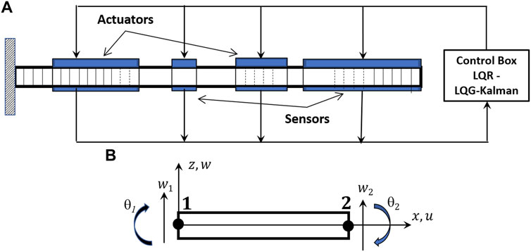
FIGURE 1. (A) Smart cantilever beam with the piezoelectric elements and controlling box. (B) Timoshenko two-nodes finite element.

2.2 Piezoelectric constitutive equations

The constitutive equations of the piezoelectric field and electromechanical behavior can be expressed by

${\sigma }_{ij}=C_{\mathit{ijkl}}{\epsilon }_{kl}-e_{\mathit{kij}}{E}_k,(7)$

$D_i=e_{\mathit{ijk}}{\epsilon }_{kl}+{ϵ}_{ik}{E}_k.(8)$

where {ɛ} and {σ} are the strain and the stress tensors, respectively, [C] is the elastic constant tensor, [e] is the piezoelectric stress coefficients, [D] is the electric displacement, [ϵ] are the electric permittivities, [E] is the electric field intensity components with E = −ϕ_,i, and ϕ is the electric potential.

2.3 Sensing equations

The output charge produced by the strain in the structure is deduced from the direct equation of piezoelectricity. The total charge Q(t) generated by the strain on the surfaces of sensors produce the total current and is given by

$i\left(t\right)=zW{e}_{31}{\int }_0^{T_P}{N}_a^T\dot{\mathbf{q}}dx(9)$

where z = t_b/2 + t_a, e₃₁ is the piezoelectric charge/stress constant, W is the width of the beam, $\dot{\mathbf{q}}$ is the time derivative of the modal coordinate vector, and $N_a^T$ is the second spatial derivative of the mode shape function of the beam. This current is converted into the open-circuit sensor voltage V^s using a signal conditioning device with gain G_c and applied to an actuator with the controller gain K_c. Therefore, the sensor output voltage can be written as

$V^s=G_{c}zW{e}_{31}{\int }_0^{T_P}{N}_a^T\dot{\mathbf{q}}dx(10)$

or as a scalar vector product

$V^s\left(t\right)={\mathbf{p}}^T\dot{\mathbf{q}}dx(11)$

where p^T is a constant vector. Assuming that the capacitance of the cable between the sensor and signal conditioning device and the temperature effects are neglected, the input voltage to the actuator V^a(t) is given by

$V^a\left(t\right)=K_c{G}_{c}zW{e}_{31}{\int }_0^{T_P}{N}_a^T\dot{\mathbf{q}}dx(12)$

Note that the sensor output depends on the derivative of the mode shape.

2.4 Actuating equations

Theoretically, the actuator strain is derived from the converse piezoelectric equation. The strain developed by the electric field E on the actuator layer is given by

${\epsilon }_A=d_{31}E=d_{31}{V}^a\left(t\right)/t_a(13)$

When the input to the actuator V^a(t) is applied in the thickness direction; the stress can be written as

${\sigma }_A=d_{31}E{V}^a\left(t\right)/t_a(14)$

The resultant moment M_A acting on the beam is determined by integrating the stress through the structure thickness as follows:

$M_A=E{d}_{31}\bar{z}{\int }_{l_p}{N}_{\theta }{V}^a\left(t\right)(15)$

where $\bar{z}$ is the distance between the neutral axis of the beam and the piezoelectric layer and ${[N_{\theta }]}^T$ is the first spatial derivative of the mode shape function of the beam.

The control force applied by the actuator can be written as

$f_{\mathit{ctrl}}=E{d}_{31}\bar{z}{V}^a\left(t\right)(16)$

Using a constant vector h^T, the force of control can be expressed in a scalar product as

$f_{\mathit{ctrl}}=\mathbf{h}{V}^a\left(t\right)(17)$

If an external force f_ext is applied, the total force vector of control becomes

$f_{\mathit{tot}}=f_{\mathit{ctrl}}+f_{\mathit{ext}}(18)$

2.5 Monte Carlo procedure description

The Monte Carlo method is used here to select randomly the number of sensors and their discrete location under some criteria. This is accomplished by minimizing the variance based on randomly chosen points representing the sensor’s location. The method is not detailed in this study. One can find some detailed formulations in Swann and Chattopadhyay (2006). These points, assigned randomly, generated measurements based on a specified distribution. First, it is necessary to define some variables such as structure dimensions, the grid division, the nodal density, and the number of repetitions in the Monte Carlo algorithm. The division map depends on the predefined dimensions of the structure. The data are randomly produced for each grid point established from the defined statistical criteria of the model. Random grid points are chosen from the grid map and the analysis is accomplished based on the respective locations of these points. The mean-variance results are calculated and stored as optimization variables. These steps are reproduced and repeated until the minimum mean variance is found. The sensor locations that generated the minimum mean variance are therefore the most optimal sensor placement based on the chosen number of repetitions.

3 Reduced order model

A two-node beam element with two mechanical (ω, θ) and one electric (ϕ) dof at each node is considered (Figure 1). The beam has been decomposed into 100 elements of 30 cm length. The finite element model of the beam is derived using Hamilton’s principle, and the compact equation of motion for undamped system with electromechanical coupling can be written as

$M_{qq}\ddot{q}+K_{qq}q+K_{q\varphi }\varphi -F=0(19)$

$K_{\varphi q}q+K_{\varphi \varphi }\varphi -Q_a=0(20)$

where K_qϕ and K_ϕϕ are the global stiffness matrix due to electromechanical coupling and the global stiffness matrix due to the electric dof, respectively; ϕ is the electric potential vector corresponding to the piezoelectric actuators; Q_a is the vector of electric charge. Using back substitution for ϕ from Eq. 20 into Eq. 19 and taking into account the damping effect, the governing second-order differential equation for the damped system in a compact form is given by

$M\ddot{X}\left(t\right)+C\dot{X}\left(t\right)+KX\left(t\right)=F\left(t\right)(21)$

where M, C, and K denote the mass, Rayleigh damping, and stiffness matrices of a full order system of size n × n, respectively. Also, X(t), same as $(q(t)),\dot{X}(t)$ and $\ddot{X}(t)$, represent the displacement, velocity, and acceleration vector of size n × 1, respectively. To apply the reduced model, Eq. 21 will be used in all next theoretical equations and numerical simulations.

The reduced process is a global reduction algorithm that is based on the eigenvalue analysis of the FEM model. There are two reduction process levels; reduction in the number of modes and reduction in dofs. The transformation matrix obtained using this algorithm transform the full model to a lower subspace using selected eigenmodes with few arbitrary dofs. With this modal matrix, a system can be written in terms of modal coordinates and for n_m eigenmodes as

$X\left(t\right)={\psi }_{\left(n\times n_m\right)}{\widehat{q}}_{\left(n_m\times 1\right)}\left(t\right)(22)$

If only n₁ eigenmodes are considered, the solution can be written as

$X\left(t\right)={\psi }_{\left(n\times n_1\right)}{q}_{\left(n_1\times 1\right)}\left(t\right)(23)$

By classifying the full order system into master and slave dofs and retaining only “n_m” eigenmodes in Eq. 23, we get in terms of active dofs

$X\left(t\right)=\left\{\begin{array}{c}\hfill X^m\left(t\right)\hfill \\ \hfill X^s\left(t\right)\hfill \end{array}\right\}\approx \left\{\begin{array}{c}\hfill {\psi }^m\left(t\right)\hfill \\ \hfill {\psi }^s\left(t\right)\hfill \end{array}\right\}.{\widehat{q}}_j\left(t\right)(24)$

where ${\widehat{q}}_{n_m}$ is the modal matrix having “n_m” modes, and superscripts m and s correspond to master and slave, respectively. Also here, ${\psi }^mϵ{\mathfrak{R}}^{m\times n_m}$ and ${\psi }^sϵ{\mathfrak{R}}^{{\left(\right.}^{\left.n-m\right)\times n_m}}$. Considering only the master dofs, the modal response can be given as

${\widehat{q}}_{n_m}\left(t\right)={\psi }_T^m{X}^m\left(t\right)(25)$

where ${\psi }_T^m$ is the generalized inverse of ψ^m. Since the matrix ${\psi }_T^m$ may not be a square, the number of modes and number of dofs in the analysis may be the same and depends on the problem and hence the matrix. We can find in the study of Lal et al. (2017) the different possible cases of the selection of modes and dofs. Substituting Eq. 25 in Eq. 24, we get

$X\left(t\right)=\psi {\psi }_T^m{X}^m\left(t\right)=T_r{X}^m(26)$

where $\psi {\psi }_T^m$ is the transformation matrix (T_r) that transforms the full system into the reduced system model. With this transformation matrix, the full order system matrices in the reduced model become

$M_r=T_r^{T}M{T}_r;K_r=T_r^{T}K{T}_r;C_r=T_r^{T}C{T}_r(27)$

Here, M_r, K_r, and C_r represent, respectively, the reduced mass, the reduced stiffness, and the reduced damping matrices. Note that the selection of modes and dofs are governed by the type of the structure and the conditions of external charges.

4 Active control implementation

4.1 Optimal and robust controls

There is a significant difference between optimal and robust control strategies. Optimal control seeks to optimize a performance index over a span of time, while robust control seeks to optimize the stability and quality, and robustness of the controller given the uncertainty in the plant model, feedback sensors, and actuator outputs. Optimal control assumes that the model is perfect and optimizes the provided data. If the model is imperfect, the controller is not necessarily optimal. It is only optimal for a provided functional and specific cost. The LQR control is only truly optimal for a completely linear plant and a quadratic cost index. Robust control assumes that the model is imperfect. For example, some parameters in the s system model are believed to be in a certain range but are not surely known. Controllers H₂, H∞, or others can be used in this case to decide which signals of control are admissible based on the level of uncertainty in basic parameters.

4.2 Active control in the reduced model

Using reduced representation, the dynamic equations of the structure are given by

$M_r{\ddot{X}}^m\left(t\right)+C_r{\dot{X}}^m\left(t\right)+K_r{X}^m\left(t\right)=F_r\left(t\right)(28)$

For MIMO systems, Eq. 28 in the state space form can be written as

${\dot{X}}^m=A^m{X}^m+B^m{u}^m(29)$

where

$A^m=\left[\begin{array}{cc}\hfill 0\hfill & \hfill I\hfill \\ \hfill -M_r^{-1}{K}_r\hfill & \hfill -M_r^{-1}{C}_r\hfill \end{array}\right],B^m=\left[\begin{array}{c}\hfill 0\hfill \\ \hfill M_r^{-1}{F}_r\hfill \end{array}\right](30)$

and X^m is (m × 1) state vector.

4.3 LQR control

The linear quadratic regulator (LQR) controller is used and implemented on the proposed reduced model as shown in Figure 2. The optimal control input to the actuator for vibration suppression is obtained through LQR, which minimizes the cost function (J) defined by

$J=\underset{\tau \to \infty }{\lim }\frac{1}{\tau }\left[{\int }_0^{\infty }\left\{{\left(X^m\right)}^{T}Q\left(X^m\right)+{\left(u^m\right)}^{T}R\left(u^m\right)\right\}dt\right](31)$

where Q and R are weighting matrices of system states X^m and the control input u^m.

FIGURE 2

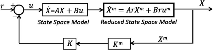
FIGURE 2. The LQR control design diagram in the reduced model.

The minimization of the quadratic cost function defined in Eq. 31, subjected to the equation of motion, gives the state feedback in form of required control input u^m given by

$u^m=-K_s{X}^m(32)$

where K_s is the (m × r) gain matrix obtained through the proposed reduced model. The closed-loop optimal gain is calculated by solving the reduced-matrix Riccati equation. With this gain matrix, the control input needed for controlling the full model dynamics of the structure is estimated. The capacitance of the sensor patch at ambient temperature Z_s can be written as

$Z_s={\breve{K}}_{\varphi \varphi }^e=\left(\left[K_{\varphi \varphi }^e\right]+\left[{\tilde{K}}_{\varphi \varphi }^e\right]\right)(33)$

where $[K_{\varphi \varphi }^e]$ is the capacitance of piezoelectric patch at reference temperature and $[{\tilde{K}}_{\varphi \varphi }^e]$ is change in the capacitance of the piezoelectric patch at a temperature other than reference temperature. For a given temperature, the voltage generated across the piezoelectric patch and the modal force are as follows:

$V={\left[K_{\varphi \varphi }^e\right]}^{-1}\left[Q_{ext}^e+\left[K_{\varphi \varphi }^e\right]\left\{u_e\right\}\right](34)$

$\left\{F_c\right\}={\left[U\right]}^T\left\{\left[K_{u\varphi }^e\right]{\left[K_{\varphi \varphi }^e\right]}^{-1}{Q}_{ext}\right\}(35)$

If the identical sensor and actuator patches function at the same temperature, the modal control force becomes

$F_c=-{\left[U\right]}^T\left[K_{u\varphi }^e\right]V_{ext}(36)$

4.4 LQG control and kalman filtering

Generally, the Kalman filter is a computational algorithm that aims to update the sequence of time and measurement in order to estimate the responses of a given system. Some works are studied using this filtering for optimal control (Simon et al., 2003) and for fuzzy discrete-time dynamic systems (Anderson and Moore, 1979). Figure 3 shows the design and the implementation of the LQG-Kalman scheme in the reduced model. The filter has been added to the LQG regulator and process and measurement noises are introduced. The state space can be represented as the following linear stochastic difference equation:

$\left\{\dot{x}\right\}=\left[A_d\right]\left\{x\right\}+\left[B_d\right]u+w_d(37)$

FIGURE 3

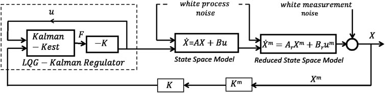
FIGURE 3. The LQG control with the Kalman filter design in the reduced model.

In order to control the response of the structure, we need to convert uncoupled equations into a state-space model. The general modal equation can be written as

$\left\{\dot{s}\right\}=\left[A\right]\left\{s\right\}+\left[B\right]V_{ext}+\left[G\right](38)$

The output of the system is a function of s and is given by

$\left\{y\right\}=\left[C\right]\left\{s\right\}(39)$

The first modal control force, the control voltage, and the sensor voltage output are, respectively, given by

${F_c}_1=-{\left[U\right]}^T\left[K_{u\varphi }^e\right]\left.\left\{V_{ext}\right\}\right),(40)$

$V_{ext}={\left({\left[U\right]}^T\left[K_{u\varphi }^e\right]\right)}^{-1}k{\dot{\eta }}_{est},(41)$

$V_{sens}={\left[K_{\varphi \varphi }^e\right]}^{-1}\left[\left[K_{u\varphi }^e\right]\left\{u_e\right\}\right].(42)$

where ${\dot{\eta }}_{\mathit{est}}$ is estimated using the Kalman observer.

Modal displacements and velocities are estimated using the Kalman observer/estimator and can be constructed as follows:

$\left\{{\dot{\eta }}_{\mathit{est}}\right\}=\left[A_d\right]\left\{{\eta }_{\mathit{est}}\right\}+\left[B_d\right]V_{\mathit{ext}}+\left[L\right]\left(V_{\mathit{sens}}-\left[X\right]\left\{{\eta }_{\mathit{est}}\right\}\right),(43)$

$\left\{{\dot{\eta }}_{\mathit{est}}\right\}=\left\{{\eta }_{\mathit{est}}\right\}+\left[M\right]\left(V_{\mathit{sens}}-\left[X\right]\left\{{\eta }_{\mathit{est}}\right\}\right).(44)$

where η_est is the estimated full state vector and [A_d] and [B_d] are discretized forms of matrices of the state equation; [L] and [M] are Kalman filter gain matrices; V_sens is the sensor voltage; and X is the sensor location vector. Matrices [B], [X], [L], and [M] and the state vector ${\dot{\eta }}_{\mathit{est}}$ all depend upon electromechanical and permittivity coefficients of the used piezoelectric material.

The external control voltage that gets applied on the piezoelectric actuator patch “i” placed on the element number “i” corresponding to the modal control force is given by (Garrido et al. ,2014)

$V_{\mathit{ctrl}}=\frac{-G_v{\dot{\eta }}_{\mathit{est}}}{{\left[U\right]}^T{f}_c{Z}_{\mathit{act}}}(45)$

where G_v is the gain of the velocity feedback controller, U is the modal matrix of the first three modes, Z_act is the capacitance of the actuator, and f_c is the vector of the electromechanical constant of the actuator.

5 Discussion

To implement the control process and to establish a comparison between the two methods of control already detailed, a smart structure is considered and shown in Figure 1. The structure consists of a cantilever Timoshenko beam modeled and multiple pairs of piezoelectric patches bonded on both sides of the beam. Piezoelectric elements are distributed symmetrically along the top and bottom of the beam covering one or more finite elements. Graphite-epoxy (T300-976) is chosen as the beam material and PZT (G1195N) as the piezoelectric material. The patches of actuators have been placed at the top side of the beam while sensors are at the bottom for high sensitivity to deformations. Geometric and material properties are given in Table 1. The beam is discretized by the finite element method in the full and reduced model with 100 elements distributed over six regions along the length. Each element has two nodes with two mechanical dofs and one electrical dof. The full model has in total of 100 FEs with 302 dofs and therefore 404 control states. Considering modal analysis and retaining just the first modes, the Monte Carlo simulation process is used to obtain statistical results to get the probabilistic description of the desired response values of the model.

TABLE 1

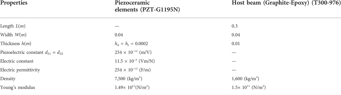
TABLE 1. Material and physical properties of piezoelectric elements and the host beam.

To establish the control comparison, a practical example of distribution based on the location of sensors is considered. To do this, different sizes and numbers of FE by sections are distributed as follows:

Section 1 with 17 elements of 1 (mm) size, section 2 with 25 elements of 3 (mm) size, section 3 with one element of 8 (mm) size, section 4 with 25 elements of 4 (mm) size, section 5 with 20 elements of 6 (mm) size and, and section 6 with 12 elements of 15 mm size.

In this example, all figures in the study are obtained with 10 distributed sensors. This gives 160 mechanical dofs and the selection is limited to 46 and 112 dofs. The dimensions of sensors by nodes are chosen as follows:

04 sensors with 04 nodes (32 dofs), 03 sensors with 08 nodes (48 dofs), 02 sensors with 12 nodes (48 dofs), 01 sensors with 16 nodes (32 dofs).

Note here that the number of dofs can be selected automatically for a given number of sensors. The number and the position of sensors can be modified easily in the software script. Therefore, the control quality can be improved by taking the few numbers of dofs (or nodes) concerning the nature of the beam mode vibration. For a higher number, the control response will not change even after adding sensors and consequently the number of selected dofs. For the first modes, the reduced modal space is established and the desired response values are determined. This allows to reduce the execution time and save computational costs.

To illustrate vibration modes, the three first mode shapes of the beam having, respectively, frequencies 7.37, 43.6, and 125.41Hz, are deduced. Figures 4 and 5 show frequency responses in Bode diagrams of uncontrolled and controlled responses corresponding to full and reduced models. Figures 6 and 7 illustrate the impulse responses of displacement in full and reduced models using the LQR control. Figure 8 shows a comparison of the impulse response in the reduced model between the two procedures of control considering 112 dofs of 10 distributed sensors. The variation of electric input of the actuators applying the LQR control is verified and shown in Figures 9–11 with selections of 46 and 112 dofs.

FIGURE 4

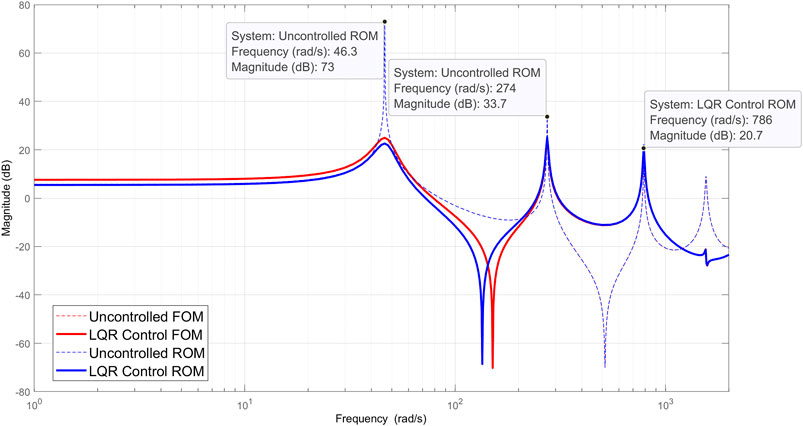
FIGURE 4. Frequencies of the three first modes in full and reduced models using the LQR control with 46 dofs of 10 distributed sensors.

FIGURE 5

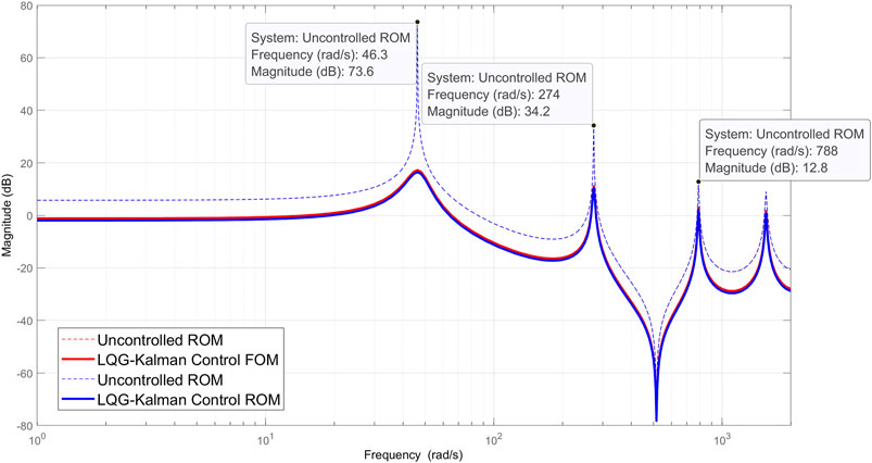
FIGURE 5. Frequencies of the three first modes in full and reduced models using the LQR control wth 112 dofs of 10 distributed sensors.

FIGURE 6

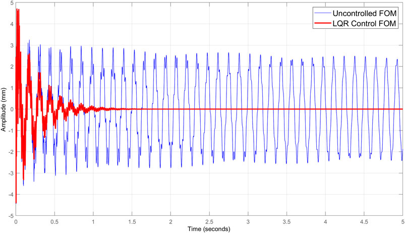
FIGURE 6. Impulse response in the full model case using LQR control and considering 112 dofs of 10 distributed sensors.

FIGURE 7

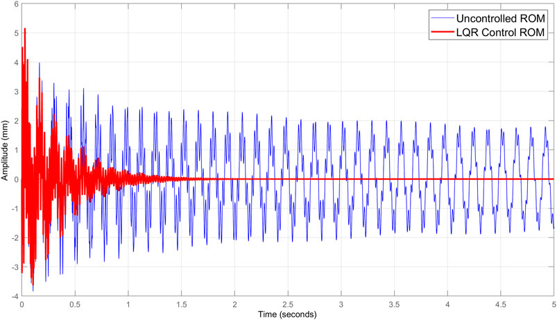
FIGURE 7. Impulse response in the reduced model case using LQR control and considering 46 dofs of 10 distributed sensors.

FIGURE 8

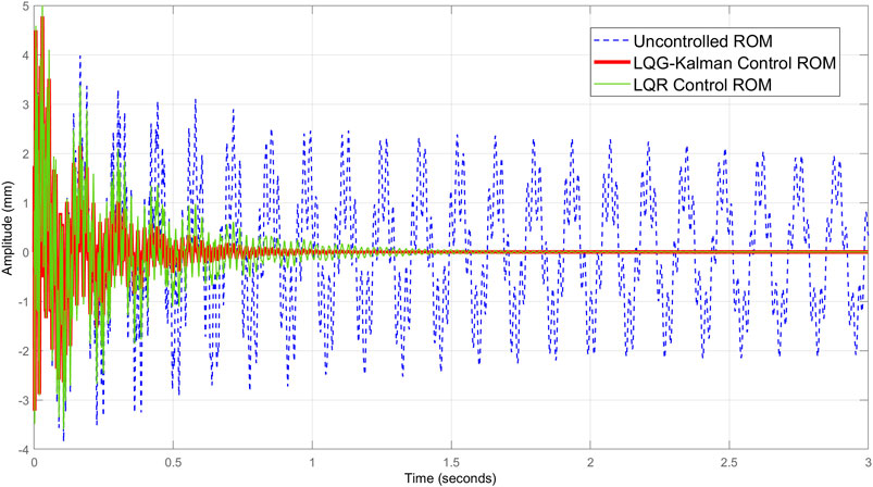
FIGURE 8. Impulse response in the reduced model case using LQR and LQG-Kalman controls with 112 dofs of 10 distributed sensors.

FIGURE 9

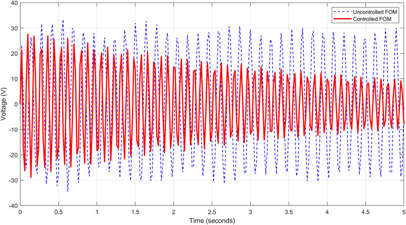
FIGURE 9. Voltage response in the full model case using LQR and considering 46 dofs of 10 distributed sensors.

FIGURE 10

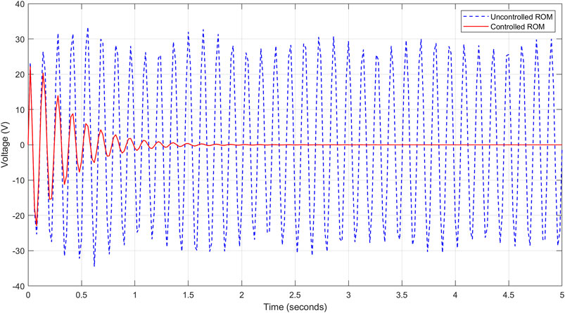
FIGURE 10. Voltage response in the reduced model case using the LQR Control and considering 46 dofs of 10 distributed sensors.

FIGURE 11

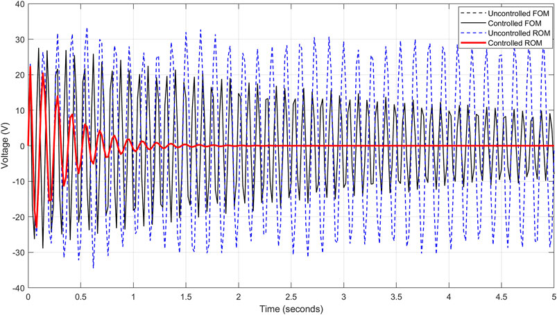
FIGURE 11. Voltage response in full and reduced models using the LQR control with 112 dofs of 10 distributed sensors.

The Monte Carlo simulation is performed to select the active dofs and dominant modes to be used in the reduced model. The selection depends on the geometry of the structure, the nature of distribution, and the values of the desired responses. Two cases of selection are retained in this application; the first with 112 dofs and the second 46 with 10 distributed sensors. The results of simulations are presented to compare the responses of control under multiple configurations. Figure 12 gives the response of the full model without control considering the selections of 46 and 112 dofs. In the full model case, Figure 13 shows the responses of the LQG-Kalman control under the same conditions as in Figure 12. Figure 14 presents a comparison in the reduced model case of LQR and LQG-Kalman controls considering only the selection of 46 dofs.

FIGURE 12

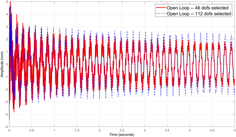
FIGURE 12. Response of the full model without control considering the selections 46 and 112 degrees of freedom.

FIGURE 13

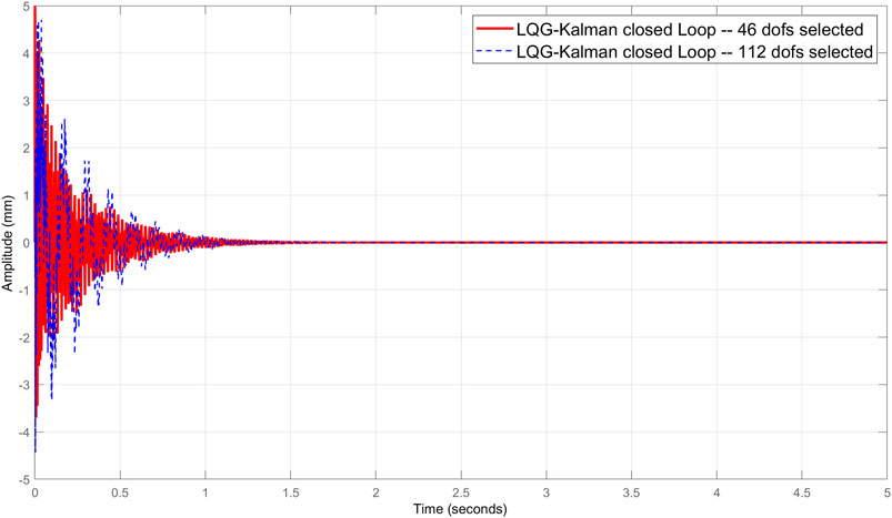
FIGURE 13. Responses of the LQG-Kalman control considering the selections of 46 and 112 degrees of freedom (the full model case).

FIGURE 14

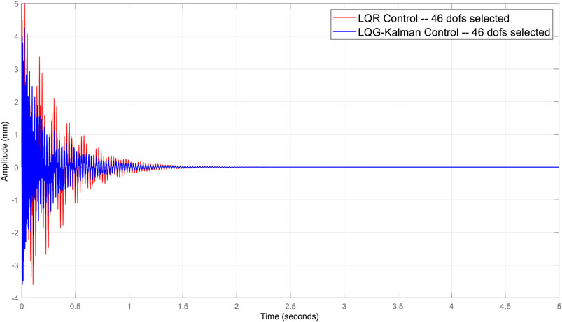
FIGURE 14. Comparison of LQR and LQG-Kalman controls considering only the selection of 46 degrees of freedom (the reduced model case).

6 Conclusion

In this study, a discretized FEM in a reduced model applied to a Timoshenko beam is formulated and presented. A control analysis based on LQR and LQG-Kalman algorithms is detailed. State spaces of the two methods of control are adapted and transformed in the reduced design. In order to optimize the number of active nodes (or their relative dofs), the Monte Carlo simulation is introduced and exploited in the control setup. An example of the distribution and selection of sensors is detailed and presented. Mode shapes, displacements, actuator inputs, and sensors outputs are simulated and plotted.

In comparison with the LQR control, it is observed that the reduced LQG-Kalman design coupled with Monte Carlo simulation gives good results for low voltages of electric actuation and a large number of selected active dofs. The reduced model is based on the eigenvalue analysis of the full model to constitute the relative transformation matrices. This analysis is a costly process and a necessary step in computation. With the present scheme, it is observed that compilation time, in the two studied cases of selected nodes, was reduced by 30–50 percent. For optimal control, the model reduction must be accompanied by an appropriate technique of selection of dofs for a significant optimization in time and cost of computation.

Data availability statement

The original contributions presented in the study are included in the article/Supplementary Material; further inquiries can be directed to the corresponding author.

Author contributions

All authors listed have made a substantial, direct, and intellectual contribution to the work and approved it for publication.

Conflict of interest

The authors declare that the research was conducted in the absence of any commercial or financial relationships that could be construed as a potential conflict of interest.

Publisher’s note

All claims expressed in this article are solely those of the authors and do not necessarily represent those of their affiliated organizations, or those of the publisher, the editors, and the reviewers. Any product that may be evaluated in this article, or claim that may be made by its manufacturer, is not guaranteed or endorsed by the publisher.

References

Amini, A., Mohammadimehr, M., and Faraji, A. (2020). Optimal placement of piezoelectric actuator/sensor patches pair in sandwich plate by improved genetic algorithm. Smart Struct. Syst. 26, 721–733. doi:10.12989/sss.2020.26.6.721

CrossRef Full Text | Google Scholar

Anderson, B., and Moore, J. (1979). Optimal filtering. New Jersey: Thomas Kailath Editor.

Google Scholar

Callahan, J., Avitabile, P., and Madden, R. (1989). “System equivalent reduction expansion process,” in Proceedings OF 7th International Modal Analysis Conference. Editors U. College, and S. for Experimental Mechanics, 29–37.

Google Scholar

Cao, X., Tanner, T., and Chronopoulos, D. (2020). Active vibration control of thin constrained composite damping plates with double piezoelectric layers. Wave Motion 92, 102423. doi:10.1016/j.wavemoti.2019.102423

CrossRef Full Text | Google Scholar

Chen, S. H., Zheng, L. A., and Chou, J. H. (2007). A mixed robust/optimal active vibration control for uncertain flexible structural systems with nonlinear actuators using genetic algorithm. J. Vib. Control 13 (2), 185–201. doi:10.1177/1077546307070228

CrossRef Full Text | Google Scholar

Garrido, H., Curadelli, O., and Ambrosini, D. (2014). A straightforward method for tuning of Lyapunov based controllers in semi active vibration control applications. J. Sound Vib. 51, 1119–1131. doi:10.1016/j.jsv.2013.10.029

CrossRef Full Text | Google Scholar

Gupta, V., Sharma, M., and Thakur, N. (2012). Active structural vibration control: Robust to temperature variations. Mech. Syst. Signal Process. 33, 16780. doi:10.1016/j.ymssp.2012.07.009

CrossRef Full Text | Google Scholar

Hsiao, F. H., Xu, S. D., Wu, S. L., and Lee, G. C. (2006). Lqg optimal control of discrete stochastic systems under parametric and noise uncertainties. J. Frankl. Inst. 343 (3), 279–294. doi:10.1016/j.jfranklin.2006.02.038

CrossRef Full Text | Google Scholar

Hsieh, W. (2002). Nonlinear principal component analysis by neural networks. Tellus A 53 (5), 599–615. doi:10.1034/j.1600-0870.2001.00251.x

CrossRef Full Text | Google Scholar

Hu, J., Zhang, X., and Kang, K. (2018). Layout design of piezoelectric patches in structural linear quadratic regulator optimal control using topology optimization. J. Intelligent Material Syst. Struct. 29, 2277–2294. doi:10.1177/1045389X18758178

CrossRef Full Text | Google Scholar

Hu, J., and Zhu, D. (2012). Vibration control of smart structure using sliding mode control with observer. J. Comput. (Taipei). 7 (2), 491–506. doi:10.4304/jcp.7.2.411-418

CrossRef Full Text | Google Scholar

Hughes, P., and Skelton, R. (1981). Modal truncation for flexible spacecraft. J. Guid. Control Dyn. 4 (3), 291–297. doi:10.2514/3.56081

CrossRef Full Text | Google Scholar

Kim, H. S., Sohn, J. W., and Choi, S. B. (2011). Vibration control of a cylindrical shell structure using macro fiber composite actuators. Mech. Based Des. Struct. Mach. 39 (4), 491–506. doi:10.1080/15397734.2011.577691

CrossRef Full Text | Google Scholar

Lal, H., Sarkar, S., and Gupta, S. (2017). Stochastic model order reduction in randomly parametered linear dynamical systems. Appl. Math. Model. 333 (4), 744–763. doi:10.1016/j.apm.2017.07.043

CrossRef Full Text | Google Scholar

Rader, A. A., Afagh, F. F., Yousefi-Koma, A., and Zimcik, D. G. (2007). Optimization of piezoelectric actuator configuration on a flexible fin for vibration control using genetic algorithms. J. Intelligent Material Syst. Struct. 18 (10), 1015–1033. doi:10.1177/1045389X06072400

CrossRef Full Text | Google Scholar

Rao, A. R. M., and Anandakumar, G. (2007). Optimal placement of sensors for structural system identification and health monitoring using a hybrid swarm intelligence technique. Smart Mat. Struct. 16 (6), 2658–2672. doi:10.1088/0964-1726/16/6/071

CrossRef Full Text | Google Scholar

Sanbi, M., Saadani, R., Sbai, K., and Rahmoune, M. (2015). Thermal effects on vibration and control of piezocomposite Kirchhoff plate modeled by finite elements method. Smart Mater. Res. 2015, 1–15. doi:10.1155/2015/748459

CrossRef Full Text | Google Scholar

Sanbi, M., Saadani, R., Sbai, K., and Rahmoune, M. (2014). Thermoelastic and pyroelectric couplings effects on dynamics and active control of smart piezolaminated beam modeled by finite element method. Smart Mater. Res. 2014, 1–10. doi:10.1155/2014/145087

CrossRef Full Text | Google Scholar

Sharma, M., Singh, S. P., and Sachdeva, B. L. (2007). Modal control of a plate using a fuzzy logic controller. Smart Mat. Struct. 16 (4), 1331–1341. doi:10.1088/0964-1726/16/4/047

CrossRef Full Text | Google Scholar

Sharma, S., Vig, R., and Kumar, N. (2016). Temperature compensation in a smart structure by application of DC bias on piezoelectric patches. J. Intell. Mat. Syst. Struct. 27 (18), 2524–2535. doi:10.1177/1045389X16633769

CrossRef Full Text | Google Scholar

Simon, D., Curadelli, O., and Ambrosini, D. (2003). Kalman filtering for fuzzy discrete time dynamic systems. Appl. Soft Comput. 3, 191–207. doi:10.1016/S1568-4946(03)00034-6

CrossRef Full Text | Google Scholar

Spier, C., Bruch, J. C., Sloss, J. M., Adali, S., and Sadek, I. S. (2009). Placement of multiple piezo patch sensors and actuators for a cantilever beam to maximize frequencies and frequency gaps. J. Vib. Control 15 (5), 643–670. doi:10.1177/1077546308094247

CrossRef Full Text | Google Scholar

Swann, C., and Chattopadhyay, A. (2006). Optimization of piezoelectric sensor location for delamination detection in composite laminates. Eng. Optim. 38, 511–528. doi:10.1080/03052150600557841

CrossRef Full Text | Google Scholar

Tanaka, N., and Sanada, T. (2007). Modal control of a rectangular plate using smart sensors and smart actuators. Smart Mat. Struct. 16 (1), 36–46. doi:10.1088/0964-1726/16/1/004

CrossRef Full Text | Google Scholar

Vladimír, K., Juraj, P., Gálik, G., and Justín, M. (2021). Piezoelectric beam finite element model and its reduction and control. Strojnícky časopis - J. Mech. Eng. 71, 87–106. doi:10.2478/scjme-2021-0008

CrossRef Full Text | Google Scholar

Wang, X., Zhou, W., Zhang, Z., Jiang, J., and Wu, Z. (2021). Theoretical and experimental investigations on modified lq terminal control scheme of piezo-actuated compliant structures in finite time. J. Sound Vib. 491, 115762–62. doi:10.1016/j.jsv.2020.115762

CrossRef Full Text | Google Scholar

Willcox, K., and Peraire, J. (2002). Balanced model reduction via the proper orthogonal decomposition. AIAA J. 40 (11), 2323–2330. doi:10.2514/2.1570

CrossRef Full Text | Google Scholar