 Massimiliano Ferronato
 Andrea Franceschini
 Matteo Frigo2
94% of researchers rate our articles as excellent or good
Learn more about the work of our research integrity team to safeguard the quality of each article we publish.
Find out more
ORIGINAL RESEARCH article
Front. Mech. Eng., 27 April 2022
Sec. Solid and Structural Mechanics
Volume 8 - 2022 | https://doi.org/10.3389/fmech.2022.837196
This article is part of the Research TopicHydromechanical Instabilities in Geomaterials: Advances in Numerical Modeling and Experimental TechniquesView all 7 articles
Linear solvers usually are the most time- and memory-demanding part of a full coupled hydromechanical simulation. The typical block structure of the linearized systems arising from a fully-implicit solution approach requires the development of specialized algorithms, ensuring both robustness and computational efficiency. In particular, the design of the preconditioner to accelerate iterative methods based on Krylov subspaces is key for the overall model effectiveness. This work introduces a unifying framework for the development of preconditioning techniques in multi-physics problems, and specifically in coupled poromechanics, with the aim to provide existing methods with a novel interpretation. Three approaches, namely explicit, implicit and reverse, are considered and compared in real-world challenging benchmarks, identifying merits and drawbacks of each strategy. The proposed framework can open the way to a systematic comparison of available preconditioning tools for coupled poromechanics and help generalize the existing methods for the introduction of additional physical processes in the simulation.
Hydromechanical processes in three-dimensional porous media are governed by the coupled equations describing the matrix deformation and the fluid flow through the void spaces. Both the mechanical and the flow phenomena can be highly non-linear, including the formation of localized structures, such as fractures and channelization. Today, sophisticated real-world hydromechanical simulations are routinely required in a broad range of applications, going from geosciences, to petroleum, geotechnical, environmental and also biomedical engineering, see for instance Ferronato et al. (2010); White and Borja (2011); Hu et al. (2013); Ouchi et al. (2015); Ma et al. (2017); Gudala and Govindarajan (2021) for some applications. A key issue for the use of such models in industrial problems is the computational efficiency, which mainly relies on the properties of the resulting discrete algebraic formulation and the related linear and non-linear solvers. In this work, we focus in particular on the linear solver, which usually is by far the most time- and memory-demanding task of the entire simulation.
Several different discretization methods are available, ranging from finite difference (Gaspar et al., 2003; Boal et al., 2012) to finite volume (Chen et al., 2011; Burger et al., 2012; Asadi et al., 2014), as well as classical and mixed finite element methods (Ferronato et al., 2010; Chen Y. et al., 2018; Lee, 2018; Monforte et al., 2018; Yuan et al., 2019; Khan and Silvester, 2021; Niu et al., 2021). Despite this large variety, from the algebraic viewpoint, and independently of the actual number of physical processes accounted for, the coupled discretization of a set of partial differential equations leads to a block-structured problem that cannot be efficiently addressed by standard black-box solvers, but requires the development of specialized strategies. In 3D large-size applications, the use of sparse direct solvers is not an option, hence iterative methods must be used. In the past 15 years, a growing attention has been reserved to the iterative solution of coupled hydromechanical problems, with many works devoted to the development and implementation of both fully-algebraic approaches and discretization-based strategies. Generally speaking, solution algorithms can be grouped into two main classes: (i) sequential-implicit methods, in which the primary variables are updated one by one, iterating between the governing equations, and (ii) fully-coupled or fully-implicit methods, which solve the global system of equations simultaneously for all the primary unknowns. Sequential-implicit methods exhibit a linear convergence, but can take advantage of using distinct codes and solvers for the single-physics models. Notable examples in hydromechanics can be found in the works by Jha and Juanes (2007); Girault et al. (2016); Almani et al. (2016); Borregales et al. (2018); Dana et al. (2018), just to mention a few significant studies. One of the main numerical issues of such approaches is the stability and convergence of the overall scheme, which might not be guaranteed in any condition. In contrast, fully-coupled approaches ensure unconditional stability with a super-linear convergence, but require the design of dedicated preconditioning operators to accelerate Krylov subspace solvers such as the Generalized Minimum Residual (GMRES, Saad and Schultz (1986)) or the Bi-Conjugate Gradient Stabilized (Van der Vorst, 1992)) algorithms. This is key for the solver robustness and efficiency and has recently attracted an increasing interest from the scientific community, with the introduction of a number of different algorithms in the last years. Just to cite a few recent examples, we mention parameter-robust and spectrally-equivalent block strategies (Lee et al., 2010; Hong and Kraus, 2018), multigrid-based methods (Gaspar and Rodrigo, 2017; Chen L. et al., 2018; Bui et al., 2020), or block preconditioners based on Schur complement approximations (Castelletto et al., 2016; Frigo et al., 2021) and mixed constrained approaches (Benzi and Wathen, 2008; Bergamaschi and Martínez, 2012; Liu et al., 2016). A specific application-based technique developed for coupled poromechanics is the so-called fixed-stress split, used as both nonlinear acceleration and linear preconditioner (Castelletto et al., 2015b; Both et al., 2017; Gaspar and Rodrigo, 2017; Both et al., 2019; Hong et al., 2020).
Despite the apparent differences among the several fully-implicit algorithms, a unifying algebraic background can be recognized. Recently, Ferronato et al. (2019) have formalized a general framework to classify block preconditioners for coupled multi-physics simulations. The application of such a framework can help identify a unique basic idea underlying different strategies and make it easier to generalize the algorithms to a multiplicity of problems, possibly including an increasing number of physical processes. In this work, we aim to review from a novel and unified perspective a set of different preconditioning algorithms for coupled poromechanics, comparing their advantages and drawbacks in real-world benchmarks. The paper is organized as follows. The unifying framework developed by Ferronato et al. (2019) is first recalled and recast from a physical perspective. Then, three different approaches developed for the solution of coupled hydromechanical problems written in a mixed form, namely an approximate-inverse (Franceschini et al., 2021), a block triangular (Castelletto et al., 2016) and relaxed factorization (Frigo et al., 2019) method, are reformulated within the same framework as different variants of the same strategy. Finally, the reviewed methods are compared in a set of real-world benchmarks. A few conclusive remarks close the presentation.
The fully-implicit simultaneous numerical simulation of different physical processes, occurring at variable time and space scales, is often a very challenging task. The discretization of coupled multi-physics problems gives rise to systems of linearized equations with an inherent block structure that reflects the nature of the underlying governing equations. Assuming that n different physical processes are simulated together, the Jacobian matrix A can be generally written as:
where:
•
•
In general,
Formally, we aim to find a decoupling operator E written in the factored form:
such that the matrix S:
has no coupling blocks, i.e., it is block diagonal with non-zero blocks
the decoupling factors can be computed by solving the set of multiple right-hand side systems (Ferronato et al., 2019):
Then, the overall system with A is decoupled with each diagonal block Si given by:
The local solution of each single-physics problem with the matrix Si provides simultaneously the set of unknowns associated to all processes.
The general algebraic framework presented above can be also interpreted from a physical viewpoint as a block-reduction procedure, where the variables associated to each process are progressively eliminated. For example, by eliminating the variables associated to the first process the matrix A becomes:
where the new blocks read:
Then, the procedure continues with the elimination of the variables associated to the second process:
and so on. At the kth step of the multi-physics reduction procedure, with k = 1, … , n − 1, Eqs. 10–12 can be easily generalized as:
with A(0) = A. Trivially, the existence conditions for Eqs. 14–16 are the same as for (7), and the final diagonal blocks
Of course, this general framework cannot be exactly applied to real-world large-size problems, because both the decoupling factors F, G, and the diagonal blocks of S are dense. However, if their computation is carried out inexactly, we can use this approach as a preconditioner to accelerate the convergence of a non-symmetric Krylov subspace method, such as GMRES (Saad and Schultz, 1986) or Bi-CGStab (Van der Vorst, 1992). Effectiveness and computational efficiency of the preconditioner basically depend on the level of approximation for each block and the selected sequence of reductions.
Coupled hydromechanical simulations are typical examples of multi-physics problems. For the sake of simplicity, in this work we focus on a three-field mixed (displacement-velocity-pressure) formulation of the classical linear poroelasticity (Biot, 1941; Coussy, 2004), but this is not restrictive since similar procedures can be extended to other formulations as well, also including multi-phase flow and fractures. In particular, the introduction of inelastic behaviors for the porous medium does not impact on the general framework proposed herein once the structural block is replaced by the tangent stiffness matrix.
Let
with:
where
Let us denote with H1(Ω) the Sobolev space of vector functions with square-integrable first derivatives, i.e., they belong to the Lebesgue space L2(Ω); and let H (div; Ω) be the Sobolev space of vector functions with square-integrable divergence. Introducing the spaces:
the weak form of the IBVP (17)–(24) reads: find
where (⋅,⋅)Ω denote the inner products of scalar functions in L2(Ω), vector functions in
A widely-used discrete version of the weak form Eqs. 30–32 is based on low-order elements, such as lowest-order continuous
Let us consider a non-overlapping partition
with
where
It is well-known that the selected spaces do not satisfy the inf-sup stability constraint in the limit of incompressible fluid and solid constituents (Sϵ → 0) and undrained conditions (either κ → 0 or Δt → 0). In order to restore the solvability conditions and avoid spurious pressure modes, we introduce in the discrete mass balance Eq. 40 the pressure-jump stabilization term (Frigo et al., 2021):
where
Let
The unknown nodal displacement components {ui,n}, edge-/face-centered Darcy’s velocity components {qj,n}, and cell-centered pressures {pk,n} at time level tn are collected in vectors
where
The final matrix A of Eq. 43 has the multi-physics block structure (1), where n = 3 physical processes are coupled together. According to the definitions given above, displacements and Darcy’s velocities are uncoupled processes. In the sequel, we discuss the development of effective solvers for the hydromechanical problem in the form Eq. 43. The focus is on the preconditioning technique used in a non-symmetric Krylov subspace method based on the general framework described in Section 2. According to the different strategies used to approximate the decoupling factors and the resulting Schur complements, we distinguish among three different approaches: the explicit, implicit and reverse methods.
Using the definitions introduced in Section 2, the decoupling operators G and F for the multi-physics problem Eq. 43 read:
where Iu, Iq, and Ip are the identity operators in
Recalling from Eqs. 38–40 that
The explicit sparse computation of the decoupling factors, say
where
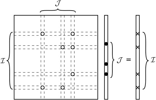
FIGURE 1. Schematic representation of the restriction applied to system (53).
In order to avoid the solution to over- or under-determined rectangular systems, we define the sets:
where
Notice that the implementation of Eq. 55 is trivially amenable for high-performance parallel computations. Then, the diagonal blocks of S can be explicitly computed as well:
The blocks Su, Sq, and Sp, which can be regarded as the result of the reduction to a sequence of SPD single-physics problems, are also inverted inexactly for the sake of preconditioning by introducing three approximations
The key factors for the quality and effectiveness of
A natural choice for
After setting the initial patterns, successive expansions are governed by an adaptive algorithm built on the one introduced by Janna and Ferronato (2011) and Janna et al. (2015b). We compute
The non-zero pattern
The exact decoupling factors Fup and Fqp are dense and their explicit computation assumes that they can be well-approximated by a sparse operator. This might not be the case in complex problems, and especially where strongly coupled conditions add to grid distortion and medium heterogeneity. This limitation can be overcome by using an implicit approximation, where Fup and Fqp of Eq. 52 do not need to be formed and their application to a vector is carried out by a matrix-by-vector product and an inexact application of either
that can be neither computed nor inverted in simple and efficient ways. This limitation can be bypassed by defining explicit physics-based approximations
The contribution
with Kb the volumetric bulk modulus. Under this hypothesis, the continuity Eq. 19 reads:
The same occurrence takes place if the deformation occurs in oedometric conditions with prevented lateral deformations, where we have (Verruijt, 1969):
with Kv the vertical uniaxial bulk modulus. Again, we have the same expression as in (61) where Kb is replaced by Kv. Therefore, the idea is to replace the mass balance Eq. 19 with:
for preconditioning purposes only, where
Introducing in (64) the discrete approximation (42) for the pressure and the basis
Following the algebraic interpretation of
The operator defined in Equation 65 was also used to obtain the so-called fixed-stress splitting scheme for the sequential solution of a finite element coupled poromechanical model (Kim et al., 2011; White et al., 2016). For this reason,
The computation of
The contribution
The final implicit preconditioning operator
where
As in any preconditioning method based on Schur complement approximations, the implicit approach requires some specific trick to define Sp in an amenable way. The main limitation of physics-based strategies, such as the one described in Section 3.2, is that they are usually very problem-dependent and do not provide the user with operative tools for improving the approximation. For example, the surrogate contributions
The idea is to properly permute the block rows and columns so as to avoid the computation of Sp. This can be done, for instance, by eliminating the pressure variables first, then Darcy’s velocities, and finally reducing to a single-physics displacement problem. For this reason, we denote this strategy as a reverse preconditioning approach. Let us first permute the matrix A as:
and eliminate the pressure variables from the second and third block rows by using the multi-physics reduction procedure described in Section 2. The matrix App, however, is SPSD, hence it cannot be safely inverted in any circumstances. To avoid such an inconvenience, we replace App in Equation 70 with αIp, where
with:
The next step should include the elimination of Darcy’s velocity from the third block row, thus implying the use of the inverse of
where
By permuting the sequence of variables back to the original displacement-velocity-pressure ordering, the resulting preconditioner reads:
and was denoted as Relaxed Physical Factorization in order to recall a similar strategy previously introduced for Navier-Stokes equations (Benzi et al., 2011, 2016).
The reverse preconditioning approach does not require the computation and the inversion of the classical Schur complement Sp, but needs inner solves, that are carried out inexactly, with
with β > 0, C a regular SPD matrix, and FFT a rank-deficient contribution. The inexact application of C(1),−1 may easily become an issue for large values of β, with a progressive deterioration of the
with C(1) defined as in (79), is carried by setting the auxiliary variable w = βFTv. System (80) then reads:
Eliminating v from the second equation we obtain:
which substituted in the first equation gives:
where βu = α−1 and βq = Δtα−1. In this way, for the application of
In order to compare the proposed algorithms and assess their numerical performances, we select four real-world test cases. They are different in terms of: (i) nature of the applications, ranging from a geotechnical problem to a deep reservoir and a regional hydrogeological model; (ii) grid type, which can be either structured or unstructured; and (iii) material properties, with a variable heterogeneous and anisotropic behavior for both the intrinsic permeability and the mechanical parameters. The test cases are as follows.
• Treporti: this model is used to reproduce the consolidation conditions of shallow heterogeneous sediments due to the presence of a trial embankment in the Venice lagoon. The surface loading/unloading process lasts 5 years, with the main purpose of characterizing the geomechanical properties of the sedimentary deposits and was developed to support the analyses for the construction of the mobile barriers located at the Venice lagoon inlets (Castelletto et al., 2015a). The porous formation consists of a sequence of alternating sandy, silty and clayey layers down to 60-m depth (Figure 2A), with a vertical intrinsic permeability and Young modulus varying in the ranges [5.1 × 10⁻¹⁶, 5.1 × 10⁻¹⁵] m2 and [2.5, 44.0] MPa, respectively. The Poisson ratio is ν = 0.15. The model represents one fourth of the embankment, thus boundary conditions are set to honour the symmetry. The only fully constrained surface is the bottom. Further details on the model can be found in Castelletto et al. (2015a).
• SPE10-16: the top 16 layers of the SPE10 Comparative Solution Project (Christie and Blunt, 2001) are used to model a compacting reservoir subject to a single-phase flow. The computational domain includes 60, ×, 220, ×, 16 hexahedral elements in the x-, y- and z-direction, respectively (Figure 2B). The reservoir is a well-known benchmark for industrial reservoir simulators, being representative of a shallow-marine Tarbert formation characterized by severe permeability and porosity variations, as shown in the figure. While the intrinsic permeability is derived from the SPE10 dataset, homogeneous mechanical properties are defined for the entire domain. In particular, we have E = 8.3 × 10³ MPa and ν = 0.3. Roller boundary conditions are imposed on all boundaries, except for the top one that is traction-free.
• SPE10-35: the model is built on top of the SPE10-16 test case by extending the simulation to the first 35 layers of the SPE10 benchmark and including the related intrinsic permeability and porosity distribution maps (Figure 2C). Mechanical properties and boundary conditions are the same as in SPE10-16.
• Chaobai: this is a regional-size hydrogeological model with the purpose of simulating land subsidence and possible ground ruptures caused by the over-exploitation of a shallow multi-aquifer system in the Chaobai River alluvial fan, North of Beijing in China. The study area has an overall extent of 1,155 km2. To account for the strongly heterogeneous nature of the sediments, a statistical inverse framework in a multi-zone transition probability approach is adopted (Zhu et al., 2016, 2020). The aquifer system is confined by an irregular bedrock located at about 550 m below the top surface (Figure 2D). More details on the model implementation and porous rock parameters are provided in Ferronato et al. (2017).
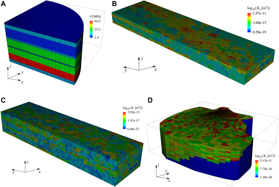
FIGURE 2. Meshes used for the numerical test cases. (A) Treporti case, showing the values of Young modulus. (B) SPE10-16, with the horizontal intrinsic permeability distribution κx = κy. (C) SPE10-35, displaying the vertical intrinsic permeability distribution κz. (D) Chaobai case, showing the vertical intrinsic permeability distribution Kz. For Chaobai, a vertical exaggeration factor of 25 is used.
For each problem, which is generally characterized by non-linear constitutive laws, we select the Jacobian matrix arising at some representative steps of a full simulation. The objective is to test the proposed linear solvers in different regimes of a hydro-mechanical problem, so as to investigate the robustness of the proposed preconditioners and in which conditions they can work best. Moreover, the selected test cases have also a different practical nature, thus involving a wide range of mechanical and hydrological parameter values. Treporti and Chaobai test cases consider shallow environments, with the former reproducing the consolidation of a soft and very low permeable layered material lying on a lagoon deposition and the latter studying the behavior of a mostly gravel aquifer with the insertion of sand and clay lenses. By distinction, the SPE10-based problems focus on a stiff and deep rock environment, where the flow dynamics typically prevails over mechanics. Table 1 summarizes the number of displacement, Darcy’s velocity and pressure DoFs, nu, nq and np, respectively, for the four test cases. Here, n and nnz represent the total number of unknowns and the global number of non-zero entries, respectively, for the Jacobian matrix of Eq. 43. It can be noticed that the models range from about 0.5 to five million unknowns.
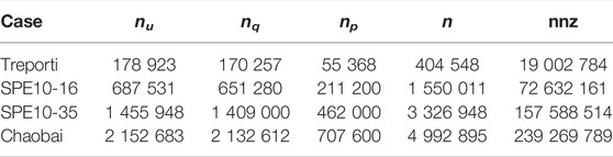
TABLE 1. Number of unknowns and matrix size for the four test cases.
A restarted GMRES (250) has been chosen as Krylov iterative method. The iterations start from the zero initial guess and are stopped when either the residual norm is reduced by eight orders of magnitude or the iteration count exceeds 1,000. In the latter case, we assume the solver fails to converge. The right-hand side is artificially generated by computing the product of A by a random vector, so that the real solution error can be also checked for consistency. The numerical results are obtained with the original (not scaled) matrix. The code is written in Fortran90 and the simulations are run using the GNU Fortran compiler (version 9.3.0). Computational performances are evaluated on a local server equipped with an Intel(R) Xeon(R) CPU E5-2643 at3.30 GHz (quadcore) and 256 GB of DIMM RAM. For all tests, a shared-memory OpenMP paradigm is used with four computing cores.
Independently of the selected explicit, implicit or reverse approach, inner preconditioners
Tables 2–5 show the numerical results obtained with the four test cases. In particular, we analyze the following parameters:
• the density μ of the preconditioner, defined as the ratio between the number of non-zero entries stored for the preconditioner and the block matrix A. This number provides a measure of the memory footprint of the preconditioner and a rough estimate of the expected application cost;
• the iteration count nit to achieve convergence. Absence of this value means that convergence was not achieved within 1,000 iterations and a failure is accounted for;
• the setup time Tsetup in seconds, accounting for the cost to compute all the terms required for the preconditioner construction. This has to be taken as the maximum setup cost needed to build the full preconditioner from scratch. Of course, in a full transient simulation even significant parts of the preconditioner can be recycled with this cost largely amortized;
• the solution time Tsol in seconds, spent by preconditioned GMRES (250) to complete the iterations;
• the total time Ttot = Tsetup + Tsol. This value has to be regarded as the maximum total time spent for the solution of a single system with the matrix A, neglecting the setup portion that can be recycled during a full transient simulation.
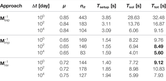
TABLE 2. Treporti test case: computational performance.
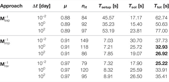
TABLE 3. SPE10-16 test case: computational performance.
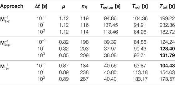
TABLE 4. SPE10-35 test case: computational performance.
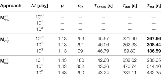
TABLE 5. Chaobai test case: computational performance. — means that convergence is not achieved within 1,000 iterations.
For each test case, three different values of the time step Δt are considered. This allows to consider the robustness and efficiency of every approach in different regimes of the hydro-mechanical problem at hand. The solver performance at each Δt value is representative of the behavior expected in three different stages of a full transient simulation. Typically, small time steps are required at the early simulation stage, so as to capture at a better detail the initial evolution, while larger and larger time steps can be safely used towards the steady state when mechanics decouples from the fluid flow. Herein we use a “small” (first line), “intermediate” (second line), and “large” (third line) time step size for each test case with respect to the characteristic consolidation time of the problem. The intermediate time step size has the order of the characteristic consolidation time, hence a time step is regarded as small or large if it is two orders of magnitude lower or higher, respectively.
In each table, bold values highlight the best performances in terms of total time. We notice that the three approaches can solve all the cases at every consolidation stage, except for the combination
Tables 2–5 show that
Finally, we observe that the selected test cases are meant to provide representative information as to the linear solver performance in different consolidation regimes, physical conditions and spatial scales, but of course they cannot cover the entire spectrum of applications. However, these different situations are expected to impact more on the parameters controlling the quality associated to the inner solvers, than on the overall decoupling effectiveness of the proposed methods.
The development of robust and efficient solvers for the linearized discrete problems arising from coupled hydromechanical applications is an important field of research. In recent years, several different algorithms for preconditioning purposes have been proposed, relying on either algebraic or physical or discretization-based considerations. In this work, we attempt to introduce a unifying framework and recast apparently different approaches within similar underlying ideas. We focus, in particular, on coupled hydromechanical problems written in a mixed form.
Based on the general algebraic framework introduced by Ferronato et al. (2019) for coupled multi-physics applications, we define a decoupling operator whose action can recast a block-structured problem into a set of independent single-physics problems. The same holds true if a standard block-reduction procedure is carried out, being only a part of the overall decoupling operator computed explicitly. According to the way such a decoupling operator is approximated, different algorithms can arise. In particular, we have investigated three approaches.
• Explicit algorithm: sparse approximations of the factors of the decoupling operator are computed explicitly with the aid of techniques borrowed from approximate-inverse preconditioners. The method is flexible and able to adapt to the different features of the problem under consideration, allowing for a straightforward computation of the Schur complement matrices. Difficulties might arise, however, when sparse approximations of the decoupling factors do not exist. In these cases, the preconditioner cost and density can increase too much, also showing a possible lack of robustness.
• Implicit algorithm: the factors of the decoupling operator are not computed explicitly, but applied to a vector by a matrix-vector product and an inexact solve with an inner single-physics block. This allows for inherently keeping a much denser, hence more effective, decoupling operator, but the resulting Schur complement matrix cannot be computed explicitly. Very effective results are obtained by introducing physics-based approximations, which typically yield efficient results in a scalable and parallel-friendly environment. However, physics-based Schur complement approximations are not flexible and do not leave control to the user.
• Reverse algorithm: the reduction sequence used in the implicit approach is reversed so as to avoid the computation of troublesome Schur complement matrices. This is carried out by replacing the pressure block with a relaxed mass matrix, where the relaxation parameter is set optimally in order to cluster the eigenspectrum of the preconditioned matrix. This approach is generally more expensive and possibly prone to near-singularity of the inner single-physics blocks, but enables the user with an important flexibility and is generally more efficient than the explicit approach.
The proposed methods can integrate each other, overall proving robust and efficient in real-world challenging applications. The present work can also open the path to a more systematic interpretation and organization of other algorithms for the linear solution to coupled hydromechanical applications, yielding to a definition of common benchmarks and a thorough comparison of algorithms.
The datasets presented in this study can be found in online repositories. The names of the repository/repositories and accession number(s) can be found below: https://gitlab.com/matteofrigo5/coupledporomechanicsmatrices.
MFe: Conceptualization, methodology, supervision, writing (Sections 1, 2, 3, 5), review and editing. AF: Software, simulations, writing-original draft (Section 4). MFr: Software, simulations, writing-original draft (Section 4).
MFr is employed by M3E Srl.
The remaining authors declare that the research was conducted in the absence of any commercial or financial relationships that could be construed as a potential conflict of interest.
All claims expressed in this article are solely those of the authors and do not necessarily represent those of their affiliated organizations, or those of the publisher, the editors and the reviewers. Any product that may be evaluated in this article, or claim that may be made by its manufacturer, is not guaranteed or endorsed by the publisher.
The Authors gratefully acknowledge Nicola Castelletto and Joshua A. White for the inspiring talks and their friendly contribution.
Almani, T., Kumar, K., Dogru, A., Singh, G., and Wheeler, M. F. (2016). Convergence Analysis of Multirate Fixed-Stress Split Iterative Schemes for Coupling Flow with Geomechanics. Comput. Methods Appl. Mech. Eng. 311, 180–207. doi:10.1016/j.cma.2016.07.036
Asadi, R., Ataie-Ashtiani, B., and Simmons, C. T. (2014). Finite Volume Coupling Strategies for the Solution of a Biot Consolidation Model. Comput. Geotechnics 55, 494–505. doi:10.1016/j.compgeo.2013.09.014
Benzi, M., Deparis, S., Grandperrin, G., and Quarteroni, A. (2016). Parameter Estimates for the Relaxed Dimensional Factorization Preconditioner and Application to Hemodynamics. Comput. Methods Appl. Mech. Eng. 300, 129–145. doi:10.1016/j.cma.2015.11.016
Benzi, M., Golub, G. H., and Liesen, J. (2005). Numerical Solution of Saddle point Problems. Acta Numerica 14, 1–137. doi:10.1017/S0962492904000212
Benzi, M., Ng, M., Niu, Q., and Wang, Z. (2011). A Relaxed Dimensional Factorization Preconditioner for the Incompressible Navier-Stokes Equations. J. Comput. Phys. 230, 6185–6202. doi:10.1016/j.jcp.2011.04.001
Benzi, M., and Wathen, A. J. (2008). “Some Preconditioning Techniques for Saddle point Problems,” in Model Order Reduction: Theory, Research Aspects and Applications (Berlin, Heidelberg: Springer), 195–211. doi:10.1007/978-3-540-78841-6_10
Bergamaschi, L., Mantica, S., and Manzini, G. (1998). A Mixed Finite Element--Finite Volume Formulation of the Black-Oil Model. SIAM J. Sci. Comput. 20, 970–997. doi:10.1137/S1064827595289303
Bergamaschi, L., and Martínez, Á. (2012). RMCP: Relaxed Mixed Constraint Preconditioners for Saddle point Linear Systems Arising in Geomechanics. Comput. Methods Appl. Mech. Eng. 221-222, 54–62. doi:10.1016/j.cma.2012.02.004
Biot, M. A. (1941). General Theory of Three‐Dimensional Consolidation. J. Appl. Phys. 12, 155–164. doi:10.1063/1.1712886
Boal, N., Gaspar, F. J., Lisbona, F. J., and Vabishchevich, P. N. (2012). Finite Difference Analysis of a Double-Porosity Consolidation Model. Numer. Methods Partial Differential Eq. 28, 138–154. doi:10.1002/num.20612
Borregales, M., Radu, F. A., Kumar, K., and Nordbotten, J. M. (2018). Robust Iterative Schemes for Non-linear Poromechanics. Comput. Geosci. 22, 1021–1038. doi:10.1007/s10596-018-9736-6
Both, J. W., Borregales, M., Nordbotten, J. M., Kumar, K., and Radu, F. A. (2017). Robust Fixed Stress Splitting for Biot's Equations in Heterogeneous media. Appl. Math. Lett. 68, 101–108. doi:10.1016/j.aml.2016.12.019
Both, J. W., Kumar, K., Nordbotten, J. M., and Radu, F. A. (2019). Anderson Accelerated Fixed-Stress Splitting Schemes for Consolidation of Unsaturated Porous media. Comput. Math. Appl. 77, 1479–1502. doi:10.1016/j.camwa.2018.07.033
Bui, Q. M., Osei-Kuffuor, D., Castelletto, N., and White, J. A. (2020). A Scalable Multigrid Reduction Framework for Multiphase Poromechanics of Heterogeneous media. SIAM J. Sci. Comput. 42, B379–B396. doi:10.1137/19m1256117
Bürger, R., Ruiz-Baier, R., and Torres, H. (2012). A Stabilized Finite Volume Element Formulation for Sedimentation-Consolidation Processes. SIAM J. Sci. Comput. 34, B265–B289. doi:10.1137/110836559
Camargo, J. T., White, J. A., and Borja, R. I. (2021). A Macroelement Stabilization for Mixed Finite Element/finite Volume Discretizations of Multiphase Poromechanics. Comput. Geosci. 25, 775–792. doi:10.1007/s10596-020-09964-3
Castelletto, N., Gambolati, G., and Teatini, P. (2015a). A Coupled MFE Poromechanical Model of a Large-Scale Load experiment at the Coastland of Venice. Comput. Geosci. 19, 17–29. doi:10.1007/s10596-014-9450-y
Castelletto, N., White, J. A., and Ferronato, M. (2016). Scalable Algorithms for Three-Field Mixed Finite Element Coupled Poromechanics. J. Comput. Phys. 327, 894–918. doi:10.1016/j/jcp.2016.09.06310.1016/j.jcp.2016.09.063
Castelletto, N., White, J. A., and Tchelepi, H. A. (2015b). Accuracy and Convergence Properties of the Fixed-Stress Iterative Solution of Two-Way Coupled Poromechanics. Int. J. Numer. Anal. Meth. Geomech. 39, 1593–1618. doi:10.1002/nag.2400
Chen, F., Drumm, E. C., and Guiochon, G. (2011). Coupled Discrete Element and Finite Volume Solution of Two Classical Soil Mechanics Problems. Comput. Geotechnics 38, 638–647. doi:10.1016/j.compgeo.2011.03.009
Chen, L., Wu, Y., Zhong, L., and Zhou, J. (2018a). Multigrid Preconditioners for Mixed Finite Element Methods of the Vector Laplacian. J. Sci. Comput. 77, 101–128. doi:10.1007/s10915-018-0697-7
Chen, Y., Chen, G., and Xie, X. (2018b). Weak Galerkin Finite Element Method for Biot's Consolidation Problem. J. Comput. Appl. Math. 330, 398–416. doi:10.1016/j.cam.2017.09.019
Christie, M. A., and Blunt, M. J. (2001). Tenth SPE Comparative Solution Project: A Comparison of Upscaling Techniques. SPE Reservoir Eval. Eng. 4, 308–317. doi:10.2118/72469-PA
Dana, S., Ganis, B., and Wheeler, M. F. (2018). A Multiscale Fixed Stress Split Iterative Scheme for Coupled Flow and Poromechanics in Deep Subsurface Reservoirs. J. Comput. Phys. 352, 1–22. doi:10.1016/j.jcp.2017.09.049
Elman, H., Silvester, D. J., and Wathen, A. J. (2014). Finite Elements and Fast Iterative Solvers: With Applications in Incompressible Fluid Dynamics. Oxford University Press.
Ferronato, M., Castelletto, N., and Gambolati, G. (2010). A Fully Coupled 3-D Mixed Finite Element Model of Biot Consolidation. J. Comput. Phys. 229, 4813–4830. doi:10.1016/j.jcp.2010.03.018
Ferronato, M., Franceschini, A., Janna, C., Castelletto, N., and Tchelepi, H. A. (2019). A General Preconditioning Framework for Coupled Multiphysics Problems with Application to Contact- and Poro-Mechanics. J. Comput. Phys. 398, 108887. doi:10.1016/j.jcp.2019.108887
Ferronato, M., Gazzola, L., Castelletto, N., Teatini, P., and Zhu, L. (2017). “A Coupled Mixed Finite Element Biot Model for Land Subsidence Prediction in the Beijing Area,” in Poromechanics VI (Reston, Virginia: American Society of Civil Engineers), 182–189. doi:10.1061/9780784480779.022
Ferronato, M., Janna, C., and Pini, G. (2014). A Generalized Block FSAI Preconditioner for Nonsymmetric Linear Systems. J. Comput. Appl. Math. 256, 230–241. doi:10.1016/j.cam.2013.07.049
Franceschini, A., Castelletto, N., and Ferronato, M. (2021). Approximate Inverse-Based Block Preconditioners in Poroelasticity. Comput. Geosci. 25, 701–714. doi:10.1007/s10596-020-09981-2
Frigo, M., Castelletto, N., and Ferronato, M. (2019). A Relaxed Physical Factorization Preconditioner for Mixed Finite Element Coupled Poromechanics. SIAM J. Sci. Comput. 41, B694–B720. doi:10.1137/18M120645X
Frigo, M., Castelletto, N., and Ferronato, M. (2022). Enhanced Relaxed Physical Factorization Preconditioner for Coupled Poromechanics. Comput. Math. Appl. 106, 27–39. doi:10.1016/j.camwa.2021.11.015
Frigo, M., Castelletto, N., Ferronato, M., and White, J. A. (2021). Efficient Solvers for Hybridized Three-Field Mixed Finite Element Coupled Poromechanics. Comput. Math. Appl. 91, 36–52. doi:10.1016/j.camwa.2020.07.010
Gaspar, F. J., Lisbona, F. J., and Vabishchevich, P. N. (2003). A Finite Difference Analysis of Biot's Consolidation Model. Appl. Numer. Math. 44, 487–506. doi:10.1016/S0168-9274(02)00190-3
Gaspar, F. J., and Rodrigo, C. (2017). On the Fixed-Stress Split Scheme as Smoother in Multigrid Methods for Coupling Flow and Geomechanics. Comput. Methods Appl. Mech. Eng. 326, 526–540. doi:10.1016/j.cma.2017.08.025
Girault, V., Kumar, K., and Wheeler, M. F. (2016). Convergence of Iterative Coupling of Geomechanics with Flow in a Fractured Poroelastic Medium. Comput. Geosci. 20, 997–1011. doi:10.1007/s10596-016-9573-4
Grote, M. J., and Huckle, T. (1997). Parallel Preconditioning with Sparse Approximate Inverses. SIAM J. Sci. Comput. 18, 838–853. doi:10.1137/S1064827594276552
Gudala, M., and Govindarajan, S. K. (2021). Numerical Investigations on Two-phase Fluid Flow in a Fractured Porous Medium Fully Coupled with Geomechanics. J. Pet. Sci. Eng. 199, 108328. doi:10.1016/j.petrol.2020.108328
Hong, Q., Kraus, J., Lymbery, M., and Wheeler, M. F. (2020). Parameter-robust Convergence Analysis of Fixed-Stress Split Iterative Method for Multiple-Permeability Poroelasticity Systems. Multiscale Model. Simul. 18, 916–941. doi:10.1137/19M1253988
Hong, Q., and Kraus, J. (2018). Parameter-robust Stability of Classical Three-Field Formulation of Biot's Consolidation Model. etna 48, 202–226. doi:10.1553/etna_vol48s202
Hu, L., Winterfeld, P. H., Fakcharoenphol, P., and Wu, Y.-S. (2013). A Novel Fully-Coupled Flow and Geomechanics Model in Enhanced Geothermal Reservoirs. J. Pet. Sci. Eng. 107, 1–11. doi:10.1016/j.petrol.2013.04.005
Janna, C., Castelletto, N., and Ferronato, M. (2015a). The Effect of Graph Partitioning Techniques on Parallel Block FSAI Preconditioning: a Computational Study. Numer. Algor 68, 813–836. doi:10.1007/s11075-014-9873-5
Janna, C., and Ferronato, M. (2011). Adaptive Pattern Research for Block FSAI Preconditioning. SIAM J. Sci. Comput. 33, 3357–3380. doi:10.1137/100810368
Janna, C., Ferronato, M., and Gambolati, G. (2010). A Block FSAI-ILU Parallel Preconditioner for Symmetric Positive Definite Linear Systems. SIAM J. Sci. Comput. 32, 2468–2484. doi:10.1137/090779760
Janna, C., Ferronato, M., Sartoretto, F., and Gambolati, G. (2015b). FSAIPACK: A Software Package for High-Perfomance Factored Sparse Approximate Inverse Preconditioning. ACM Trans. Math. Softw. 41, 1–26. doi:10.1145/2629475
Jha, B., and Juanes, R. (2007). A Locally Conservative Finite Element Framework for the Simulation of Coupled Flow and Reservoir Geomechanics. Acta Geotech. 2, 139–153. doi:10.1007/s11440-007-0033-0
Khan, A., and Silvester, D. J. (2021). Robust A Posteriori Error Estimation for Mixed Finite Element Approximation of Linear Poroelasticity. IMA J. Numer. Anal. 41, 2000–2025. doi:10.1093/imanum/draa058
Kim, J., Tchelepi, H. A. A., and Juanes, R. (2011). Stability, Accuracy, and Efficiency of Sequential Methods for Coupled Flow and Geomechanics. SPE J. 16, 249–262. doi:10.2118/119084-PA
Kolotilina, L. Y., and Yeremin, A. Y. (1993). Factorized Sparse Approximate Inverse Preconditionings I. Theory. SIAM J. Matrix Anal. Appl. 14, 45–58. doi:10.1137/0614004
Lee, J. J., Mardal, K.-A., and Winther, R. (2017). Parameter-Robust Discretization and Preconditioning of Biot's Consolidation Model. SIAM J. Sci. Comput. 39, A1–A24. doi:10.1137/15M1029473
Lee, J. J. (2018). Robust Three-Field Finite Element Methods for Biot's Consolidation Model in Poroelasticity. Bit Numer. Math. 58, 347–372. doi:10.1007/s10543-017-0688-3
Liu, H., Wang, K., and Chen, Z. (2016). A Family of Constrained Pressure Residual Preconditioners for Parallel Reservoir Simulations. Numer. Linear Algebra Appl. 23, 120–146. doi:10.1002/nla.2017
Ma, T., Rutqvist, J., Oldenburg, C. M., Liu, W., and Chen, J. (2017). Fully Coupled Two-phase Flow and Poromechanics Modeling of Coalbed Methane Recovery: Impact of Geomechanics on Production Rate. J. Nat. Gas Sci. Eng. 45, 474–486. doi:10.1016/j.jngse.2017.05.024
Monforte, L., Arroyo, M., Carbonell, J. M., and Gens, A. (2018). Coupled Effective Stress Analysis of Insertion Problems in Geotechnics with the Particle Finite Element Method. Comput. Geotechnics 101, 114–129. doi:10.1016/j.compgeo.2018.04.002
Murphy, M. F., Golub, G. H., and Wathen, A. J. (2000). A Note on Preconditioning for Indefinite Linear Systems. SIAM J. Sci. Comput. 21, 1969–1972. doi:10.1137/S1064827599355153
Nardean, S., Ferronato, M., and Abushaikha, A. S. (2021). A Novel Block Non-symmetric Preconditioner for Mixed-Hybrid Finite-Element-Based Darcy Flow Simulations. J. Comput. Phys. 442, 110513. doi:10.1016/j.jcp.2021.110513
Niu, C., Rui, H., and Hu, X. (2021). A Stabilized Hybrid Mixed Finite Element Method for Poroelasticity. Comput. Geosci. 25, 757–774. doi:10.1007/s10596-020-09972-3
Niu, C., Rui, H., and Sun, M. (2019). A Coupling of Hybrid Mixed and Continuous Galerkin Finite Element Methods for Poroelasticity. Appl. Math. Comput. 347, 767–784. doi:10.1016/j.amc.2018.11.021
Ouchi, H., Katiyar, A., York, J., Foster, J. T., and Sharma, M. M. (2015). A Fully Coupled Porous Flow and Geomechanics Model for Fluid Driven Cracks: a Peridynamics Approach. Comput. Mech. 55, 561–576. doi:10.1007/s00466-015-1123-8
Rice, J. R., and Cleary, M. P. (1976). Some Basic Stress Diffusion Solutions for Fluid-Saturated Elastic Porous media with Compressible Constituents. Rev. Geophys. 14, 227–241. doi:10.1029/rg014i002p00227
Saad, Y., and Schultz, M. H. (1986). GMRES: A Generalized Minimal Residual Algorithm for Solving Nonsymmetric Linear Systems. SIAM J. Sci. Stat. Comput. 7, 856–869. doi:10.1137/0907058
Van der Vorst, H. A. (1992). Bi-CGSTAB: A Fast and Smoothly Converging Variant of Bi-CG for the Solution of Nonsymmetric Linear Systems. SIAM J. Sci. Stat. Comput. 13, 631–644. doi:10.1137/0913035
Vassilevski, P. S. (2002). Sparse matrix element topology with application to AMG(e) and preconditioning. Numer. Linear Algebra Appl. 9, 429–444. doi:10.1002/nla.300
Verruijt, A. (1969). “Elastic Storage of Aquifers,” in Flow through Porous Media. Editor R. De Wiest (New York, NY, USA: Academic Press), 331–376.
White, J. A., and Borja, R. I. (2011). Block-preconditioned Newton-Krylov Solvers for Fully Coupled Flow and Geomechanics. Comput. Geosci. 15, 647–659. doi:10.1007/s10596-011-9233-7
White, J. A., Castelletto, N., and Tchelepi, H. A. (2016). Block-partitioned Solvers for Coupled Poromechanics: A Unified Framework. Comput. Methods Appl. Mech. Eng. 303, 55–74. doi:10.1016/j.cma.2016.01.008
Yuan, W.-H., Zhang, W., Dai, B., and Wang, Y. (2019). Application of the Particle Finite Element Method for Large Deformation Consolidation Analysis. Ec 36 (9), 3138–3163. doi:10.1108/EC-09-2018-0407
Zhu, L., Dai, Z., Gong, H., Gable, C., and Teatini, P. (2016). Statistic Inversion of Multi-Zone Transition Probability Models for Aquifer Characterization in Alluvial Fans. Stoch Environ. Res. Risk Assess. 30, 1005–1016. doi:10.1007/s00477-015-1089-2
Keywords: preconditioning, linear solver, Krylov methods, block-structured problems, coupled poromechanics
Citation: Ferronato M, Franceschini A and Frigo M (2022) On the Development of Efficient Solvers for Real-World Coupled Hydromechanical Simulations. Front. Mech. Eng 8:837196. doi: 10.3389/fmech.2022.837196
Received: 16 December 2021; Accepted: 11 March 2022;
Published: 27 April 2022.
Edited by:
Giulio Sciarra, Ecole Centrale de Nantes, FranceReviewed by:
Paolo Zunino, Politecnico di Milano, ItalyCopyright © 2022 Ferronato, Franceschini and Frigo. This is an open-access article distributed under the terms of the Creative Commons Attribution License (CC BY). The use, distribution or reproduction in other forums is permitted, provided the original author(s) and the copyright owner(s) are credited and that the original publication in this journal is cited, in accordance with accepted academic practice. No use, distribution or reproduction is permitted which does not comply with these terms.
*Correspondence: Massimiliano Ferronato, bWFzc2ltaWxpYW5vLmZlcnJvbmF0b0B1bmlwZC5pdA==
Disclaimer: All claims expressed in this article are solely those of the authors and do not necessarily represent those of their affiliated organizations, or those of the publisher, the editors and the reviewers. Any product that may be evaluated in this article or claim that may be made by its manufacturer is not guaranteed or endorsed by the publisher.
Research integrity at Frontiers
Learn more about the work of our research integrity team to safeguard the quality of each article we publish.