Intelligent Classification of Tungsten Inert Gas Welding Defects: A Transfer Learning Approach

Automated and intelligent classification of defects can improve productivity, quality, and safety of various welded components used in industries. This study presents a transfer learning approach for accurate classification of tungsten inert gas (TIG) welding defects while joining stainless steel parts. In this approach, eight pre-trained deep learning models (VGG16, VGG19, ResNet50, InceptionV3, InceptionResNetV2, Xception, MobileNetV2, and DenseNet169) were explored to classify welding images into two-class (good weld/bad weld) and multi-class (good weld/burn through/contamination/lack of fusion/lack of shielding gas/high travel speed) classifications. Moreover, four optimizers (SGD, Adam, Adagrad, and Rmsprop) were applied separately to each of the deep learning models to maximize prediction accuracies. All models were evaluated based on testing accuracy, precision, recall, F1 scores, training/validation losses, and accuracies over successive training epochs. Primary results show that the VGG19-SGD and DenseNet169-SGD architectures attained the best testing accuracies for two-class (99.69%) and multi-class (97.28%) defects classifications, respectively. For “burn through,” “contamination,” and “high travel speed” defects, most deep learning models ensured productivity over quality assurance of TIG welded joints. On the other hand, the weld quality was promoted over productivity during classification of “lack of fusion” and “lack of shielding gas” defects. Thus, transfer learning methodology can help boost productivity and quality of welded joints by accurate classification of good and bad welds.

1 Introduction

TIG welding is widely used in process industries to join many critical components/assemblies. Transfer learning-based deep learning models have the potential to enable intelligent and automated classification of welding defects for improving the quality and productivity of components joined together by welding. The following sections present an overview of machine learning and deep learning in image recognition, transfer learning and its applications in defects classification, automated identification of TIG welding defects, followed by the primary contribution aimed by the current study.

1.1 Machine Learning and Deep Learning in Image Recognition

Machine learning has been widely applied by researchers to model complex systems across varied domains such as robotics (Sekhar and Shah, 2020), lean manufacturing (Solke et al., 2022), composite machining (Sekhar et al., 2021), classification of anode effects (Zhou et al., 2018), fault diagnosis (Hu et al., 2020), machine condition monitoring (Liu et al., 2018), electric vehicles (Purohit et al., 2021), topic modeling (Shah et al., 2021b; Sharma et al., 2021), and many more. Neural networks form the core of the machine learning-based image recognition applications in vogue today (Sandler et al., 2019). Specifically, convolutional networks (ConvNets) have been widely applied in various computer vision applications (Szegedy et al., 2016), supported by high-performance computing facilities and the availability of large public image repositories such as the ImageNet (Deng et al., 2009). Convolutional neural networks were originally employed for character recognition (Le Cun et al., 1997). Their computer vision applicability became apparent by their ImageNet classification performance (Krizhevsky et al., 2012). In image recognition, the output of convolutional layers depends upon the shapes of inputs, kernel shapes, strides, and padding. ConvNets achieve high performance by preserving feature ordering, utilizing input multidimensionalities, keeping the networks sparse, and sharing same weights among different layers. ConvNets converge to a solution or arrive at a best optimal solution by successive forward and backward passes through the network. ConvNets aim at minimizing the total loss function by continuous alteration of nodal weights in the network layers over successive iterations.

The machine learning-based ConvNets were further developed to create deep convolutional networks for enhanced image detection, recognition, and classification applications (Szegedy et al., 2017). The convolutional neural networks had started with the LeNet models (LeCun et al., 1995) for feature extraction and sub-sampling tasks. These networks were further refined into AlexNets in 2012 (Krizhevsky et al., 2012). Subsequently, 2014 onward, very deep convolutional networks started being used in mainstream applications. The development of deep learning models heralded newer breakthroughs in the field of image recognition and classification (Krizhevsky et al., 2012; Sermanet et al., 2013; Zeiler and Fergus, 2014). The varied applications of these deep networks include object tracking (Wang and Yeung, 2013), object detection (Girshick et al., 2014), classification of videos (Karpathy et al., 2014), classification of human poses (Toshev and Szegedy, 2014), segmentation (Long et al., 2015), and super resolution (Dong et al., 2014). Deep learning models such as AlexNets (Krizhevsky et al., 2012) were successfully applied for all of the abovementioned applications and more. Deeper and wider network architectures such as GoogLeNet (InceptionV1) (Szegedy et al., 2015) and VGGNet (Simonyan and Zisserman, 2014) yielded higher quality classification performances across applications. The depth of deep learning models plays a critical role in attaining high-quality classification results (Simonyan and Zisserman, 2014; Szegedy et al., 2015), since the levels of feature extraction are substantiated by the network depth (number of stacked layers). In this way, deep learning models opened doors to newer classification applications wherein machine learning networks could not be applied (Erhan et al., 2014).

The prediction accuracy of deep learning networks can be improved by having large model sizes and high computational costs, provided that sufficient labeled data is available for training. However, from an efficiency point of view, lower computational costs and lower number of model parameters are desirable. Deep networks such as VGGNet (Erhan et al., 2014) have simple architecture but consume high computation power for network evaluation. Researchers have found that aggressive dimension reductions and factorizing convolutions can help generate high quality deep learning models with relatively lower computational costs (Szegedy et al., 2016). Mobile networks have also been designed to achieve effective classification accuracy even in resource-constrained mobile/embedded hardware environments (Sandler et al., 2019). Depthwise separable convolutions helped achieve classification accuracies comparable to regular convolutional layers while keeping the computation costs low. Tuning of deep neural networks has also been investigated by researchers to optimize performance and accuracy. Efforts have been made with regards to manual architecture search as well as in training algorithms to improve deep learning model designs. Specifically, researchers have explored hyper parameter optimization (Bergstra and Bengio, 2012; Snoek et al., 2012, 2015), connectivity learning (Ahmed and Torresani, 2017; Veniat and Denoyer, 2018), and network pruning methods (LeCun et al., 1990; Hassibi and Stork, 1993; Han et al., 2015, 2016; Guo et al., 2016; Li et al., 2016) to improve algorithmic architectures. Investigators have also dedicated efforts to modify connectivity maps of internal convolutional blocks (Zhang et al., 2018) and make connectivity structures more sparse (Changpinyo et al., 2017). Others (Zoph and Le, 2016; Real et al., 2017; Xie and Yuille, 2017; Zoph et al., 2018) have applied various metaheuristic algorithms (Shah et al., 2021a) including reinforcement learning and genetic algorithm to design optimum network architectures. However, some articles also (Sandler et al., 2019) reported that such optimized architectures tend to become very complex for low resource applications. In this context, transfer learning has emerged as a promising methodology of successfully applying pre-trained deep learning architectures for high accuracy classification tasks. The next subsection gives details of transfer learning and its utility in defects classification.

1.2 Transfer Learning and Its Applications in Defects Classification

Transfer learning refers to a deep learning methodology wherein the network is trained for one task involving a huge data set and is subsequently applied on a different task involving a much smaller dataset (Larsen-Freeman, 2013; Gao and Mosalam, 2018; Hussain et al., 2018). Transfer learning involves initial training of deep learning models on the features of a larger data set and subsequently applying these pre-trained models to another classification task of a smaller data set. This methodology enables transfer learning to achieve higher accuracy than the conventional approach of training deep learning models directly on the target data set from scratch (Shaha and Pawar, 2018). Transfer learning has been found to be especially suitable in cases wherein the target data set is insufficient for satisfactory training of the deep learning models (Zhu et al., 2011). Consequently, transfer learning is attracting a lot of attention with regards to image classification-based diagnostics in various applications, such as wind power prediction (Yin et al., 2021), wind turbine blade damage image classification (Yang et al., 2021), injection molding (Lockner et al., 2022), and other industrial fault diagnoses (Li et al., 2022).

Recent applications of transfer learning in welding defects classification include deep learning-based classification of welded joint quality using fully connected neural networks (FCNN) and convolutional neural networks (CNN) (Bacioiu et al., 2019). The CNN and FCNN models developed in this study achieved 89.5% and 93.4% classification accuracies respectively. In a similar study (Ajmi et al., 2020), X-ray images were used to detect weld defects in steel pipes. These images were classified using pre-trained AlexNet. They were also classified using other deep learning models (GoogLeNet, ResNet101, ResNet50, VGG19, and VGG16) without the application of any pre-training. The study showed that the pre-trained AlexNet model attained higher classification accuracy of welding defects than other deep learning architecture that were not pre-trained.

Thus, the existing deep learning methods coupled with transfer learning exhibit better classification results than direct application of deep learning models without pre-training. Furthermore, the inherent drawbacks of transfer learning can be overcome by utilizing advanced tuning methods such as progressive resizing technique (Bhatt et al., 2021). Such optimization techniques can be applied in conjunction with the transfer learning models to maximize the accuracy of weld defects classification. Accurate defects classification can yield better productivity of welded stainless steel components for various industrial/process applications.

1.3 Automated Identification of Tungsten Inert Gas Welding Defects

TIG welding was invented in the 1930s for joining aluminum and magnesium components (Weman, 2011; Jeffus, 2020). Gradually, TIG was applied to copper and steel welding and shielding applications as well (Weman, 2012). Today, TIG welding is widely used to join precision components in automotive, aerospace, and nuclear power industries among others (Bacioiu et al., 2019). TIG offers better control over welding parameters because its deposition rate is independent of heat input, making it suitable for achieving high-quality welded joints. The TIG welding process is also highly flexible, which makes it widely applicable. However, its process flexibility also renders weld pool complexities in different applications, which are effectively assessed and controlled by a high-skilled labor. Hence, a lot of research has been conducted to investigate various aspects of effective TIG welding quality assessment and control (Kovacevic et al., 1996; Lee and Na, 2002; Vasudevan et al., 2011; Liu et al., 2015; Li et al., 2018). TIG welding process monitoring includes various aspects such as metallurgy of the metals under consideration, welding image acquisition, image processing and classification to assess weld quality, and identification of welding defects. Automation of TIG quality assessment and process control is critical to ensure high production rates of welded components to meet the demands of ever growing economies. Over the past decade, researchers have explored various techniques to automate the TIG welding quality inspection process. Lucas et al. (2012) correlated the molten weld pool features with the weld depth penetration to achieve real-time measurement and control of weld uniformity. They applied laser illumination on the weld pool and video recorded the welding process for weld image acquisition. Mirapeix et al. (2007) estimated TIG welding temperature and correlated welding spectra with welding defects for manufacturing of nuclear power plant’s steam generator parts. The authors applied artificial neural networks (ANN)-based machine learning and a principal component analysis to process weld spectra data for defects identification. Song and Zhang (2007) applied one point algorithm and edge point algorithm to estimate the weld pool geometry in three dimensions, using the trajectory of the light reflected from weld pool for this purpose. Yang and Li (2015) applied ANN-based computer vision for spot weld pool geometry measurement, weld image segmentation, weld defects feature extraction, and defects classification. Günther et al. (2016) also applied machine learning for predicting weld pool features and controlling input power to the welding surface in a laser welding application. Bacioiu et al. (2019) utilized high dynamic range (HDR) cameras to monitor TIG welding of stainless steel (SS304) and applied machine learning to categorize “good” and “defective” welded joints. They applied convolutional neural networks and fully connected neural networks to identify the TIG welding defects classifications.

1.4 Primary Contribution of the Current Study

The preceding section shows that most of the researchers have employed machine learning-based automated classification of TIG welding defects in various applications. Welding defects classification accuracy can be further improved by exploring suitable deep learning model architecture. Presently, there is an open scope to investigate the application of transfer learning-based classification of TIG welding defects in stainless steel joints. The primary contribution of present study is to “transfer” suitable pre-trained deep learning models to a TIG welding image data set to achieve accurate classification of different kinds of defects. The current study utilized the TIG welding of SS304 stainless steel HDR picture data sets available online on Kaggle (Bacioiu, 2018) to further improve the welding defects classification accuracies reported in past research (Bacioiu et al., 2019).

2 Transfer Learning Methodology

As detailed in the previous sections, transfer learning refers to the training-based classification of a target data set using deep networks that have already been pre-trained on a large image data set. The transfer learning methodology adopted in the current study involved the following steps:

1. Data collection of TIG welding images.

2. Preprocessing of images.

3. Building transfer learning framework using:

a. pre-trained deep learning models as layer 0;

b. fully connected network as the subsequent layer.

4. Training the transfer learning architecture on preprocessed TIG welding images for two-class and multi-class classifications.

5. Maximizing model performances by using suitable optimizers.

2.1 Tungsten Inert Gas Welding Images Data Collection

As mentioned in the previous section, the current study utilized online data set of SS304 TIG welding HDR images uploaded by Bacioiu et al. (2019). The authors mounted an HDR camera on a robotic arm holding the torch used for welding SS304 plates of 5 and 10 mm thicknesses. The HDR camera captured high-definition pictures of the weld pool and the joint area ahead of the welding arc. SS304 grade stainless steel was chosen for the study owing to its good weldability and formability properties which make it suitable for a variety of industrial applications. The experimental layout consisted of generating a variety of welds based on the selection of optimal welding parameters (to generate good welds) and deviations from the optimal settings (to create bad welds), as shown in Table 1. Welding defects were generated due to excessive/insufficient heat inputs, travel speeds, inclusions of contaminants, and the absence of shielding inert gas supply.

TABLE 1

TABLE 1. TIG welding process parameters (* baseline settings) [(Bacioiu et al., 2019)].

The specifications of the HDR camera used for image acquisition are listed in Table 2. This camera avoided overexposure to the welding arc while maintaining sufficient exposure to the area surrounding it. Figure 1 shows sample images from the Kaggle data set corresponding to the good and five types of bad welds (Bacioiu et al., 2019). The authors collected and uploaded a total of 45,058 images from 56 welding experimental trials. The HDR camera captured 55 frames per second resulting in multiple welding images depicting different stages of every welding trial. In the current study, all welding images were distributed among training, testing, and validation data subsets for modeling deep learning models. Table 3 shows the number of welding images belonging to two-class categorization, wherein $C_0^T$ refers to the good weld (30,080 images) and $C_1^T$ represents all varieties of bad welds (14,978 images). Of the total 30,080 good weld images, 15,752 were allotted for training, 6,700 for validation, and 7,628 for testing. Similarly, the 14,978 bad weld pictures were distributed as 8,452, 2,994, and 3,532 for training, validation, and testing, respectively. Table 3 also shows the percentages of images reserved for training, validation, and testing data subsets for the two-classes $C_0^T$ and $C_1^T$. In a similar fashion, the Table 4 shows training, validation, and testing data subsets for multi-class image categories. Herein, $C_0^M$ indicates good welds, whereas $C_1^M-C_5^M$ corresponds to different welding defects viz. burn through, contamination, lack of fusion, lack of shielding gas, and high travel speeds, respectively. Table 4 also depicts the percentage of images belonging to $C_0^M-C_6^M$ allotted to the training, validation, and testing subsets for building the deep learning models.

TABLE 2

TABLE 2. Xiris XVC-1000 specifications (Bacioiu et al., 2019).

FIGURE 1

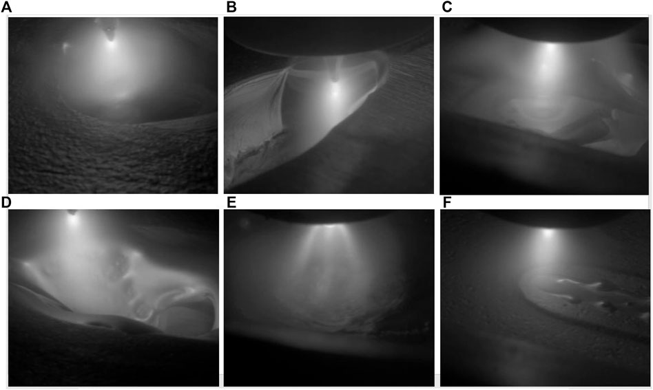
FIGURE 1. Training samples of TIG welding images. (A) Good weld, (B) burn through, (C) contamination, (D) lack of fusion, (E) lack of shielding gas, (F) high travel speed (Bacioiu, 2018).

TABLE 3

TABLE 3. Data distribution of the welding data set for two-class classification.

TABLE 4

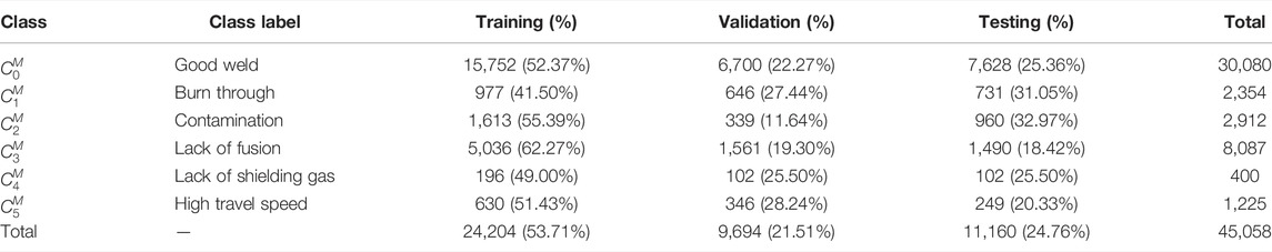
TABLE 4. Data distribution of the welding data set for multi-class classification.

2.2 Preprocessing

Preprocessing of TIG welding images was carried out through resizing, antialiasing, and normalization (Figure 2). The TIG welding defect images utilized in the current study were of size 1,280 × 700. First, all images were resized to 78 × 78 to reduce the deep learning computational time. The resized images were subsequently anti-aliased to smoothen the jagged edges in the images by using a resampling filter. The anti-aliased images were normalized to a pixel value range of 0–1 by dividing the actual number of image pixels by 255.0. The TIG welding images in the referred online data set were available in greyscale. The deep learning models trained over single channel inputs of greyscale images cannot perform as good as the models trained over three channel RGB image inputs. Hence, in the current study, a greyscale image array was replicated over the three RGB channel inputs for effective training of the transfer learning architecture.

FIGURE 2

FIGURE 2. Flowchart of transfer learning methodology for weld defects classification.

2.3 Transfer Learning With Pre-Trained Models, Optimizers, and Performance Metrics

Figure 2 depicts the process flow of the transfer learning methodology adopted in the current study. The preprocessed TIG welding images were input separately to the two-class and multi-class transfer learning architectures. Layer 0 of the transfer learning architecture contained the pre-trained deep learning models. The subsequent layers of the transfer learning architecture were formed by the first and second fully connected layers (FC1 and FC2) having 256 and 64 neurons, respectively. To avoid overfitting of the model, a dropout rate of 0.5 was considered in FC2, which was followed by the output layer yielding two-class/multi-class classifications. Table 5 depicts the feature map sizes of the eight pre-trained deep learning models considered in the current study, viz. VGG16, VGG19, ResNet50, InceptionV3, DenseNet169, Xception, Inception-ResNetV2, and MobileNetV2. These pre-trained deep learning architectures were further tuned using four optimizers: SGD, Adam, Adagrad, and Rmsprop. Thus, a total of 32 different combinations of deep learning models and optimizers were investigated for transfer learning of two-class and multi-class TIG welding defects categorizations. The performances of all deep learning models were evaluated using the metrics followed in the literature (Bacioiu et al., 2019) such as testing accuracy, precision, recall, and F1 scores. Prediction accuracy is defined as follows:

$\mathit{\text{Accuracy}}=\frac{\mathit{\text{Correct predictions}}}{\mathit{\text{Total samples}}}(1)$

TABLE 5

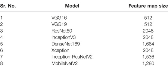
TABLE 5. Feature map sizes in pre-trained deep learning models.

The aforementioned definition of accuracy compares true positives (TP) and true negatives (TN) against true positives (TP), false positives (FP), true negatives (TN), and false negatives (FN). Model precision is a measure of prediction accuracy based on the total predicted samples, determined as follows:

$\mathit{\text{Precision}}=\frac{TP}{TP+FP}(2)$

whereas recall indicates the prediction accuracy based on the actual number of samples, given as follows:

$\mathit{\text{Recall}}=\frac{TP}{TP+FN}(3)$

High precision of bad weld classification is desirable in cases wherein the objective is to ensure that minimum good weld samples are wrongly categorized as bad. On the other hand, high recall value of bad weld classification ensures that minimum bad weld samples are incorrectly classified as good. Similarly, high precision of good weld classification ensures that minimum bad welds are incorrectly classified as good. Lastly, high recall of good weld classification implies working toward the objective that minimum good welds should be misidentified as bad. F1 scores, on the other hand, are harmonic means of recall and precision values. F1 scores give a balanced measure of both metrics by considering both false negatives as well as false positives. In this way, the F1 score is able to handle unbalanced data sets effectively. It is calculated as follows:

$\mathit{\text{F}}1\mathit{\text{Score}}=\frac{2}{\frac{1}{\mathit{\text{Precision}}}+\frac{1}{\mathit{\text{Recall}}}}=\frac{2*\mathit{\text{Precision}}*\mathit{\text{Recall}}}{\left(\mathit{\text{Precision}}+\mathit{\text{Recall}}\right)}(4)$

The performances of the four optimizers considered in the current study were determined by the evolution of training loss/accuracy as well as evolution of validation loss/accuracy over successive epochs for eight deep learning models. The relative values of training loss and validation loss profiles indicate the degree of overfitting/underfitting of the model to the training data set. If the training loss is much lesser than validation loss, it implies that the model fits the training data set much better than the validation data set. This trend indicates an overfit model that is not generalized enough to handle unseen data. On the other hand, if the training loss is much greater than the validation loss, it implies that the model fits the validation data set much better than the training data set. This trend shows that the model is underfitting the training dataset substantially. It is to be noted that validation loss is measured after each epoch, whereas training losses are determined after every batch. Therefore, convergence of validation/training losses over successive epochs and their comparable magnitudes are indicators of a well-fitted deep learning architecture.

3 Models and Optimizers

The following subsections furnish salient features of the various deep learning architectures and the optimizers considered under the scope of the current study. The suitability of various models for different applications has also been mentioned.

3.1 Overview of Pre-Trained Deep Learning Models

The following subsections give details of pre-trained deep learning models considered in the current study.

3.1.1 VGG

VGG are deep ConvNets developed by Simonyan and Zisserman (2014) in 2014. Soon, VGG models were utilized by a lot of researchers with improved performance results as compared to the conventional ConvNet architecture (Girshick et al., 2014). Researchers further explored deeper ConvNet architecture with greater convolutional layers to achieve better classification and localization accuracies. The VGG16 and VGG19 were reported as the best performing VGG deep learning models with 16 and 19 layers, respectively. These networks were successfully evaluated for large-scale image classification tasks, establishing the suitability of deep learning models for visual data classifications.

3.1.2 ResNet50

Residual networks (ResNets) were postulated by He et al. (2016) in 2016 to make deep neural network training easier. Changing the previous practice of network layers learning unreferenced functions, the authors reformulated the network layers as residual learning functions with regards to the layer inputs. Hence, ResNets learn from residual functions, and all information is always passed through layers with additional learning of newer residual functions. The authors found that the proposed residual networks achieved high accuracies at increased layer depths and were easier to optimize as well. Deep neural networks have been observed to suffer from accuracy degradation issues during convergence. The authors also addressed this issue through the formulation of deep residual learning architecture. Accuracy degradation is a limitation of solvers regarding identity mapping approximations in multiple non-linear layers. In residual learning architecture, solvers can reduce the weights of such layers to zero for identity mapping approximations. Authors claimed that identity mapping is effective against network accuracy degradation and proved to be economical as well. The authors also reported considerably higher accuracies attained by the 50-layer ResNets than their 34 layer counterparts during ImageNet classification-based evaluations.

3.1.3 InceptionV3

InceptionV1 deep learning model architecture was introduced in 2014 by Szegedy et al. (2015). In subsequent years, its improved versions were developed in the form of InceptionV2 (Howard et al., 2017) and InceptionV3 (Tieleman and Hinton, 2017). Inception models have been the best performing networks on the ImageNet data set (Russakovsky et al., 2015). An Inception model is made up of multiple Inception modules, which are convolutional feature extractors. These Inception modules are designed to work more efficiently by employing lesser number of parameters for learning data representations. Inception models decouple cross-channel and spatial correlations during convolutional mapping. The Inception architecture has been proven to consume lower computational cost than other higher performing networks (He et al., 2015). This makes it suitable for applications with constraints on computational capacity and/or memory. Specialized use of optimization can help increase the efficiency of inception networks (Psichogios and Ungar, 1994; Chen et al., 2015; Lavin and Gray, 2016). Thus, inception networks can be successfully applied in various big data scenarios (Movshovitz-Attias et al., 2015; Schroff et al., 2015). However, inception architectures tend to be complex and, therefore, are not very flexible toward modifications as per different use cases.

3.1.4 DenseNet169

DenseNet169 stands for the dense convolutional network and belongs to the family of feedforward deep learning models. These networks are deeper (with layers $>$ 100) versions of the popular convolutional neural networks typically used in image recognition machine learning modeling (Huang et al., 2017). DenseNets were designed to achieve higher performances at lesser computation expenses by reducing the number of parameters required in their model architectures. DenseNets reuse features, improve propagation of features across layers, and eliminate the issue of vanishing gradients. These deep learning models have proven to be suitable for feature extraction applications in computer vision/image recognition. Unlike ResNets (He et al., 2016), these networks combine feature maps across layers through concatenation, which makes the connectivity among their layers much denser. Each subsequent layer is fed successively larger inputs, which improves learning efficiency of the overall model. Similar concatenation approach is followed by inception networks as well (Szegedy et al., 2015, 2016); however the authors claim DenseNets to be more efficient due to their simpler architectures. DenseNets work with lesser number of parameters since their layers differentiate between the conserved and the modified information. This is unlike ResNets, which have to deal with more parameters because each layer adds its own weights while passing on the information to the next layer.

3.1.5 Xception

Xception stands for “extreme inception” since it completely decouples the mapping of spatial and cross-channel correlations in the convolutional neural network modules. The Xception network is made up of depth-wise separable convolutional layers, making it much more flexible to modify as compared to Inception models with the same number of parameters. Hence, Xception models are as easy to implement as the convolutional neural networks while retaining the efficient deep learning advantage of the inception modules.

3.1.6 Inception-ResNetV2

Szegedy et al. (2017) combined the advantages of the Inception architecture with residual connections resulting in accelerated training with high performance and low computational costs. They replaced the filter concatenations of Inception architecture with the residual connections of ResNets to enable quick training of very deep learning models while keeping computational costs low. They demonstrated the role of activation scaling to stabilize the training of very deep residual Inception networks. The authors also improved Inception architectural design by including more Inception modules and attempted further simplification of the Inception networks. The resultant Inception-ResNetV2 was reported to match the computational cost of the InceptionV4 network introduced in 2016. Inception-ResNetV2 was also reported to significantly improve image recognition performance at higher training speeds as compared to the Inception networks without residual connections.

3.1.7 MobileNetV2

The mobile networks architecture MobileNetV2 was introduced by Sandler et al. (2019). These networks were specifically designed to tackle image recognition tasks in mobile and embedded architectures with constrained computational and memory resources. Mobile network models aim computer vision accuracies at lower number of operations and memory requirements. MobileNets are composed of inverted residual layer modules with linear bottlenecks. These modules are given inputs of compressed representations having low dimensions. The compressed representations are then expanded to higher dimensions and further filtered using depth-wise convolutions. The extracted features are reverted to a low dimensional representation using a linear convolution. Linear bottleneck layers help prevent performance reduction due to the non-linear layers. This architecture is well suited for low memory constraints of mobile designs having embedded hardware with small cache memory. MobileNetV2 is an extended version of MobileNetV1 that improves detection and classification accuracy while retaining the simplicity of the first version. MobileNetV1 achieves optimal balance between accuracy and computation by employing multiplier parameters to reduce the dimensionality of layers. MobileNetV1 and MobileNetV2 were successfully evaluated by researchers for ImageNet classification, object detection, and mobile semantic segmentation applications (Sandler et al., 2019).

3.2 Overview of Optimizers

This subsection briefly discusses the various optimizers used to maximize the deep learning model performances in the current study.

3.2.1 SGD

SGD is an acronym for stochastic gradient descent optimizer that was developed to minimize computational computation complexities and enable learning per iteration while handling large data sets (Robbins and Monro, 1951). SGD requires minimal time to update gradients over successive iterations since it employs a single random sample for this purpose instead of considering all samples of a large data set. Its loss function is formulated as follows (Sun et al., 2019):

$L\left(\theta \right)=\frac{1}{N}\sum _{i=1}^N\frac{1}{2}{\left(y^i-f_{\theta }\left(x_i\right)\right)}^2(5)$

The loss function L^*(θ) for a random sample i is expressed as follows:

$L^{*}\left(\theta \right)=\frac{1}{2}{\left(y^i-f_{\theta }\left(x_i\right)\right)}^2(6)$

The gradient update based on L^*(θ) is as follows:

${\theta }^{\prime }=\theta +\eta {\left(y^i-f_{\theta }\left(x_i\right)\right)}^2{x}^i(7)$

where xⁱ is independent variable with xⁱ = $(x_1^i,x_2^i,\dots ,x_D^i)$ for i = 1, … , N, yⁱ is the target output; N is the number of training samples; and D is the total number of input features.

3.2.2 Adam

The adaptive moment estimation (Adam) is an optimization algorithm used in neural networks for computing optimal solutions (Kingma and Jimmy, 2014). Adam utilizes the learning rate (g_t) and exponential decay rates (β₁ and β₂) to determine step sizes for convergence during back propagation. The following steps are executed by the Adam optimizer:

Calculate exponential decay average of past gradients:

$m_t={\beta }_1\cdot m_{t-1}+\left(1-{\beta }_1\right)\cdot g_t(8)$

Calculate exponential decay average of past squared gradients:

$v_t={\beta }_2\cdot v_{t-1}+\left(1-{\beta }_2\right)\cdot g_t^2(9)$

Compute bias corrected first moment estimate:

$\widehat{m_t}=\frac{m_t}{1-{\beta }_1^t}(10)$

Compute bias corrected second moment estimate:

$\widehat{v_t}=\frac{v_t}{1-{\beta }_2^t}(11)$

Update weights:

${\theta }_t={\theta }_{t-1}-\eta \cdot \frac{\widehat{m_t}}{\sqrt{\widehat{v_t}+\epsilon }}(12)$

3.2.3 Adagrad

The Adagrad optimizer dynamically adjusts parametric learning rates as per the historical gradients of the previous iterations. Adagrad improves upon the SGD optimizer by “adapting” the learning rates through parameter updates during each iteration automatically, as follows:

$g_t=\frac{\partial L\left({\theta }_t\right)}{\partial \theta }(13)$

$v_t=\sqrt{\sum _{i=1}^t{\left(g_i\right)}^2+\epsilon }(14)$

${\theta }_{t+1}={\theta }_t-\eta \frac{g_t}{V_t}(15)$

where g_t is the parameter gradient θ at iteration t; V_t is the combined historical gradient of parameter θ at iteration t; and θ_t is the value of parameter θ at iteration t.

3.2.4 Rmsprop

Rmsprop or the root mean squared propagation was developed to overcome the limitation of Adagrad’s learning rate reducing to zero due to the gradients accumulated over successive iterations. Rmsprop achieves this by dividing the gradients by the square root of moving average of preceding gradients’ squares as follows:

$V_t=\sqrt{\beta V_{t-1}+\left(1-\beta \right){\left(g_t\right)}^2}(16)$

where β is the exponential decay parameter.

4 Experimental Results and Discussions

The current study involved TIG welding defects classification using transfer learning methodology. Pre-trained deep learning models were employed to obtain two-class and multi-class classifications of welding images. The model training time is expressed in terms of epochs which indicate successive iterations of layer weight alterations in the deep networks. The current study includes eight deep learning architectures with four optimizers each, totaling 32 model–optimizer combinations for each of the two-class and multi-class classification problems. Thus, considering both classifications, a total of 64 model–optimizer architectures were explored in the present study.

4.1 Performance Evaluation for Two-Class Classification

The following subsections discuss the performance evaluation results for two-class TIG welding defects classification.

4.1.1 Based on Testing Accuracies

Table 6 shows the testing accuracy results of the 32 model–optimizer architectures for two-class welded joints classifications. It is evident that the VGG19 deep learning models with SGD optimizer attained the best two-class testing accuracy of 99.69%. It is closely seconded by the VGG19 with Rmsprop optimizer architecture with 99.67% testing accuracy. Furthermore, the VGG with the Adam optimizer attained the third best testing accuracy of 99.47%. Thus, VGG19 model outperformed all other explored deep learning models in the context of two-class TIG welding defects classification. It is noteworthy that the ResNet50 with the Rmsprop optimizer attained the fourth best accuracy of 99.24%. The Xception model scored relatively lower values of testing accuracies among all explored models. The InceptionV3 model also did not perform very well relative to others. From the optimizer point of view, SGD outperformed all other optimizers for VGG16, VGG19, InceptionV3, DenseNet169, and Inception-ResNetV2. Adam attained highest testing accuracy among all optimizers for Xception and MobileNetV2, whereas Rmsprop attained highest testing accuracy among all optimizers for the ResNet50 model. Most of the model–optimizer architectures explored in the current study attained better testing accuracies than those obtained by the fully connected (89.5%) and convolutional (75.5%) neural networks applied on the same TIG welding image data by Bacioiu et al. (2019). Figure 3 depicts the two-class accuracies of all model–optimizer architectures pictorially.

TABLE 6

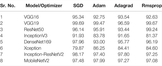
TABLE 6. Performance evaluation based on testing accuracies for two-class classification [Accuracy (%)].

FIGURE 3

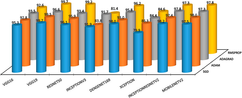
FIGURE 3. Testing accuracies for two-class classification.

4.1.2 Based on Precision, Recall, and F1 Scores

Table 7 shows two-class results of precision, recall, and F1 scores. Herein, $C_0^T$ and $C_1^T$ represent good and bad welds, respectively. The VGG19-SGD and VGG19-Rmsprop models obtained the maximum precision values of 1.00 for both the classes, which indicates perfect predictability of these models to distinguish between good and bad welds. The recall values of these two models are also near perfect—0.99 for $C_0^T$ (good welds) and 1.00 for $C_1^T$ (bad welds)—which confirms the suitability of these models to perfectly identify bad welds and almost perfect in identifying the actual good quality welded joints. Consequently, the F1 scores of these two models are also near perfect. The precision and recall values of VGG19-Adam and ResNet50-Rmsprop are slightly inferior to the VGG19-SGD and VGG19-Rmsprop models. On the other hand, models like InceptionV3-Rmsprop, InceptionV3-Adam, Xception-Rmsprop, and Xception-Adagrad attained relatively low values of precision, recall, and F1 scores. Hence, it is evident that the Inception and Xception models are unable to classify TIG welding defects as perfectly as the other explored architectures. The precision, recall, and F1 scores attained by the deep learning models in the current study are superior to those attained by the fully connected and convolution neural network architectures designed in Bacioiu et al. (2019) (on the same data set). Bacioiu et al. (2019) attained the best precision, recall, and F1 scores at 0.83, 0.99, and 0.91 $(C_0^T)$ and 0.99, 0.78, and 0.87 $(C_1^T)$. Hence, it is proved that deep learning models curated by suitable optimizers can provide much better prediction performances over conventional machine learning models.

TABLE 7

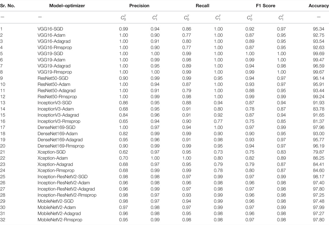
TABLE 7. Performance evaluation based on precision, recall, and F1 scores for two-class classification [Accuracy (%)].

4.2 Performance Evaluation for Multi-Class Classification

The following subsections discuss the performance evaluation results for multi-class TIG welding classifications.

4.2.1 Based on Testing Accuracies

Table 8 shows the testing accuracy results of the model–optimizer architectures for multi-class TIG welding defect classifications. The multi-class testing accuracies are inferior to two-class models, highlighting the relative difficulty in obtaining highly accurate multi-class classifications. The highest testing accuracy (97.28%) for multi-class was attained by DenseNet169 with the SGD optimizer. It was closely followed at (97.15%) by the DenseNet169 model with the Rmsprop optimizer. The VGG19 with the Adam optimizer arrived a close third with (97.12%) accuracy. Among all models, DenseNet169 attained highest testing accuracy. The Xception model once again performed poorly relative all other models. The InceptionV3 model also performed moderately in case of two-class results. Among optimizers, Rmsprop maximized testing accuracies among all other optimizers for ResNet50, Xception, Inception-ResNetV2, and MobileNetV2 models. The Adam optimizer peaked testing accuracies for VGG16 and VGG19 models, whereas the SGD optimizer helped InceptionV3 and DenseNet169 to attain best testing accuracies. Most architectures explored in the current study attained better testing accuracies than those of fully connected (69%) and convolutional (93.4%) networks designed in the previous study (Bacioiu et al., 2019). Figure 4 depicts the multi-class accuracies of all model–optimizer architectures pictorially.

TABLE 8

TABLE 8. Performance evaluation based on testing accuracies for multi-class classification [Accuracy (%)].

FIGURE 4

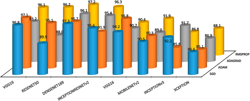
FIGURE 4. Testing accuracies for multi-class classification.

4.2.2 Based on Precision, Recall, and F1 Scores

Table 9 depicts multi-class precision, recall, and F1 scores for all 32 model–optimizer architectures. Herein, the DenseNet169-SGD architecture attained the best precision, recall, and F1 scores for all the six classes of TIG welding defects among all other models. This model performed a bit lower only in case of $C_2^M$ and $C_5^M$ recall values −0.82 and 0.79, respectively. Overall, this model attained a remarkable result, considering that many other models were unable to attain appreciable precision, recall, and F1 scores evenly across all classes. For instance, most of the deep learning models were unable to perform satisfactorily especially in case of precision values of $C_4^M$ welding defect. It may be noted that there were very few $C_4^M$ sample images available for deep learning models training as compared to other defects classes’ data sets (Table 4). There are some shortfalls in precision values for $C_3^M$ welding defect as well. Similar deficiencies are evident in case of $C_1^M$ and $C_2^M$ recall values. Some shortfalls may be observed in case of $C_5^M$ recall values as well. It is interesting to note that generally most of the models performed better in precision values as compared to the recall values for $C_1^M$, $C_2^M$, and $C_5^M$. This observation implies that deep learning models predicted lesser false positives than false negatives for these welding defects viz. burn through, contamination, and high travel speed. More false negatives mean that deep learning models are misidentifying such welding defects as good welds. On the other hand, lesser false positives imply that the models are not misidentifying good welds as the abovementioned welding defects. From a quality assurance point of view, misidentification of defective welds as good welds is an issue. On the other hand, misidentification of good welds as bad leads to loss of productivity. Hence, as regards the defects of burn through, contamination, and high travel speed, most deep learning models performed better at productivity as compared to conformance to quality.

TABLE 9

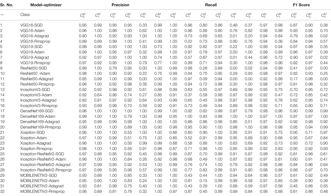
TABLE 9. | Performance evaluation based on precision, recall, and F1 scores for multi-class classification [Accuracy (%)].

In a similar fashion, the $C_3^M$ and $C_4^M$ recall values were generally observed to be superior to the corresponding precision metrics. This observation implies that the models predicted more false positives as compared to false negatives with regards to $C_3^M$ and $C_4^M$ TIG welding defects. These defect classes correspond to the lack of fusion and lack of shielding gas. More false positives over false negatives imply that the deep learning models predicted more good welds as bad and predicted lesser bad welds as good. Hence, with regards to the defects of lack of fusion and lack of shielding gas, the deep learning models predictions promoted better quality assurance at the cost of productivity losses. In a parallel observation, all models attained excellent precision as well as recall values in case of $C_1^M$, that is, good welds, which is a very encouraging result. This observation implies that all explored deep learning models architectures made no mistakes of misclassifying good welds. This result may be attributed to the fact that $C_1^M$ furnished maximum number of images in the training, validation, and testing datasets (Table 4), enabling better learning for the deep learning models. Hence, the performance of DenseNet169-SGD is appreciable considering that this model architecture successfully attained excellent precision, recall, and F1 scores across all TIG welding defects classes, despite unbalanced number of images available for training across classes.

The Xception models fared poorly in $C_3^M$ precision and $C_1^M$ recall metrics. This implies that Xception models predicted more false positives for $C_3^M$ and more false negatives for $C_1^M$ TIG welding defects. This may be further understood as misclassification of more good welds as $C_3^M$ defect, viz. lack of fusion, and greater misclassification of $C_1^M$ defect, viz. ‘”burn through” as good welds. Thus, the Xception model predictions lead to greater loss of productivity as well as lower quality assurance in TIG welding-based manufacturing. Similarly, the InceptionResNet and MobileNetV2 models performed poorly for $C_4^M$ precision. These models mostly misidentified good welds as $C_4^M$ defect, viz. lack of shielding gas, thus impacting TIG welding productivity adversely. The InceptionV3 models, on the other hand, suffered from unbalanced precision and recall accuracies across TIG welding defects classes. Interestingly, the ResNet50 models fared poorly only in case of precision and recall values for $C_4^M$ defects (lack of shielding gas). For this particular defect, the ResNet50 models totally misidentified good welds as bad and bad welds as good. With regards to the VGG models, all VGG16 models performed reasonably well across all classes, with a few exceptions in cases of $C_4^M$ precision and recall values. The VGG19 models generally performed better than the VGG16 models.

4.3 Analysis of Optimizer Performances Across Models

The previous section has already given out some details of the role of optimizers in maximizing the classification accuracies of deep learning models. In the current section, optimizer performances have been evaluated from the point of view of training loss, training accuracy, validation loss, and validation accuracy evolutions over successive training epochs.

4.3.1 Based on Two-Class Classification

Supplementary Figures S1–S4 show the two-class welding defect classification training and validation evolution graphs of all models for SGD, Adam, Adagrad, and Rmsprop optimizers, respectively. Supplementary Figure S1 training loss graph depicts that the SGD optimizer quickly reduced training loss for all models except for VGG16, VGG19, and ResNet50, wherein the training losses reduce gradually over successive epochs. Supplementary Figure S1 also shows that the deep learning models attained a little lower validation loss values as compared to their training losses (except for ResNet50). This comparison indicates that the SGD-optimized deep learning models for two-class problem are a little overfitted on the training data. Since a little data overfitting is allowed in network training, VGG19-SGD architecture attained the best two-class testing accuracy. Supplementary Figure S2 shows a similar set of graphs for the Adam-optimized deep learning models. Herein, the differences among the training and validation losses were a bit greater than those in case of the SGD-optimized models. Hence, the testing accuracies of the Adam-optimized models were a little lesser than the SGD-optimized models (Table 7). Supplementary Figure S3 depicts the Adagrad-optimized deep learning models’ training/validation loss curves. This graph also indicates little overfit models on the training data, so the Adagrad-optimized models also attained satisfactory testing accuracies. Supplementary Figure S4 shows loss curves for the Rmsprop optimizer across all deep learning models. These models also obtained decent testing accuracies owing to little differences among the training and validation losses (except for the InceptionV3 and Xception models).

Supplementary Figures S5–S8 show the training and validation accuracy curves of all deep learning models for the four optimizers considered in the current study over successive epochs. In all cases, excellent training accuracies were achieved within 20 epochs. On the other hand, almost perfect validation accuracies were attained by the models optimized with SGD, Adam, and Rmsprop. The Adagrad-optimized models attained lower validation accuracies, leading to lower testing accuracies in VGG19, ResNet50, Xception, and MobileNetV2 models (Table 7).

4.3.2 Based on Multi-Class Classification

Supplementary Figures S9–S12 show the multi-class training/validation loss curves for all deep learning models. Supplementary Figure S9 shows higher validation losses for all SGD-optimized models as compared to their training losses. This indicates that the multi-class SGD models are also a little overfitted on training data as in case of the two-class SGD-optimized architectures. Hence, the DenseNet169-SGD obtained the best testing accuracy (Table 9). Supplementary Figure S10 shows that most of the Adam-optimized models were a little more overfitted on the training datasets as compared to SGD. However, models like InceptionV2 and Xception were much more overfitted with validation losses as compared to their training losses. Models like VGG16 and VGG19 attained low validation losses, resulting in impressive testing accuracies (Table 9). Supplementary Figure S11 shows the Adagrad-optimized multi-class deep learning models validation/training losses. This figure shows relatively lower differences between the validation and the training losses, yielding better-fitted deep learning models leading to decent testing accuracies of most models except for ResNet50 (Table 9). Supplementary Figure S12 depicts a wider range of validation losses for the Rmsprop-supported architectures—Xception on the higher extreme and ResNet50 on the lowermost margin. Hence, Rmsprop maximized testing accuracies for models like ResNet50 (Table 9).

Supplementary Figures S13–S16 depict the validation/training accuracies for all deep learning models supported by the four optimizers. Except for Adagrad, all optimizers enabled the models to achieve maximum training accuracies very quickly. All optimizers helped most of the deep learning models attain validation accuracies in the range of 0.7–0.9.

4.4 Analysis of Optimizer Performances Within Models

This section deals with the training and validation losses/accuracies of the deep learning models considered in the current study, comparing the relative effects of different optimizers within each model.

4.4.1 Based on Two-Class Classification

Supplementary Figures S17, S18 showcase similar loss curves for the VGG16 and VGG19 models, with relatively lower amplitudes of validation loss curves of VGG19 than those of VGG16. The validation/training loss curves of InceptionV3 (Supplementary Figure S20), Xception (Supplementary Figure S22), and Inception-ResNetV2 (Supplementary Figure S23) models are also similar, depicting non-convergence under Rmsprop and Adam optimizers. The ResNet50 and DenseNet169 models attained comparable validation and training losses (Supplementary Figures S19, S21). Supplementary Figure S24 depicts low validation losses for MobileNetV2 with all optimizers except Rmsprop.

Supplementary Figures S25–S32 showcase the validation and training accuracies attained by the deep learning models with the help of the four optimizers. The Adam and Rmsprop optimizers helped all models (except for ResNet50) reach perfect training accuracy very quickly as compared to the SGD and Adagrad optimizers. In case of ResNet50, the Adam optimizer attained topmost training accuracy followed by Rmsprop, Adagrad, and SGD. None of the optimizers were able to help ResNet50 attain perfect training accuracy for two-class classification. In consonance with the training and validation loss values, all deep learning models recorded slightly lesser validation accuracies as compared to testing accuracies, implying little overfitting of all models. The VGG19 (Supplementary Figure S26) models attained slightly better validation accuracy than VGG16 (Supplementary Figure S25). The Adam and Rmsprop models of DenseNet169 (Supplementary Figure S29), all models of Xception (Supplementary Figure S30), and all models of Inception-ResNetV2 (Supplementary Figure S31) models attained validation accuracies greater than 0.95. The Adam and Rmsprop optimized models of InceptionV3 (Supplementary Figure S28) and MobileNetV2 (Supplementary Figure S32) did not seem to converge as good as the SGD- and Adagrad-optimized models of the same architectures.

4.4.2 Based on Multi-Class Classification

Supplementary Figures S33–S40 showcase the multi-class training and validation loss curves for all model–optimizer architectures, grouped model-wise in separate figures. The SGD and Adagrad optimizers helped all models (except ResNet50) attain lower validation losses as compared to Adam and Rmsprop optimizers. On the other hand, Adam and Rmsprop optimzers helped reduce training losses of all models in much lesser number of epochs as compared to SGD and Adagrad. Except for the VGG16 (Supplementary Figure S33), VGG19 (Supplementary Figure S34), and ResNet50 (Supplementary Figure S35) models, all other models consumed very less epochs to reduce and converge training losses to near zero values.

Supplementary Figures S41–S48 depict the multi-class training and validation accuracy graphs for all model–optimizer architectures grouped model-wise under separate plots. It is evident that the Adam and Rmsprop optimizers enabled all models (except for ResNet50) to attain maximum training accuracies in very less epochs as compared to the SGD and Adagrad optimizers. In case of ResNet50 (Supplementary Figure S43), Adam and Rmsprop attained much higher training accuracies over SGD and Adagrad. In fact, Adam and Rmsprop enabled all models (except for InceptionV3) attain better validation accuracies as well. This scenario was inverted in case of InceptionV3 (Supplementary Figure S44). In general, all VGG19 (Supplementary Figure S42) models attained better validation accuracies over the VGG16 (Supplementary Figure S41) multi-class models. The DenseNet169 Adam and Rmsprop models (Supplementary Figure S43) attained highest validation accuracies among all model–optimizer architectures, translating into correspondingly high testing accuracies as well.

5 Conclusion

The current study was based on the TIG welding image data set generated by Bacioiu et al. (2019) in which the authors collected good and defective weld images using an HDR camera. They applied fully connected and convolutional neural network-based machine learning architectures to classify the images into six categories of weldments. The same data set was utilized in the present study to improve the TIG welding defects classification accuracy by employing deep learning architectures. A total of eight different pre-trained deep learning models, namely, VGG16, VGG19, ResNet50, InceptionV3, Xception, DenseNet169, Inception-ResNetV2, and MobileNetV2 were applied via transfer learning methodology. Furthermore, each of these deep learning models were tuned by four different optimizers for maximizing classification accuracy: Adam, Adagrad, Rmsprop, and SGD, resulting in 32 varieties of model–optimizer combinations. All these models were applied for two-class (good and bad welds) and multi-class (good welds and five kinds of bad welds) classification tasks. Thus, a total of 64 model–optimizer architectures were trained—32 each for two-class and multi-class classifications. All trained and optimized pre-trained deep learning models were tested for their two-class and multi-class performances based on testing accuracy percentages, precision, recall, and F1 scores. Moreover, the evolution of models’ training/validation losses and accuracies over successive epochs were analyzed from two perspectives: the effects of individual optimizers across different models and the effects of different optimizers within individual models. The primary findings of the present study are listed as follows:

1. VGG19-SGD attained the best two-class testing accuracy (99.69%) and perfect precision, recall, and F1 scores in both TIG welding classes (good and bad welds).

2. InceptionV3 and Xception models attained relatively lower two-class and multi-class testing accuracies.

3. SGD optimizer performed better than other optimizers for most models in two-class classification.

4. DenseNet169-SGD attained the highest multi-class testing accuracy (97.28%) and excellent precision, recall, and F1 scores across all six TIG welding defects classes.

5. Rmsprop optimizer performed better than other optimizers for most models in multi-class classification.

6. Testing accuracy, precision, recall, and F1 scores of deep learning models in two-class classifications was generally superior to that in multi-class classifications.

7. Regarding the welding defects of “burn through,” “contamination,” and “high travel speed,” most deep learning models predictions favored productivity as compared to quality assurance of TIG welded joints.

8. With regards to the defects of “lack of fusion” and “lack of shielding gas,” the deep learning models predictions promoted better quality assurance at the cost of productivity losses in TIG welding-based manufacturing.

9. All explored pre-trained deep learning models architectures made no mistake of misclassifying good welds.

10. The training and validation loss evolutions over successive epochs showed that the pre-trained deep learning models were slightly overfitted on the training data set.

11. The Xception model predictions lead to greater loss of productivity and quality assurance in TIG welding-based manufacturing.

12. The InceptionResNet and MobileNetV2 model predictions mostly misidentified good welds as the welding defect of “lack of shielding gas”.

13. The ResNet50 models completely misidentified the “lack of shielding gas” welding defects as good welds and vice versa.

14. The pre-trained deep learning models architectures of the current study performed better than the machine learning-based architectures applied on the same image data set in the previous study (Bacioiu et al., 2019).

15. The SGD optimizer quickly reduced training losses over successive epochs for most models in two-class classifications.

16. Generally, the pre-trained deep learning models attained little lower validation losses as compared to the corresponding training losses over successive epochs in both two-class and multi-class classifications.

17. For two-class, excellent training accuracies were achieved by pre-trained deep learning models within 20 epochs.

18. All optimizers considered in the current study helped the deep learning models attain validation accuracies ranging from 0.7 to 0.9 in multi-class classification.

19. Adam and Rmsprop maximized training accuracies of all models (except ResNet50) faster (in lesser epochs) than SGD and Adagrad optimizers in two-class classification.

20. All models of Xception and Inception-ResNetV2 attained validation accuracies greater than 0.95 for two-class classifications.

21. SGD and Adagrad optimizers minimized validation losses for all models (except for ResNet50) as compared to Adam and Rmsprop in multi-class classification.

22. Adam and Rmsprop minimized training losses and maximized training accuracies of all models in lesser epochs as compared to SGD and Adagrad in multi-class classification. Adam and Rmsprop maximized the pre-trained deep learning models’ validation accuracies as well.

23. All pre-trained deep learning models consumed very less epochs to converge training losses to near zero in multi-class classifications except for VGG16, VGG19, and ResNet50.

24. Generally, all VGG19 models performed better than VGG16 architecture in both two-class and multi-class classification.

Data Availability Statement

Publicly available data sets were analyzed in this study. This data can be found at: https://www.kaggle.com/danielbacioiu/tig-stainless-steel-304.

Author Contributions

Conceptualization: DS; methodology: PS; writing—original draft: RS. All authors have read and agreed to the current version of the manuscript.

Conflict of Interest

The authors declare that the research was conducted in the absence of any commercial or financial relationships that could be construed as a potential conflict of interest.

Publisher’s Note

All claims expressed in this article are solely those of the authors and do not necessarily represent those of their affiliated organizations, or those of the publisher, the editors, and the reviewers. Any product that may be evaluated in this article, or claim that may be made by its manufacturer, is not guaranteed or endorsed by the publisher.

Supplementary Material

The Supplementary Material for this article can be found online at: https://www.frontiersin.org/articles/10.3389/fmech.2022.824038/full#supplementary-material

References

Ahmed, K., and Torresani, L. (2017). Connectivity Learning in Multi-branch Networks. arXiv preprint arXiv:1709.09582. Availableat: http://arxiv.org/abs/1709.09582.

Google Scholar

Ajmi, C., Zapata, J., Elferchichi, S., Zaafouri, A., and Laabidi, K. (2020). Deep Learning Technology for weld Defects Classification Based on Transfer Learning and Activation Features. Adv. Mater. Sci. Eng. 2020, 1–16. doi:10.1155/2020/1574350

CrossRef Full Text | Google Scholar

Bacioiu, D. (2018). TIG Stainless Steel 304 TIG Welding Footages Recorded with HDR Camera. Availableat: https://www.kaggle.com/danielbacioiu/tig-stainless-steel-304.

Google Scholar

Bacioiu, D., Melton, G., Papaelias, M., and Shaw, R. (2019). Automated Defect Classification of SS304 TIG Welding Process Using Visible Spectrum Camera and Machine Learning. NDT E Int. 107, 102139. doi:10.1016/j.ndteint.2019.102139

CrossRef Full Text | Google Scholar

Bergstra, J., and Bengio, Y. (2012). Random Search for Hyper-Parameter Optimization. J. machine Learn. Res. 13 (2). Availableat: https://www.jmlr.org/papers/volume13/bergstra12a/bergstra12a.pdf.

Google Scholar

Bhatt, A., Ganatra, A., and Kotecha, K. (2021). COVID-19 Pulmonary Consolidations Detection in Chest X-ray Using Progressive Resizing and Transfer Learning Techniques. Heliyon 7, e07211. doi:10.1016/j.heliyon.2021.e07211

PubMed Abstract | CrossRef Full Text | Google Scholar

Changpinyo, S., Sandler, M., and Zhmoginov, A. (2017). The Power of Sparsity in Convolutional Neural Networks. arXiv preprint arXiv:1702.06257, 2017. Availableat: https://arxiv.org/abs/1702.06257.

Google Scholar

Chen, W., Wilson, J., Stephen, T., Weinberger, K., and Chen, Y. (2015). “Compressing Neural Networks with the Hashing Trick,” in International conference on machine learning (Lille, France: PMLR), 2285–2294. Availableat: http://arxiv.org/abs/1504.04788.

Google Scholar

Deng, J., Dong, W., Socher, R., Li, Li-J., Li, K., and Fei-Fei, Li. (2009). “ImageNet: A Large-Scale Hierarchical Image Database,” in 2009 IEEE conference on computer vision and pattern recognition (IEEE), 248–255. doi:10.1109/CVPR.2009.5206848

CrossRef Full Text | Google Scholar

Dong, C., Loy, C. C., He, K., and Tang, X. (2014). “Learning a Deep Convolutional Network for Image Super-resolution,” in European conference on computer vision (Springer), 184–199. doi:10.1007/978-3-319-10593-2_13

CrossRef Full Text | Google Scholar

Erhan, D., Szegedy, C., Alexander, T., and Anguelov, D. (2014). “Scalable Object Detection Using Deep Neural Networks,” in Proceedings of the IEEE conference on computer vision and pattern recognition, 2147–2154. doi:10.1109/cvpr.2014.276

CrossRef Full Text | Google Scholar

Gao, Y., and Mosalam, K. M. (2018). Deep Transfer Learning for Image-Based Structural Damage Recognition. Computer-Aided Civil Infrastructure Eng. 33 (9), 748–768. doi:10.1111/mice.12363

CrossRef Full Text | Google Scholar

Girshick, R., Donahue, J., Darrell, T., and Malik, J. (2014). “Rich Feature Hierarchies for Accurate Object Detection and Semantic Segmentation,” in Proceedings of the IEEE conference on computer vision and pattern recognition, 580–587. Availableat:. doi:10.1109/cvpr.2014.81

CrossRef Full Text | Google Scholar

Günther, J., Pilarski, P. M., Helfrich, G., Shen, H., and Diepold, K. (2016). Intelligent Laser Welding through Representation, Prediction, and Control Learning: An Architecture with Deep Neural Networks and Reinforcement Learning. Mechatronics 34, 1–11. doi:10.1016/j.mechatronics.2015.09.004

CrossRef Full Text | Google Scholar

Guo, Y., Yao, A., and Chen, Y. (2016). Dynamic Network Surgery for Efficient DNNs. arXiv preprint arXiv:1608.04493. Availableat: http://arxiv.org/abs/1608.04493.

Google Scholar

Han, S., Pool, J., Narang, S., Mao, H., and Tang, S. (2016). Erich Elsen, Bryan Catanzaro, John Tran, and William J Dally. DSD: Regularizing Deep Neural Networks with Dense-Sparse-Dense Training Flow. Availableat: http://arxiv.org/abs/1607.04381.

Google Scholar

Han, S., Pool, J., Tran, J., and Dally, W. J. (2015). Learning Both Weights and Connections for Efficient Neural Networks. arXiv preprint arXiv:1506.02626. Availableat: http://arxiv.org/abs/1506.02626.

Google Scholar

Hassibi, B., and Stork, D. G. (1993). Second Order Derivatives for Network Pruning: Optimal Brain Surgeon, 5. San Francisco, USA: Morgan Kaufmann. Availableat: https://proceedings.neurips.cc/paper/1992/file/303ed4c69846ab36c2904d3ba8573050-Paper.pdf.

Google Scholar

He, K., Zhang, X., Ren, S., and Sun, J. (2016). “Deep Residual Learning for Image Recognition,” in Proceedings of the IEEE conference on computer vision and pattern recognition, 770–778. doi:10.1109/cvpr.2016.90

CrossRef Full Text | Google Scholar

He, K., Zhang, X., Ren, S., and Sun, J. (2015). “Delving Deep into Rectifiers: Surpassing Human-Level Performance on ImageNet Classification,” in Proceedings of the IEEE international conference on computer vision, 1026–1034. doi:10.1109/iccv.2015.123

CrossRef Full Text | Google Scholar

Howard, A. G., Zhu, M., Chen, B., Kalenichenko, D., Wang, W., Tobias, W., et al. (2017). MobileNets: Efficient Convolutional Neural Networks for mobile Vision Applications. arXiv preprint arXiv:1704.04861. Availableat: http://arxiv.org/abs/1704.04861.

Google Scholar

Hu, Z.-X., Wang, Y., Ge, M.-F., and Liu, J. (2020). Data-driven Fault Diagnosis Method Based on Compressed Sensing and Improved Multiscale Network. IEEE Trans. Ind. Electron. 67 (4), 3216–3225. doi:10.1109/tie.2019.2912763

CrossRef Full Text | Google Scholar

Huang, G., Liu, Z., Van Der Maaten, L., and Weinberger, K. Q. (2017). “Densely Connected Convolutional Networks,” in Proceedings of the IEEE conference on computer vision and pattern recognition, 4700–4708. doi:10.1109/cvpr.2017.243

CrossRef Full Text | Google Scholar

Hussain, M., Bird, J. J., and Faria, D. R. (2018). “A Study on CNN Transfer Learning for Image Classification,” in UK Workshop on computational Intelligence (Springer), 191–202. doi:10.1007/978-3-319-97982-3_16

CrossRef Full Text | Google Scholar

Jeffus, L. (2020). Welding: Principles and Applications. New York, USA: Cengage Learning.

Google Scholar

Liu, J., Fan, Z., Olsen, S. I., Christensen, K. H., and Kristensen, J. K. (2017). Boosting Active Contours for weld Pool Visual Tracking in Automatic Arc Welding. IEEE Trans. Automat. Sci. Eng., 14(2), 1096–1108. doi:10.1109/TASE.2015.2498929

CrossRef Full Text | Google Scholar

Karpathy, A., Toderici, G., Shetty, S., Leung, T., Sukthankar, R., and Fei-Fei, L. (2014). “Large-scale Video Classification with Convolutional Neural Networks,” in Proceedings of the IEEE conference on Computer Vision and Pattern Recognition, 1725–1732. doi:10.1109/CVPR.2014.223

CrossRef Full Text | Google Scholar

Kingma, D. P., and Jimmy, B. (2014). Adam: A Method for Stochastic Optimization. arXiv preprint arXiv:1412.6980. Availableat: https://arxiv.org/abs/1412.6980.

Google Scholar

Kovacevic, R., Zhang, Y. M., and Li, L. (1996). Monitoring of weld Joint Penetrations Based on weld Pool Geometrical Appearance. Welding Journal-Including Welding Res. Suppl. 75 (10), 317–329. Availableat: https://www.osti.gov/biblio/413343.

Google Scholar

Krizhevsky, A., Sutskever, I., and Hinton, G. E. (2012). ImageNet Classification with Deep Convolutional Neural Networks. Adv. Neural Inf. Process. Syst. 25, 1097–1105. Availableat: https://proceedings.neurips.cc/paper/2012/file/c399862d3b9d6b76c8436e924a68c45b-Paper.pdf.

Google Scholar

Larsen-Freeman, D. (2013). Transfer of Learning Transformed. Lang. Learn. 63, 107–129. doi:10.1111/j.1467-9922.2012.00740.x

CrossRef Full Text | Google Scholar

Lavin, A., and Gray, S. (2016). “Fast Algorithms for Convolutional Neural Networks,” in Proceedings of the IEEE conference on computer vision and pattern recognition, 4013–4021. doi:10.1109/cvpr.2016.435

CrossRef Full Text | Google Scholar

Le Cun, Y., Leon, B., and Bengio, Y. (1997). “Reading Checks with Multilayer Graph Transformer Networks,” in 1997 IEEE International Conference on Acoustics, Speech, and Signal Processing (IEEE), 151–154. Availableat: http://yann.lecun.com/exdb/publis/pdf/lecun-bottou-bengio-97.pdf.

Google Scholar

LeCun, Y., Denker, J. S., and Solla, S. A. (1990). “Optimal Brain Damage,” in Advances in Neural Information Processing Systems, 598–605. Availableat: http://yann.lecun.com/exdb/publis/pdf/lecun-90b.pdf.

Google Scholar

LeCun, Y., Lawrence, D. J., Bottou, L., Cortes, C., Denker, J. S., Drucker, H., et al. (1995). Learning Algorithms for Classification: A Comparison on Handwritten Digit Recognition. Neural networks: Stat. Mech. perspective 261 (276), 2. Availableat: http://yann.lecun.com/exdb/publis/pdf/lecun-95a.pdf.

Google Scholar

Lee, S. K., and Na, S. J. (2002). A Study on Automatic Seam Tracking in Pulsed Laser Edge Welding by Using a Vision Sensor without an Auxiliary Light Source. J. manufacturing Syst. 21 (4), 302–315. doi:10.1016/s0278-6125(02)80169-8

CrossRef Full Text | Google Scholar

Li, C., Shi, Y., Gu, Y., and Yuan, P. (2018). Monitoring weld Pool Oscillation Using Reflected Laser Pattern in Gas Tungsten Arc Welding. J. Mater. Process. Technol. 255, 876–885. doi:10.1016/j.jmatprotec.2018.01.037

CrossRef Full Text | Google Scholar

Li, H., Kadav, A., Durdanovic, I., Samet, H., and Graf, H. P. (2016). Pruning Filters for Efficient Convnets. arXiv preprint arXiv:1608.08710. Availableat: https://arxiv.org/abs/1608.08710.

Google Scholar

Li, W., Huang, R., Li, J., Liao, Y., Chen, Z., He, G., et al. (2022). A Perspective Survey on Deep Transfer Learning for Fault Diagnosis in Industrial Scenarios: Theories, Applications and Challenges. Mech. Syst. Signal Process. 167, 108487. doi:10.1016/j.ymssp.2021.108487

CrossRef Full Text | Google Scholar

Liu, J., Hu, Y., Wang, Y., Wu, B., Fan, J., and Hu, Z. (2018). An Integrated Multi-Sensor Fusion-Based Deep Feature Learning Approach for Rotating Machinery Diagnosis. Meas. Sci. Technol. 29 (5), 055103. doi:10.1088/1361-6501/aaaca6

CrossRef Full Text | Google Scholar

Lockner, Y., Hopmann, C., and Zhao, W. (2022). Transfer Learning with Artificial Neural Networks between Injection Molding Processes and Different Polymer Materials. J. Manufacturing Process. 73, 395–408. doi:10.1016/j.jmapro.2021.11.014

CrossRef Full Text | Google Scholar

Long, J., Shelhamer, E., and Darrell, T. (2015). “Fully Convolutional Networks for Semantic Segmentation,” in Proceedings of the IEEE conference on computer vision and pattern recognition, 3431–3440. doi:10.1109/cvpr.2015.7298965

CrossRef Full Text | Google Scholar

Lucas, W., Bertaso, D., Melton, G., Smith, J., and Balfour, C. (2012). Real-time Vision-Based Control of weld Pool Size. Welding Int. 26 (4), 243–250. doi:10.1080/09507116.2011.581336

CrossRef Full Text | Google Scholar

Mirapeix, J., García-Allende, P. B., Cobo, A., Conde, O. M., and López-Higuera, J. M. (2007). Real-time Arc-Welding Defect Detection and Classification with Principal Component Analysis and Artificial Neural Networks. NDT E Int. 40 (4), 315–323. doi:10.1016/j.ndteint.2006.12.001

CrossRef Full Text | Google Scholar

Movshovitz-Attias, Y., Yu, Q., Stumpe, M. C., Shet, V., Arnoud, S., and Yatziv, L. (2015). “Ontological Supervision for fine Grained Classification of Street View Storefronts,” in Proceedings of the IEEE Conference on Computer Vision and Pattern Recognition, 1693–1702. doi:10.1109/CVPR.2015.7298778

CrossRef Full Text | Google Scholar

Ou, Y. Y., and Li, Y. (2015). Quality Evaluation and Automatic Classification in Resistance Spot Welding by Analyzing the weld Image on Metal Bands by Computer Vision. Ijsip 8 (5), 301–314. doi:10.14257/ijsip.2015.8.5.31

CrossRef Full Text | Google Scholar

Psichogios, D. C., and Ungar, L. H. (1994). SVD-NET: an Algorithm that Automatically Selects Network Structure. IEEE Trans. Neural Netw. 5 (3), 513–515. doi:10.1109/72.286929

PubMed Abstract | CrossRef Full Text | Google Scholar

Purohit, K., Srivastava, S., Nookala, V., Joshi, V., Shah, P., Sekhar, R., et al. (2021). Soft Sensors for State of Charge, State of Energy, and Power Loss in Formula Student Electric Vehicle. Asi 4 (4), 78. doi:10.3390/asi4040078

CrossRef Full Text | Google Scholar

Real, E., Moore, S., Selle, A., Saxena, S., Leon Suematsu, Y., Tan, J., et al. (2017). “Large-scale Evolution of Image Classifiers,” in International Conference on Machine Learning (Sydney, Australia: PMLR), 2902–2911. Availableat: https://arxiv.org/abs/1703.01041.

Google Scholar

Robbins, H., and Monro, S. (1951). A Stochastic Approximation Method. Ann. Math. Statist. 22, 400–407. doi:10.1214/aoms/1177729586

CrossRef Full Text | Google Scholar

Russakovsky, O., Deng, J., Su, H., Krause, J., Satheesh, S., Ma, S., et al. (2015). ImageNet Large Scale Visual Recognition challenge. Int. J. Comput. Vis. 115 (3), 211–252. doi:10.1007/s11263-015-0816-y

CrossRef Full Text | Google Scholar

Sandler, M., Howard, A., Zhu, M., Zhmoginov, A., and Chen, L.-C. (2018). “MobileNetV2: Inverted Residuals and Linear Bottlenecks,” in Proceedings of the IEEE conference on computer vision and pattern recognition, 4510–4520. doi:10.1109/CVPR.2018.00474

CrossRef Full Text | Google Scholar

Schroff, F., Kalenichenko, D., and Philbin, J. (2015). “FaceNet: A Unified Embedding for Face Recognition and Clustering,” in Proceedings of the IEEE conference on computer vision and pattern recognition, 815–823. doi:10.1109/CVPR.2015.7298682

CrossRef Full Text | Google Scholar

Sekhar, R., and Shah, P. (2020). “Predictive Modeling of a Flexible Robotic Arm Using Cohort Intelligence Socio-Inspired Optimization,” in 2020 1st International Conference on Information Technology, Advanced Mechanical and Electrical Engineering (ICITAMEE) (IEEE), 193–198. doi:10.1109/icitamee50454.2020.9398382

CrossRef Full Text | Google Scholar

Sekhar, R., Singh, T. P., and Shah, P. (2021). Machine Learning Based Predictive Modeling and Control of Surface Roughness Generation while Machining Micro boron Carbide and Carbon Nanotube Particle Reinforced Al-Mg Matrix Composites. Particulate Sci. Technology, 1–18. doi:10.1080/02726351.2021.1933282

CrossRef Full Text | Google Scholar

Sermanet, P., Eigen, D., Zhang, X., Mathieu, M., Fergus, R., and LeCun, Y. (2013). OverFeat: Integrated Recognition, Localization and Detection Using Convolutional Networks. arXiv preprint arXiv:1312.6229. Availableat: https://arxiv.org/abs/1312.6229.

Google Scholar

Shah, P., Sekhar, R., Kulkarni, A. J., and Siarry, P. (2021a). Metaheuristic Algorithms in Industry 4.0. Boca Raton, USA: CRC Press.

Google Scholar

Shah, P., Sharma, D., and Sekhar, R. (2021b). Analysis of Research Trends in Fractional Controller Using Latent Dirichlet Allocation. Eng. Lett. 29 (1).

Google Scholar

Shaha, M., and Pawar, M. (2018). “Transfer Learning for Image Classification,” in 2018 Second International Conference on Electronics, Communication and Aerospace Technology (Coimbatore, India: ICECA), 656–660. doi:10.1109/ICECA.2018.8474802

CrossRef Full Text | Google Scholar

Sharma, D., Kumar, B., Chand, S., and Shah, R. R. (2021). A Trend Analysis of Significant Topics over Time in Machine Learning Research. SN Computer Sci. 2 (6), 1–13. doi:10.1007/s42979-021-00876-2

CrossRef Full Text | Google Scholar

Simonyan, K., and Zisserman, A. (2014). Very Deep Convolutional Networks for Large-Scale Image Recognition. arXiv preprint arXiv:1409.1556. Availableat: https://arxiv.org/abs/1409.1556.

Google Scholar

Snoek, J., Larochelle, H., and Adams, R. P. (2012). Practical Bayesian Optimization of Machine Learning Algorithms. Adv. Neural Inf. Process. Syst. 25.

Google Scholar

Snoek, J., Rippel, O., Kevin, S., Ryan, K., Satish, N., Narayanan, S., et al. (2015). “Scalable Bayesian Optimization Using Deep Neural Networks,” in International conference on machine learning (Lille, France: PMLR), 2171–2180. Availableat: https://arxiv.org/abs/1502.05700.

Google Scholar

Solke, N. S., Shah, P., Sekhar, R., and Singh, T. P. (2022). Machine Learning-Based Predictive Modeling and Control of Lean Manufacturing in Automotive Parts Manufacturing Industry. Glob. J. Flex Syst. Manag. 23 (1), 89–112. doi:10.1007/s40171-021-00291-9

CrossRef Full Text | Google Scholar

Song, H. S., and Zhang, Y. M. (2007). Three-dimensional Reconstruction of Specular Surface for a Gas Tungsten Arc weld Pool. Meas. Sci. Technol. 18 (12), 3751–3767. doi:10.1088/0957-0233/18/12/010

CrossRef Full Text | Google Scholar

Sun, S., Cao, Z., Zhu, H., and Zhao, J. (2020). A Survey of Optimization Methods from a Machine Learning Perspective. IEEE Trans. Cybern. 50 (8), 3668–3681. doi:10.1109/TCYB.2019.2950779

PubMed Abstract | CrossRef Full Text | Google Scholar

Szegedy, C., Ioffe, S., Vincent, V., and Alemi, A. (2017). “Inception-v4, Inception-ResNet and the Impact of Residual Connections on Learning,” in Thirty-first AAAI conference on artificial intelligence. Availableat: https://arxiv.org/abs/1602.07261.

Google Scholar

Szegedy, C., Vanhoucke, V., Ioffe, S., Shlens, J., and Wojna, Z. (2016). “Rethinking the Inception Architecture for Computer Vision,” in Proceedings of the IEEE conference on computer vision and pattern recognition, 2818–2826. doi:10.1109/CVPR.2016.308

CrossRef Full Text | Google Scholar

Szegedy, C., Wei Liu, W., Yangqing Jia, Y., Sermanet, P., Reed, S., Anguelov, D., et al. (2015). “Going Deeper with Convolutions,” in Proceedings of the IEEE conference on computer vision and pattern recognition, 1–9. doi:10.1109/CVPR.2015.7298594

CrossRef Full Text | Google Scholar

Tieleman, T., and Hinton, G. (2017). Divide the Gradient by a Running Average of its Recent Magnitude. Coursera: Neural Networks for Machine Learning. Technical Report.

Google Scholar

Toshev, A., and Szegedy, C. (2014). DeepPose: Human Pose Estimation via Deep Neural Networks Human Pose Estimation via Deep Neural Networks’. Columbus, Ohio: CVPR., 1653–1660. doi:10.1109/CVPR.2014.214

CrossRef Full Text | Google Scholar

Vasudevan, M., Chandrasekhar, N., Maduraimuthu, V., Bhaduri, A. K., and Raj, B. (2011). Real-time Monitoring of weld Pool during Gtaw Using Infra-red Thermography and Analysis of Infra-red thermal Images. Weld World 55 (7), 83–89. doi:10.1007/BF03321311

CrossRef Full Text | Google Scholar

Veniat, T., and Denoyer, L. (2018). “Learning Time/memory-Efficient Deep Architectures with Budgeted Super Networks,” in Proceedings of the IEEE Conference on Computer Vision and Pattern Recognition, 3492–3500. doi:10.1109/CVPR.2018.00368

CrossRef Full Text | Google Scholar

Wang, N., and Yeung, D. (2013). Learning a Deep Compact Image Representation for Visual Tracking. Advances in Neural Information Processing Systems. Availableat: https://proceedings.neurips.cc/paper/2013/file/dc6a6489640ca02b0d42dabeb8e46bb7-Paper.pdf.

Google Scholar

Weman, K. (2011). Welding Processes Handbook. Elsevier.

Google Scholar

Weman, K. (2012). “Introduction to Welding,” in Welding Processes Handbook. Woodhead Publishing Series in Welding and Other Joining Technologies. Editor K Weman. Second Editionsecond edition edition (Cambridge, UK: Woodhead Publishing), 1–12. 978-0-85709-510-7. doi:10.1533/9780857095183.1

CrossRef Full Text | Google Scholar

Xie, L., and Yuille, A. (2017). “Genetic CNN,” in Proceedings of the IEEE international conference on computer vision, 1379–1388. doi:10.1109/iccv.2017.154

CrossRef Full Text | Google Scholar

Yang, X., Zhang, Y., Lv, W., and Wang, D. (2021). Image Recognition of Wind Turbine Blade Damage Based on a Deep Learning Model with Transfer Learning and an Ensemble Learning Classifier. Renew. Energ. 163, 386–397. doi:10.1016/j.renene.2020.08.125

CrossRef Full Text | Google Scholar

Yin, H., Ou, Z., Fu, J., Cai, Y., Chen, S., and Meng, A. (2021). A Novel Transfer Learning Approach for Wind Power Prediction Based on a Serio-Parallel Deep Learning Architecture. Energy 234, 121271. doi:10.1016/j.energy.2021.121271

CrossRef Full Text | Google Scholar

Zeiler, M. D., and Fergus, R. (2014). “Visualizing and Understanding Convolutional Networks,” in European conference on computer vision (Springer), 818–833. doi:10.1007/978-3-319-10590-1_53

CrossRef Full Text | Google Scholar

Zhang, X., Zhou, X., Lin, M., and Sun, J. (2018). “ShuffleNet: An Extremely Efficient Convolutional Neural Network for mobile Devices,” in Proceedings of the IEEE conference on computer vision and pattern recognition, 6848–6856. doi:10.1109/CVPR.2018.00716

CrossRef Full Text | Google Scholar

Zhou, K.-B., Zhang, Z.-X., Liu, J., Hu, Z.-X., Duan, X.-K., and Xu, Q. (2018). Anode Effect Prediction Based on a Singular Value Thresholding and Extreme Gradient Boosting Approach. Meas. Sci. Technol. 30 (1), 015104. doi:10.1088/1361-6501/aaee5e

CrossRef Full Text | Google Scholar

Zhu, Y., Chen, Y., Lu, Z., Pan, S. J., Xue, G-R., Yu, Y., et al. (2011). “Heterogeneous Transfer Learning for Image Classification,” in Twenty-Fifth AAAI Conference on Artificial Intelligence. Availableat: https://www.aaai.org/ocs/index.php/AAAI/AAAI11/paper/viewFile/3671/4073.

Google Scholar

Zoph, B., and Le, V. Q. (2016). Neural Architecture Search with Reinforcement Learning. arXiv preprint arXiv:1611.01578. Availableat: https://arxiv.org/abs/1611.01578.

Google Scholar

Zoph, B., Vasudevan, V., Shlens, J., and Le, Q. V. (2018). “Learning Transferable Architectures for Scalable Image Recognition,” in Proceedings of the IEEE conference on computer vision and pattern recognition, 8697–8710. doi:10.1109/CVPR.2018.00907

CrossRef Full Text | Google Scholar