Fast, Detailed, Accurate Simulation of a Thermal Car-Cabin Using Machine-Learning

Car-cabin thermal systems, including heated seats, air-conditioning, and radiant panels, use a large proportion of the energy budget of electric vehicles and thus reduce their effective range. Optimising these systems and their controllers might be possible with computationally efficient simulation. Unfortunately, state-of-the-art simulators are either too slow or provide little resolution of the cabin’s thermal environment. In this work, we propose a novel approach to developing a fast simulation by machine learning (ML) from measurements within the car cabin over a number of trials within a climatic wind tunnel. A range of ML approaches are tried and compared. The best-performing ML approach is compared to more traditional 1D simulation in terms of accuracy and speed. The resulting simulation, based on Multivariate Linear Regression, is fast (5 microseconds per simulation second), and yields good accuracy (NRMSE 1.8%), which exceeds the performance of the traditional 1D simulator. Furthermore, the simulation is able to differentially simulate the thermal environment of the footwell versus the head and the driver position versus the front passenger seat, but unlike a traditional 1D model cannot support changes to the physical structure. This fast method for obtaining computationally efficient simulators of car cabins will accelerate adoption of techniques such as Deep Reinforcement Learning for climate control.

1 Introduction

According to the Financial Times, the United Kingdom is set to bring forward the ban on the sale of new petrol and diesel cars to 2030 in order to accelerate the transition to electric vehicles (EVs) (Campbell, 2020). In 2019, EVs accounted for just 2.6% of global car sales and about 1% of global car stock (IEA, 2020). Although EVs save on fuel costs, range anxiety, or the fear of running out of charge before arriving at the destination, is a major barrier to adoption. The heating and cooling system is the largest auxiliary load and has a significant impact on range, especially during very hot or cold weather (Farrington and Rugh, 2000). However, the climate control system remains essential for maintaining reasonable comfort and defogging the windshield. Thus, if we minimise the energy cost of delivering climate comfort and windshield clarity, we can expect to not only save energy but also contribute to the uptake of EVs.

The first step towards optimising energy use is to accurately model the system. However, optimisation of the cabin’s thermal system requires computationally fast simulation for several key reasons:

1. Rigorous assessment requires varied simulated environmental conditions and the final optimised solution must work in the full range of possible situations.

2. The duration distribution for simulation episodes needs to align with the duration of typical car journeys [about 22 min, according to the UK Government (2020)].

3. Optimisation approaches for the control logic, such as Reinforcement Learning, need to experience each possible environment for a typical journey many times to converge on a solution.

4. Furthermore, if the cabin configuration were to be optimised (e.g., changing the vent location or using a different type of heating unit), the control logic may need to be re-optimised for each new configuration.

In summary, the viability of such optimisation crucially depends on the performance of the simulator and the optimisation algorithm chosen.

The main point of this paper is to show that a computationally fast and reasonably accurate simulation of the thermal environment of a car cabin can be learned from experimental data. Specifically:

1. A variety of ML approaches are compared with least-squares regression showing the best one-step and longer term performance (Section 3.1);

2. The ML approach is compared with a conventional lumped thermal (or 1D) model (Section 2.5) with key benefits for the ML model in terms of speed and simplicity while the 1D model is likely to be better for extrapolating to situations not seen during tests 3.3.

2 Methods and Materials

2.1 Climatic Wind Tunnel Trials

Five climatic wind tunnel (CWT) trials were performed at test facilities using a Fiat 500e. Trials 1, 3, and 4 were done at one wind tunnel facility, and trials 2 and 5 at another. The settings for each of these five trials are shown in Table 1. For each trial, a temperature, vent setting, and moisture level is specified. Trials 1 and 4 run the fresh distribution setting for 60 min with a car velocity of 50 km h⁻¹ before switching the car (and therefore the HVAC) off for 120 min. Trials 2, 3, and 5 were conducted with a car velocity of 100 km h⁻¹ with the recirculation distribution setting on for 30 min before switching to fresh distribution for another 30 min. The car is then switched off for 120 min in trials 2 and 5, and 30 min in trial 3 (note this is the only trial with moisture added into the cabin).

TABLE 1

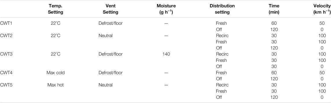
TABLE 1. Specification of the CWT test settings.

A total of 39 time series variables, measured at either 1 or 10 s intervals depending on the test facility, are divided into control (Table 2) and state (Table 3) vectors. Control variables are considered to be exogenous inputs to the simulation and are either controllable (blower amperage), uncontrolled but measurable (car velocity), or indirectly controlled (vent temperatures). State variables include personal temperatures to allow estimation of thermal comfort (e.g., via ISO 7730 or ISO 14505) and estimation of windshield fogging. Rolling means of window 50 and 5 were applied to the 1 and 10 s interval data respectively and then the 1 s data was subsampled to 10 s intervals.

TABLE 2

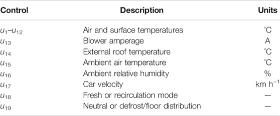
TABLE 2. Measurement variables that comprise the control vector u. The air temperatures (u₁−u₁₂) correspond to: vents at the side, central, floor, and near duct for driver and front passenger; recirculation inlet; and left, right, and central dashboard surface temperatures.

TABLE 3

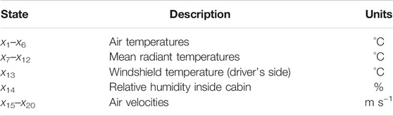
TABLE 3. Measurement variables comprising the state x. Personal variables (air and mean radiant temperature and air velocity) are measured at the head, torso, and foot locations for both driver (x₁ − x₃, x₇ − x₉, x₁₅ − x₁₇) and passenger (x₄ − x₆, x₁₀ − x₁₂, x₁₈ − x₂₀).

Figures 1, 2 show the locations for the vents and cabin sensors respectively.

FIGURE 1

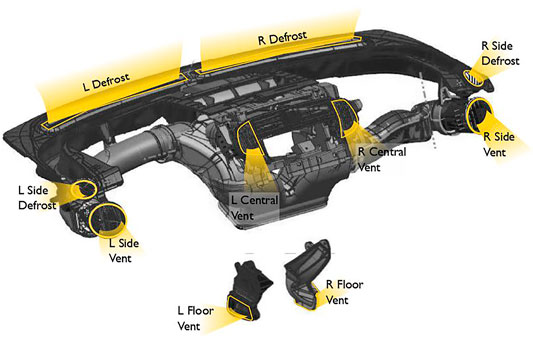
FIGURE 1. Vent outlets on instrument panel and in footwell.

FIGURE 2

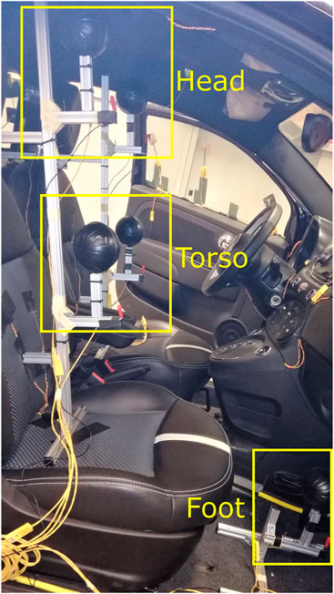
FIGURE 2. Sensors at the head, torso, and foot locations.

2.2 The Machine Learning Model

The machine learning model aims to provide a simulator that is derived without knowledge of the physical system but rather is entirely obtained from measurement data. When formulated as differential equations, thermal systems are (mainly) linear with respect to their inputs. Given a simple thermal system that involves a body (such as a container full of water) of temperature y(t), an external environment that maintains a uniform temperature y₀, and an insulating barrier (the outer wall of the container) of coefficient k, the rate of change of temperature of the body $\frac{dy}{dt}$ is proportional to the difference between the inside and outside temperature

$\frac{dy}{dt}=-k\left(y-y_0\right).(1)$

This is known as Newton’s model and forms the basis for ‘lumped’ thermal models (models where the components parts, or lumps, are considered to have a single uniform temperature). Note that the coefficient k might be expanded to consider the surface area and the unit thermal resistivity of the dividing layer. A transient simulation, given the current state y(t), must identify y(t + Δt) for some small increment in time Δt (say 1 s). An Euler simulation is a numerical approximation that assumes for a small Δt,

$\frac{\mathrm{\Delta }y}{\mathrm{\Delta }t}\approx \frac{dy}{dt}=-k\left(y-y_0\right).(2)$

Given this approximation,

$y\left(t+\mathrm{\Delta }t\right)\approx y\left(t\right)+\frac{\mathrm{\Delta }y}{\mathrm{\Delta }t}\cdot \mathrm{\Delta }t(3)$

$=y\left(t\right)-k\mathrm{\Delta }t\cdot y\left(t\right)+k\mathrm{\Delta }t{y}_0(4)$

$=\left(1-k\mathrm{\Delta }t\right)\cdot y\left(t\right)+k\mathrm{\Delta }t{y}_0(5)$

which shows that y(t + Δt) is a linear function of y(t). Therefore, assuming Δt is small, a simple linear regression between y(t) and y(t + Δt) would yield the key coefficients in what otherwise appears to be a complex relationship between the internal temperature, the external temperature, and the thermal resistivity of the dividing wall. In summary, the simple thermal problem can be simulated using a linear correspondence between the current state y(t) and the next state y(t + Δt). Finding the coefficients for such a dynamical system is termed system or model identification.

Although a simple linear correspondence may be sufficient for a simple system as the complexity of the model increases, non-linearities will appear. Furthermore, some effects, such as radiative heat transfer, are proportional to the fourth power of the difference in temperatures and thus seem to demand a more flexible modeling method. As suggested by work on non-linear autoregressive network systems, some form of neural network (NN) or recurrent neural network (RNN) may be appropriate (Ng et al., 2014a; Engel et al., 2019).

A key insight in this work is the realisation that many physical systems can be predicted using only the current state and control inputs. In some cases, the prior state is also needed (e.g., as a proxy for the velocity of a moving object where the state contains just its position). Therefore, the structure of the simulator is a transfer function of the form

${\mathbf{x}}_{t+1}=\mathbf{f}\left({\mathbf{x}}_t,{\mathbf{u}}_t,{\mathbf{x}}_{t-1}\right).$

corresponding to a network structure as shown in Figure 3.

FIGURE 3

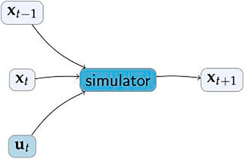
FIGURE 3. Simulator is phrased as a recursive function, which is trained with one-step examples.

2.3 Model Learning

Having preprocessed the data, random hyperparameter search is used to identify the best neural network or multilayer perceptron (MLP) structure (Aureélien, 2019). The parameter space that we have chosen to search over are:

• Number of hidden layers (0–4).

• Activation for hidden layers (ReLU, sigmoid, tanh, linear).

• Activation for final layer (linear).

• Number of nodes in each hidden layer (1–500).

• Whether a dropout regularisation, a technique where randomly selected neurons are ignored during training (Srivastava et al., 2014), is used (selected from the set 0, 0.5).

The final activation layer is chosen to be linear as this is a regression problem with real-valued outputs.

The network is learnt using TensorFlow (Abadi et al., 2015) and Keras (Chollet, 2015) with the Adam optimizer (Kingma and Ba, 2014) aiming at minimising the mean square error. From the hyperparameter space given above, 200 variants are selected at random (with uniform distribution for number of nodes). Input and outputs are rescaled to a unit range using min–max rescaling.

Two considerations are made when performing the hyperparameter search. First, the data comes in the form of groups due to the presence of five different CWT trials with varying settings. Second, shuffling in cross validation is not appropriate for time series data. In order to address these, we make use of a Time Series Group Split cross-validator. This requires that each successive training set is a superset of those before it for each of the five groups.

Model training is done in open loop, meaning the true output rather than the predicted one is used for the next step prediction (Menezes and Barreto, 2008). In order to measure the performance of our model, we utilise the mean squared error (MSE) loss function.

2.4 Linear Regression

Alongside the more complex MLPs, linear (least-squares) regression (LR) is also be considered. LR is a closed form solution to the least-squares problem whereas stochastic gradient descent (SGD) used for the MLP is iterative and approximate and thus can have a performance advantage. As with the perceptron, LR uses a minimal set of coefficients to model the system. This means that overfitting is unlikely although there may be some possibility of underfitting (not providing sufficient flexibility in the model). The simplicity of LR tends to make it robust to measurement noise although noise in sensor readings used as the independent variables causes LR to underestimate the gradient. Time series noise reduction is used to reduce this effect.

2.5 State of the Art 1D Model

Alongside the ML model, we use AMESim version 17 software (Siemens, 2018) to model the North America Fiat 500 BEV climate system. It is a programming environment developed for the object-oriented modeling of complex physical systems. The main libraries used are: thermal, thermo-hydraulic, two-phase flow, heat, and air-conditioning.

The modeling has been carried out using the bottom-up approach: starting from the basic components, the different subsystems have been assembled and then connected to each other until reaching the final system configuration. The climate system includes the following sections:

1. HVAC system, which includes the evaporator, air ducts, and Positive Temperature Coefficient electric heater, and is connected to the cabin.

2. Two-phase flow loop, which includes the compressor, the heat exchangers, and the thermal expansion valves.

3. Battery and Power Train (PWT) coolant loops which provide battery and PWT thermal management.

Each component model (i.e., compressor, evaporator, condenser, etc.) has been made filling the AMESim template with the geometrical data available from the datasheet. The template has some parameters that are calibrated using the data test recovered from the datasheet itself (i.e., the heat exchange coefficient derives from the Nusselt number calibration among the power exchanged by the heat exchanger). The developed cabin model consists of several thermal masses corresponding to the main inertial masses that interact between them by conduction and radiation and with the air by convection. The heat exchange by convection with the air depends on the air speed on the single surface. The heating and cooling modes have different airflow distributions, tri-level and only vent respectively, therefore, separate models are realized for these two functional modes. The heat exchange coefficients on surfaces are calibrated using measured data collected during the standard procedure of cabin warm-up and cooldown. Along the cabin air path (from the HVAC to the cabin), no pressure drop is considered than the airflow is imposed at the inlet of HVAC. The airflow rate is variable according to the thermal strategy adopted. The model is suitable to evaluate the electrical power consumption of the different actuators (blowerend fan on the low voltage net; the compressor and the Positive Temperature Coefficient on the HV net).

3 Results

3.1 Hyperparameter Search

The top performer is LR with MSE 0.000 047 ± 0.000 005 7 for next step (10 s) predictions of min-max rescaled data. Due to the rescaling required for the neural network, the MSE is already normalised. Thus, it translates to a NRMSE of $\sqrt{0.00024}\frac{100}{1}\%$ = 0.68% over 10 s. Note that the prediction error for several hours of simulation is likely to be larger.

Figure 4 provides an overview of the results from the hyperparameter search, detailed in Section 2.3. The main results shown here are that for those network structures that perform poorly, dropout helps considerably. Dropout is a regularisation technique that disables connections in the network with a fixed probability. This approach is often helpful in dealing with large, highly correlated inputs by making the network less reliant on individual inputs and thus more robust.

FIGURE 4

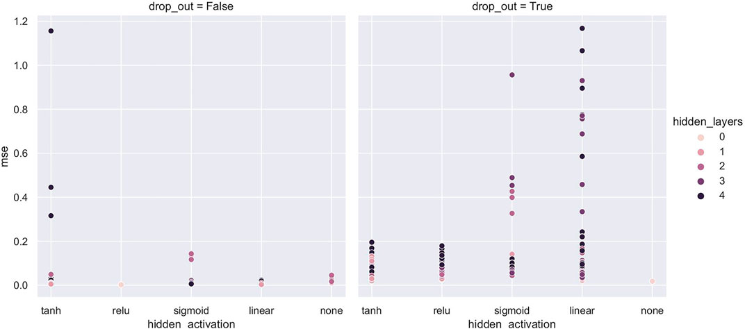
FIGURE 4. Overview of hyperparameter search.

The top 10 performers of the hyperparameter search are shown in Table 4. The MSE is given as mean ± standard deviation over the Time Series Group Split cross-validation. One of the top performers is a simple perceptron system (single layer of linear activation). This is equivalent to a linear function between inputs and outputs, which thus suggests that linear regression (LR) may also be effective.

TABLE 4

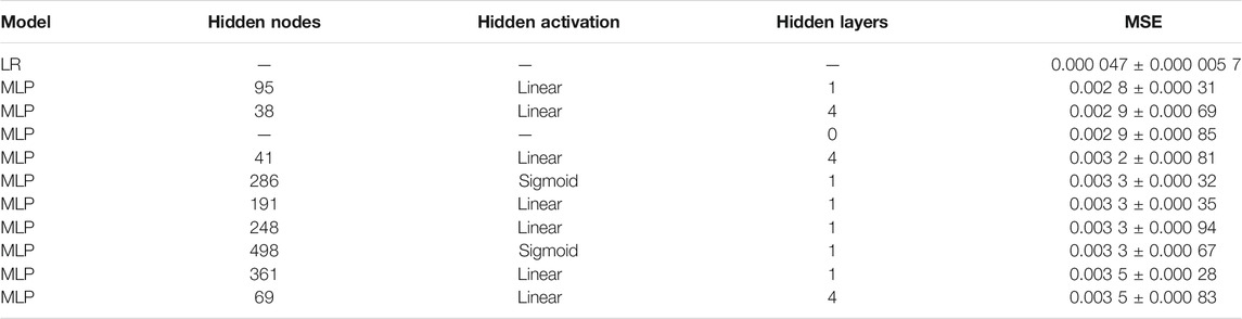
TABLE 4. Linear regression and the top 10 MLP from the hyperparameter search results where the final activation is linear and there is no dropout.

Linear regression does not require rescaled data but, for the purposes of comparison, cross validation LR on rescaled data gave an MSE of 0.000 047 ± 0.000 005 7 which outperforms the top performing MLP. Due to LR being a more robust model and the fact that thermal systems are mainly linear, LR is chosen as the model for this data.

3.2 Evaluation as Long-Run Simulator

3.2.1 Simulation Results Comparing Simulator With Original Data

Figure 5 shows a comparison of simulation output with measurement data for the air temperature at the driver’s head position during CWT1. The correspondence is remarkable since there is no divergence between two curves - there is only a small error between them - even over the extended period of the test (around 3 h). Furthermore, the temperatures vary over a large range during the trial from almost 0°C at the beginning to a peak of nearly 30°C.

FIGURE 5

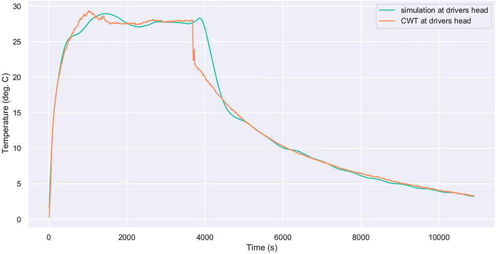
FIGURE 5. Comparison of simulation produced curve for the air temperature at the driver’s head versus measurement data from CWT1 (without smoothing) giving an RMSE of 0.78. The trial settings are 22°C on defrost/floor with fresh distribution at 50 km h⁻¹ for 60 min, then all settings are switched off for 120 min.

Other sensor modalities are reproduced with similar accuracy. Again, this is striking as the relative humidity varies over a wide range during the trial. The simulator manages to track it almost perfectly just on the basis of the initial state and the control inputs.

Air velocity measurements tend to vary considerably. These measurements are smoothed during processing and thus the simulator produces a smooth estimate of the air velocity. The correspondence here is quite consistent through the whole period.

3.2.2 Differences Between Head, Torso, and Foot Temperatures

A key benefit of the ML-based simulation approach is the ability to differently estimate different parts of the cabin space. For example, the temperature at the head may be much hotter than the footwell and this difference affects thermal comfort. Therefore, it is interesting to see whether the simulation is able to independently and differently track the air temperature (for example) at the head, torso and foot. Figures 6, 7 demonstrate that this tracking is very good. In particular, notice that the footwell is higher than the head and torso locations during the first part of the trial while the long term progression (where the HVAC was turned off after 4,000 s) ended with clearly separate temperatures for the three locations and that all were correctly predicted by the simulator.

FIGURE 6

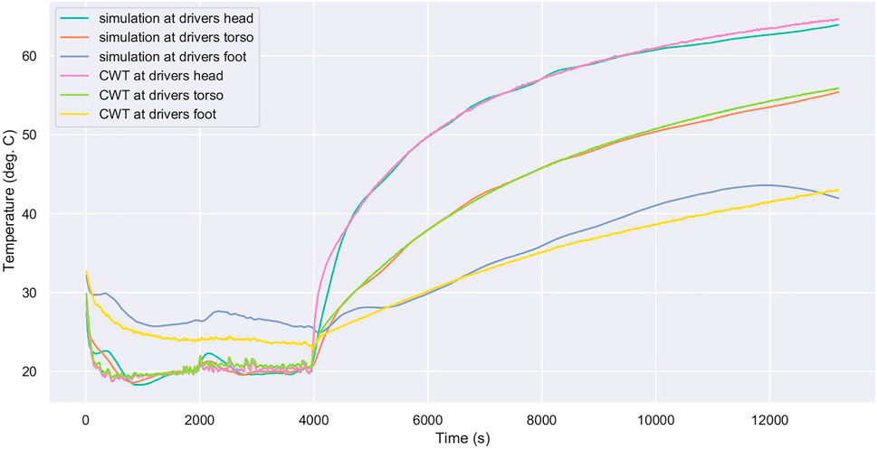
FIGURE 6. ML-simulator correctly and independently tracks driver’s head, chest, and foot temperatures over a 3 h trial (CWT2) with only small errors. The trial settings are 22°C with vents set to neutral and recirculated distribution at 100 km h⁻¹ for 30 min, then switching to fresh distribution for 30 min, before switching all settings off for 120 min.

FIGURE 7

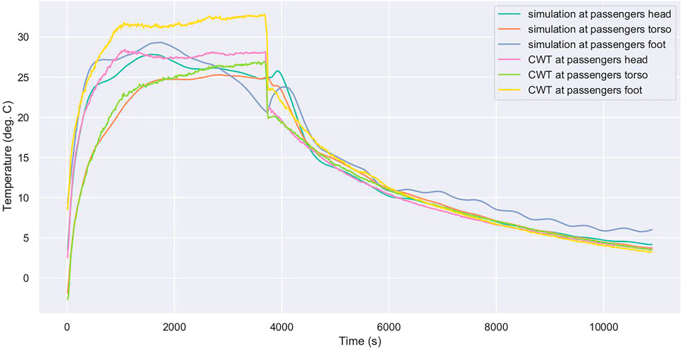
FIGURE 7. Passenger side air temperatures are reasonably accurately tracked with clear differences during the early phase between head, torso, and foot for trial CWT1. The trial settings are 22°C on defrost/floor with fresh distribution at 50 km h⁻¹ for 60 min, then all settings are switched off for 120 min.

The temperature predictions in the footwell are not quite as accurate as the predictions for the head and torso during the beginning of the trial (0, − , 4,000 s). A reason for this may be that the model has not captured some characteristics of the footwell, such as the fact that the area is more enclosed and therefore may be more insulated. This may not be detrimental as a perfect simulation may not be needed (Ha and Schmidhuber, 2018).

3.2.3 Examples Showing Room for Improvement

Figure 8 shows some response differences for air temperature at the driver’s head in the simulator compared to the data from CWT3. Note that the vertical range is small and this may appear to magnify errors. A striking aspect of this result is that the final temperature converged upon is very close to the true final temperature. Another example is the windshield temperature simulation for CWT3, shown in Figure 9. Here the temperatures are quite stable during the CWT trial but vary considerably in the simulation. Again, the vertical range is small but the error is up to 3 K.

FIGURE 8

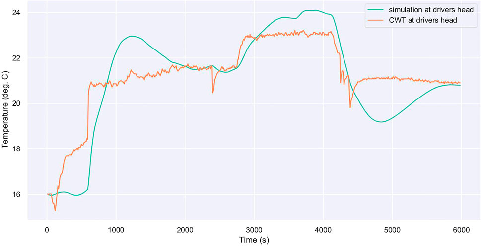
FIGURE 8. Comparison of measurement and simulated data for CWT3 air temperature at the driver’s head. The trial settings are 22°C with vents set to defrost/floor with recirculated distribution and 140 g h⁻¹ of moisture at 100 km h⁻¹ for 30 min, then switching to fresh distribution for 30 min, before switching all settings off for 30 min.

FIGURE 9

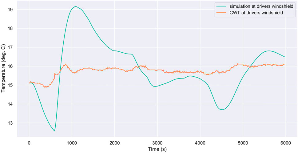
FIGURE 9. Comparison of measurement and simulated data for CWT3 windshield temperature driver’s side. The trial settings are 22°C with vents set to defrost/floor with recirculated distribution and 140 g h⁻¹ of moisture at 100 km h⁻¹ for 30 min, then switching to fresh distribution for 30 min, before switching all settings off for 30 min.

For Figures 8, 9, recall that CWT3 is the only trial with moisture added into the cabin. The average NRMSE across all sensors for the full trial duration is 0.16 (or 16%) for CWT3, whereas the other four CWT trials are in the range of 0.041 (4.1%) to 0.082 (8.2%). It is possible that providing more CWT trial data where moisture is added into the cabin to train the model on may help to improve these predictions.

3.2.4 NRMSE Results

Rather than trying to understand the accuracy of the simulation based on examining individual graphs, it is generally more appropriate to summarise the error in terms of the RMSE or NRMSE. Table 5 shows results obtained by running the simulator for each of the CWT trials. The RMSE and NRMSE shown here is the mean ± the standard deviation over the 5 trials. Note that NRMSE is shown as a proportion rather than a percentage. For example, an NRMSE of 0.004 corresponds to 0.4%. The RMSE and NRMSE values here are for the full trials (around 3 h) and thus will be somewhat larger than the 10 s prediction RMSE or corresponding MSE used during training. The units for the RMSE depend on the sensor, as specified in Table 3. Note that the displayed decimal places are adjusted according to the standard deviation.

TABLE 5

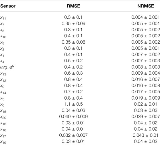
TABLE 5. Performance of ML model in terms of error for each sensor ordered according to mean NRMSE. Average air temperature (avg_air) is based on comparing the average of head, torso and foot air temperatures for driver and front passenger with that of the simulated values.

The average NRMSE performance over all sensors over the full trial duration is 0.018 (or 1.8%), which is comparable but slightly larger than the 10 s NRMSE (1.5%). The average air temperature RMSE is 0.4 K or 0.8%.

3.2.5 Compute Performance

Calculating a single time step (10 s) with the simulator developed in this work is extremely fast. The reason for this fast performance is that the calculation can be performed with a single matrix multiplication. Also, LR, unlike the neural network, does not require rescaling of inputs and outputs. On a PC with Intel(R) Core(TM) i7-4790 CPU at 3.60 GHz processor, 1,000, ×, 3 h simulations were calculated in 59.3 s. This corresponds to 0.005 44 ms s⁻¹ (elapsed time per simulation second).

Compute performance becomes critical when attempting to use machine learning to optimise a control algorithm. In past work, around 9 years of simulated time was required to find the optimal control strategy. The time to compute 9 years of simulated time using this simulator is around 25 min.

3.2.6 Discussion

These results show high accuracy for this simulator over all the sensors. The smallest errors are less than the expected error in the thermocouple sensor while the largest errors (around 0.04 m s⁻¹ or 4% of the range) are within 5% of the accuracy of the high-level model. The results reflect that short-term errors tend to disappear over time. This is surprising because, in many simulations, small errors accumulate when producing a simulation that runs over an extended period. This reflects the relative simplicity of the model causing it to be extremely robust. Possible threats to validity of the LR simulation results are as follows:

• These results are specific to the range of parameters varied during the CWT trials. For example, only 2 distribution modes were switched between—it would not be possible to use this simulator to simulate other distribution modes.

• Similarly, it is expected to add radiant panels and other options that will impact the thermal dynamics. These trials do not include such features and thus could not be used to simulate them. The aim, however, is to apply this method to CFD-based data, which would allow the inclusion of these extra features.

• A better estimate of the performance on unseen data might be possible using k-fold cross-validation. Since the full data-set was used to both learn the linear regression coefficients and to assess performance, the true performance on unseen data may be slightly worse than estimated here. Note, however, that overfitting is unlikely for this method.

3.3 Comparative Performance of 1D and Machine Learning Models

3.3.1 Accuracy

The average NRMSE over all sensors being estimated for the ML-based simulator is 1.8%. The best estimated sensor (mean radiant temperature at passenger’s torso) has an NRMSE of 0.4% while the worst (air velocity at passenger’s torso) has a 4.0% NRMSE. The error of the estimate of the average air temperature over the front bench of the car cabin is 0.4 K (0.8%).

The 1D model NRMSE is 1.5% for the temperature. When the AC loop is on, the model performs about 3% for the high pressure and 6% for the low pressure.

3.3.2 Computational Speed

To compare the computational speed, we look at the amount of elapsed time to compute 1 s of simulated time. The results for 1D simulation models are:

• 7.6 ms s⁻¹ in warm up protocol.

• 250 ms s⁻¹ in cool down protocol.

The result for the ML model is:

• 0.005 44 ms s⁻¹.

Note that the ML-based simulation does not attempt to simulate the cooling loop but does simulate different parts of the car cabin (driver and passenger’s head, torso and foot).

Based on the above results, the speed-up for the ML-based simulator compared with the 1D simulation (during warm up) is 1400-fold.

3.3.3 Capability

The two simulators have different sets of capabilities and this should be taken into account when considering other performance aspects.

The ML-based simulator has certain capabilities that are not available in the 1D simulator:

• It can provide properties needed to make use of a holistic comfort model for both front bench occupants. Specifically, it estimates temperature, mean radiant temperature, and air velocity at the head, torso, and foot positions for both occupants.

• It can provide properties needed for estimating safety in terms of windshield fogging. Specifically, it estimates windshield glass temperature and relative humidity.

The 1D simulator, on the other hand, has capabilities not available in the ML simulator:

• It simulates the HVAC system more fully, including the AC loop, rather than requiring the air vent temperature as input. Note that the ML simulator does simulate the blower.

• It is a physics-based simulation and thus is likely to generalise more readily to circumstances not seen in the CWT trials.

• It supports additional components, such as the radiant panels.

Due to these differences in capabilities, the choice of simulator will depend on the application.

4 Discussion

The primary aim of simulation models for car HVAC systems is to ensure that components are sufficiently powerful to cope with the expected range of conditions and to ensure that the cabin is cooled or warmed sufficiently quickly. For this reason, relatively simple 1D thermal models are commonplace in industry (Doyle and Muneer, 2019; Marcos et al., 2014). More recently, the energy cost of the climate system has become more important (Lajunen, 2017; Kambly and Bradley, 2014) along with the realisation that thermal comfort is not simply a function of air temperature. As a result, other measurements have been considered, such as mean radiant temperature (Khatoon and Kim, 2020) and air velocity Kamar et al. (2013).

There is an abundance of research on thermal models for commercial or residential buildings (Afram et al., 2017; Kusiak et al., 2014), with other similar applications including personal space heaters (Katić et al., 2018), high performance computers (Zhang et al., 2018), and water heating systems (Kalogirou et al., 1999). Work has also been done using artificial neural networks in automotive applications with the focus mainly on the automotive air conditioning system. Some models are used to predict system performance and cooling capacity (Hosoz and Ertunc, 2006; Kamar et al., 2013; Datta et al., 2019). Other work, such as that by Ng et al. (2014b), makes use of MLP and radial basis network with experimental data to predict average cabin temperature. Our purpose is to estimate thermal comfort using the ISO 14505 model, which requires 3 modalities (temperature, mean radiant temperature, and air velocity) for at least 3 locations (head, torso, foot) for each passenger (a total of 3 × 3 × 4 variables). Furthermore, we need to check if the windows get fogged and so we also need cabin relative humidity and windshield temperature. Predicting so many variables is a big step up from predicting a single average cabin temperature but this work shows that it is possible.

5 Conclusion

The key results are:

1. The ML cabin model has an average NRMSE over all sensors of 1.8%. The RMSE for the average air temperature for the front bench is 0.4 K (0.8%) over all trials.

2. The ML cabin model computes a second of simulation time in 0.005 44 ms.

3. The 1D cabin model predicts the cabin average air temperature within ±1 K (1.52%).

4. The 1D cabin model predicts AC pressure with an average error less than 0.6 bar (3%) at high pressure and 0.1 bar (6%) (steady state) at low pressure. The 1D cabin model computes a second of simulation time in 0.25 s (worst case—when the AC compressor is on) or 0.0076 s (AC compressor off).

The best performing machine-learnt simulator is based on linear regression and gives an average, whole trial NRMSE of 1.8%. The simulator closely tracks thermal, relative humidity, and air velocity dynamics within the cabin and clearly demonstrates the viability of the method. This simulator provides a solid basis for work where it is not necessary to add components, such as radiant panels. Furthermore, this work is remarkable in that it provides a simulator that is capable of accurately simulating the thermal dynamics at multiple car seating positions and to do so with a compute performance that is much faster than traditional 1D approaches. This opens the way for numerical optimisation approaches that were previously considered infeasible to build car cabin HVAC controllers and redesign the car cabin features. Future work is required to provide data that can enable simulation of optional components including radiant panels, heated seats, and special glazing.

The ML-based simulator is sufficiently fast and accurate to suggest that this is a promising method. The 1D simulator, being physics-based, may still be preferred for some applications.

In order to make use of the ML-based simulator, additional work is needed, as follows:

1. A separate simulation of the HVAC system is needed to provide vent outlet temperatures.

2. To properly simulate components, such as the radiant panels, further simulation data are needed. This data might be produced based on the computational fluid dynamics simulation, for example.

3. More information could also be included in the model such as contact heat (i.e., heated seats) and the accumulation of CO₂ in the cabin (Angelova et al., 2019).

Minimising unnecessary energy consumption is central to the design of modern electric vehicles and the car cabin’s heating and cooling system is the car’s largest auxiliary load. However, personal comfort depends on this HVAC system and is critical to customer satisfaction, while some of this functionality is also needed for safety (such as defogging the windscreen). Therefore, it is important to minimise energy use under the constraint of maintaining acceptable comfort and safety. The methods presented in this paper model the thermal environment within a car cabin to help identify whether comfort and safety requirements can be met and at what energy cost.

Data Availability Statement

The datasets presented in this article are not readily available because it is private data from CRF. Requests to access the datasets should be directed to Brandi Jess, jessb@uni.coventry.ac.uk.

Author Contributions

MR and AM built the 1D model. BJ, JB, and KG contributed to the ML model. JB wrote the first draft of the manuscript. BJ reran analysis and wrote sections of the manuscript. EG provided feedback on writing. All authors contributed to manuscript revision, read, and approved the submitted version.

Funding

This research is a part of the DOMUS project, which received funding from the European Union’s Horizon2020 research and innovation programme under Grant Agreement No. 769902. Further information can be found here: DOMUS project.

Conflict of Interest

MR and AM were employed by the company Centro Ricerche Fiat S.C.p.A.

The remaining authors declare that the research was conducted in the absence of any commercial or financial relationships that could be construed as a potential conflict of interest.

Publisher’s Note

All claims expressed in this article are solely those of the authors and do not necessarily represent those of their affiliated organizations, or those of the publisher, the editors and the reviewers. Any product that may be evaluated in this article, or claim that may be made by its manufacturer, is not guaranteed or endorsed by the publisher.

Acknowledgments

We would like to thank Fabrizio Mattiello (CRF) for his supervision of the experimental work in the CWT on the baseline vehicle which provided the data used in this work.

References

Abadi, M., Agarwal, A., Barham, P., Brevdo, E., Chen, Z., Citro, C., et al. (2015). TensorFlow: Large-Scale Machine Learning on Heterogeneous Systems. arXiv, 1–19. arXiv:1603.04467.

Google Scholar

Afram, A., Janabi-Sharifi, F., Fung, A. S., and Raahemifar, K. (2017). Artificial Neural Network (ANN) Based Model Predictive Control (MPC) and Optimization of HVAC Systems: A State of the Art Review and Case Study of a Residential HVAC System. Energy and Buildings 141, 96–113. doi:10.1016/j.enbuild.2017.02.012

CrossRef Full Text | Google Scholar

Angelova, R. A., Markov, D. G., Simova, I., Velichkova, R., and Stankov, P. (2019). Accumulation of Metabolic Carbon Dioxide (CO2) in a Vehicle Cabin. IOP Conf. Ser. Mater. Sci. Eng. 664, 012010. doi:10.1088/1757-899x/664/1/012010

CrossRef Full Text | Google Scholar

Aureélien, G. (2019). Hands-on Machine Learning with Scikit-Learn and TensorFlow: Concepts, Tools, and Techniques to Build Intelligent Systems. Sebastopol, California, United States: OReilly.

Google Scholar

Campbell, P. (2020). Uk Set to Ban Sale of New Petrol and Diesel Cars from 2030. Auto Express. 14-Nov-2020.

Google Scholar

Chollet, F. (2015). Keras. San Francisco, California, United States: GitHub. Available at: https://github.com/fchollet/keras.

Google Scholar

Datta, S. P., Das, P. K., and Mukhopadhyay, S. (2019). An Optimized ANN for the Performance Prediction of an Automotive Air Conditioning System. Sci. Technol. Built Environ. 25, 282–296. doi:10.1080/23744731.2018.1526014

CrossRef Full Text | Google Scholar

Doyle, A., and Muneer, T. (2019). Energy Consumption and Modelling of the Climate Control System in the Electric Vehicle. Energy Exploration & Exploitation 37, 519–543. doi:10.1177/0144598718806458

CrossRef Full Text | Google Scholar

Engel, P., Meise, S., Rausch, A., and Tegethoff, W. (2019). “Modeling of Automotive HVAC Systems Using Long Short-Term Memory Networks,” in Proceedings of the ADAPTIVE 2019: The Eleventh International Conference on Adaptive and Self-Adaptive Systems and Applications, Venice, Italy, May 2019, 48–55.

Google Scholar

Farrington, R., and Rugh, J. (2000). “Impact of Vehicle Air-Conditioning on Fuel Economy, Tailpipe Emissions, and Electric Vehicle Range,” in Earth Technologies Forum (Washington DC: GRSS). National Renewable Energy Laboratory, 1–10.

Google Scholar

Ha, D., and Schmidhuber, J. (2018). “Recurrent World Models Facilitate Policy Evolution,” in Proceedings of the Advances in Neural Information Processing Systems 31, Montréal, Canada, December, 2018 (New York, United States: Curran Associates, Inc.), 2451–2463. Available at: https://worldmodels.github.io.

Google Scholar

Hosoz, M., and Ertunc, H. M. (2006). Artificial Neural Network Analysis of an Automobile Air Conditioning System. Energ. Convers. Manage. 47, 1574–1587. doi:10.1016/j.enconman.2005.08.008

CrossRef Full Text | Google Scholar

IEA (2020). Global EV Outlook 2020. Tech. Rep. Paris: IEA.

Google Scholar

Kalogirou, S. A., Panteliou, S., and Dentsoras, A. (1999). Modeling of Solar Domestic Water Heating Systems Using Artificial Neural Networks. Solar Energy 65, 335–342. doi:10.1016/S0038-092X(99)00013-4

CrossRef Full Text | Google Scholar

Kamar, H. M., Ahmad, R., Kamsah, N. B., and Mohamad Mustafa, A. F. (2013). Artificial Neural Networks for Automotive Air-Conditioning Systems Performance Prediction. Appl. Therm. Eng. 50, 63–70. doi:10.1016/j.applthermaleng.2012.05.032

CrossRef Full Text | Google Scholar

Kambly, K. R., and Bradley, T. H. (2014). Estimating the HVAC Energy Consumption of Plug-In Electric Vehicles. J. Power Sourc. 259, 117–124. doi:10.1016/j.jpowsour.2014.02.033

CrossRef Full Text | Google Scholar

Katić, K., Li, R., Verhaart, J., and Zeiler, W. (2018). Neural Network Based Predictive Control of Personalized Heating Systems. Energy and Buildings 174, 199–213. doi:10.1016/j.enbuild.2018.06.033

CrossRef Full Text | Google Scholar

Khatoon, S., and Kim, M.-H. (2020). Thermal Comfort in the Passenger Compartment Using a 3-D Numerical Analysis and Comparison with Fanger's Comfort Models. Energies 13, 690. doi:10.3390/en13030690

CrossRef Full Text | Google Scholar

Kingma, D. P., and Ba, J. (2014). Adam: A Method for Stochastic Optimization. arXiv, 1–15. arXiv:1412.6980.

Google Scholar

Kusiak, A., Xu, G., and Zhang, Z. (2014). Minimization of Energy Consumption in HVAC Systems with Data-Driven Models and an interior-point Method. Energ. Convers. Manage. 85, 146–153. doi:10.1016/j.enconman.2014.05.053

CrossRef Full Text | Google Scholar

Lajunen, A. (2017). Energy Efficiency and Performance of Cabin Thermal Management in Electric Vehicles. Technical Papers 2017-01-0192. Warrendale, Pennsylvania, United States: SAE International. doi:10.4271/2017-01-0192

CrossRef Full Text | Google Scholar

Marcos, D., Pino, F. J., Bordons, C., and Guerra, J. J. (2014). The Development and Validation of a thermal Model for the Cabin of a Vehicle. Appl. Therm. Eng. 66, 646–656. doi:10.1016/j.applthermaleng.2014.02.054

CrossRef Full Text | Google Scholar

Menezes, J. M. P., and Barreto, G. A. (2008). Long-term Time Series Prediction with the NARX Network: An Empirical Evaluation. Neurocomputing 71, 3335–3343. doi:10.1016/j.neucom.2008.01.030

CrossRef Full Text | Google Scholar

Ng, B. C., Darus, I. Z. M., Jamaluddin, H., and Kamar, H. M. (2014a). Application of Adaptive Neural Predictive Control for an Automotive Air Conditioning System. Appl. Therm. Eng. 73, 1244–1254. doi:10.1016/j.applthermaleng.2014.08.044

CrossRef Full Text | Google Scholar

Ng, B. C., Darus, I. Z. M., Jamaluddin, H., and Kamar, H. M. (2014b). Dynamic Modelling of an Automotive Variable Speed Air Conditioning System Using Nonlinear Autoregressive Exogenous Neural Networks. Appl. Therm. Eng. 73, 1255–1269. doi:10.1016/j.applthermaleng.2014.08.043

CrossRef Full Text | Google Scholar

Siemens (2018). Simcenter Amesim 17. Munich, Germany: Seimens.

Google Scholar

Srivastava, N., Hinton, G., Krizhevsky, A., Sutskever, I., and Salakhutdinov, R. (2014). Dropout: A Simple Way to Prevent Neural Networks from Overfitting. J. Machine Learn. Res. 15, 1929–1958. doi:10.5555/2627435.2670313

CrossRef Full Text | Google Scholar

UK Government (2020). 2019 National Travel Survey Factsheets. Tech. Rep. Horseferry Road, London: Department for Transport. Available at: https://www.gov.uk/government/statistics/national-travel-survey-2019.

Google Scholar

Zhang, K., Guliani, A., Ogrenci-Memik, S., Memik, G., Yoshii, K., Sankaran, R., et al. (2018). Machine Learning-Based Temperature Prediction for Runtime Thermal Management across System Components. IEEE Trans. Parallel Distrib. Syst. 29, 405–419. doi:10.1109/TPDS.2017.2732951

CrossRef Full Text | Google Scholar