A numerical investigation exploring the potential role of porous fencing in reducing firebrand impingement on homes

Firebrand impingement is a leading cause of home ignitions from wildland fire. The use of porous fencing has recently been proposed as a potential method for mitigating firebrand impingement on homes. A porous fence can act as a windbreak to alter the near-surface flow and induce particle deposition, as demonstrated in other applications, such as the use of snow fences to protect roadways from drifting snow. Conservation advocates have proposed the use of fire-resistant vegetation to act as a fence upwind of homes or subdivisions. Porous fences could also be constructed from fire-resistant materials such as metal, rock, or composites. This numerical investigation of the effectiveness of porous fencing to reduce firebrand impingement on homes conducted a series of experiments to explore the effect of porous fencing on the near-surface flow field and firebrand transport downwind of the fence. We also evaluated the sensitivity of the results to various fence, flow, and firebrand properties, including fence height, fence porosity, wind speed, firebrand source location, and firebrand size. To our knowledge, this is the first study to investigate the concept of using a fence to induce firebrand deposition upwind of homes. Our results showed that porous fencing can reduce firebrand impingement on homes by up to 35% under certain conditions; however, fencing can also increase impingement on homes. The mitigation effectiveness depended on the proximity of the firebrand source, distance between the fence and home as a function of fence height, wind speed, and firebrand size. A series of key findings and recommendations are provided.

Introduction

Firebrand impingement is a leading cause of home ignitions from wildland fires (Cohen, 2000; Cohen and Stratton, 2008; Maranghides and Mell, 2011). Methods to reduce such ignitions include home hardening, water spraying systems, and improving defensible space around the home and in regions extending from the home (e.g., fuel thinning to modify potential fire behavior). Homes located within the wildland urban interface (WUI) are most at risk of ignition from wildland fire. Homes located in fire-prone areas that are also subject to frequent high winds (e.g., Santa Ana winds in southern California) are particularly at risk as ignitions can spread quickly and exhibit extreme fire behavior under high winds. While current California Department of Forestry and Fire Protection standards (CAL FIRE, 2022) restrict fuels within 30 m of the home, many local county fire departments in the US require homeowners to reduce fuels within 60 m of the home, depending on the type of fuel and the terrain surrounding the home (Nader et al., 2007). The requirements can also include a minimum spacing between different heights of fuels for various slope angles, decreased ground fuels, and increased irrigation at various distances from the home. Recommendations for the following are provided in some cases: specific types, sizes, and species of vegetation; locations of fences and yard accessories around the home; home construction materials; vent filters; gutter protection; and maintenance of the vegetation, home exterior, and surrounding defensible space (e.g., Nader, 2007; RCDSMM, 2022).

The 2018 Woolsey Fire near Santa Monica, California destroyed 1,643 structures and stimulated interest in a potential new approach of using vegetation fences to protect homes from firebrand impingement. The Woolsey Fire started on the afternoon of November 8, 2018, just north of Calabasas, California (Los Angeles County, 2019). Ultimately, the Woolsey Fire burned 96,949 acres across two counties, with most of the fire activity occurring in the first 30 h. The fire occurred under a Santa Ana wind event (a strong katabatic wind that frequently occurs in the mountain passes of southern California due to high pressure to the east in the Great Basin region of the US), with sustained winds of 13 m/s and gusts up to 27 m/s. The fire spread rapidly under these wind conditions through flashy chaparral and grass fuels. The fire spotted across multiple roads and highways, indicating that spotting via firebrand transport ahead of the main fire front was a major contributor to fire spread. Numerous images online demonstrate the presence and role of firebrands, including images of palm trees torching and spewing firebrands, firebrand showers passing through neighborhoods, and burning boats in the middle of a lake, apparently ignited by firebrands (e.g., Taylor, 2018).

The substantial short- and medium-range spotting associated with the Woolsey Fire and the large number of structures destroyed prompted consideration of the use of vegetation fences to alter the flow near structures to induce firebrand deposition upwind of and reduce firebrand impingement on homes. This concept has been used successfully in other applications, such as protecting roads from drifting snow with upwind snow fences (Liu et al., 2016; Du et al., 2017) and reducing near-road pollution via vegetation fences (Tong et al., 2016). Conservation advocates have proposed revisions of existing defensible space guidelines to potentially include the scope for retaining some vegetation to serve as a barrier to wind and firebrand transport. One obvious risk is that the vegetation fences or litter deposited by them could ignite and become an additional threat much closer to the home. Proponents suggest that fences could be designed using well-maintained and well-irrigated fire-resistant species to minimize this risk. Alternatively, fences constructed from other fire-resistant materials (e.g., metal, rock, or composite fencing) could be considered.

This study explored the potential of porous fences to alter the near-surface flow field and reduce firebrand impingement on homes from short-range spotting (i.e., spotting distances 10s to 100s of meters ahead of the flaming front). We conducted a series of numerical experiments to test the potential effectiveness of this concept. The experiments were designed with a porous fence intended to represent a row of trees; however, the results are applicable to fences constructed from other materials so long as the fence can be approximated by the porous media representation described in our numerical setup.

Methods

We conducted a series of numerical experiments to assess the feasibility of porous fencing for reducing firebrand impingement on homes. These experiments were performed using the open-source computational fluid dynamics toolbox, OpenFOAM, version 8 (Weller et al., 1998; www.openfoam.org).

The wind field was simulated using a Reynolds-averaged Navier-Stokes (RANS) model with k-epsilon turbulence closure. The flow model setup was identical to the RANS solver described in Wagenbrenner et al. (2019). The model boundary conditions were set to ensure the horizontal homogeneity of the flow solution over flat terrain, as described in Richards and Norris (2011).

The RANS equations are

$\frac{\partial {\overline{u}}_i}{\partial x_i}=0,(1)$

$\frac{\partial \left({\overline{u}}_j{\overline{u}}_i\right)}{\partial x_j}=-\frac{1}{\rho }\frac{\partial \overline{p}}{\partial x_i}+\frac{\partial }{\partial x_j}\left(v\left[\frac{\partial {\overline{u}}_i}{\partial x_j}+\frac{\partial {\overline{u}}_j}{\partial x_i}\right]\right)+\frac{\partial }{\partial x_j}\left(-\rho \overline{u_i^{\prime }{u}_j^{\prime }}\right),(2)$

where ${\overline{u}}_i$ and ${\overline{u}}_j$ are the time-averaged velocity components in the $i$ and $j$ coordinate directions, $u_i^{\prime }$ and $u_j^{\prime }$ are the instantaneous velocity components in the $i$ and $j$ coordinate directions, $\overline{p}$ is the time-averaged pressure, $\rho$ is the density, and $v$ is the laminar viscosity. The two-equation k-epsilon turbulence model introduces a turbulent viscosity term, $v_t$, to model the contribution of the instantaneous velocity components.

$\frac{\partial \left({\overline{u}}_j{\overline{u}}_i\right)}{\partial x_j}=-\frac{1}{\rho }\frac{\partial \overline{p}}{\partial x_i}+\frac{\partial }{\partial x_j}\left(\left(v+v_t\right)\left[\frac{\partial {\overline{u}}_i}{\partial x_j}+\frac{\partial {\overline{u}}_j}{\partial x_i}\right]\right).(3)$

The turbulent viscosity is calculated as

$v_t=C_{\mu }\frac{k^2}{\epsilon },(4)$

where $C_{\mu }$ is a constant equal to 0.09 (Richards and Norris, 2011), $k$ is the turbulent kinetic energy (TKE), and $\epsilon$ is the dissipation of TKE. Two additional transport equations are solved for k and $\epsilon$.

$\frac{\partial \left(k{\overline{u}}_i\right)}{\partial x_i}=\frac{\partial }{\partial x_j}\left[\frac{v_t}{{\sigma }_k}\frac{\partial k}{\partial x_j}\right]+P-\epsilon ,(5)$

$\frac{\partial \left(\epsilon {\overline{u}}_i\right)}{\partial x_i}=\frac{\partial }{\partial x_j}\left[\frac{v_t}{{\sigma }_{\epsilon }}\frac{\partial \epsilon }{\partial x_j}\right]+C_{\epsilon 1}\frac{P\epsilon }{k}-C_{\epsilon 2}\frac{{\epsilon }^2}{k}.(6)$

The constants ${\sigma }_k$, ${\sigma }_{\epsilon }$, $C_{\epsilon 1}$, and $C_{\epsilon 2}$ are equal to 1.0, 1.3, 1.44, and 1.92, respectively (Richards and Norris, 2011). $P$ is the production of TKE and $S_{ij}$ is the mean strain rate tensor, defined as

$P=2v_t{S}_{ij}{S}_{ij},(7)$

$S_{ij}=\frac{1}{2}\left(\frac{\partial {\overline{u}}_i}{\partial x_j}+\frac{\partial {\overline{u}}_j}{\partial x_i}\right).(8)$

The inlet boundary conditions are

$U=\frac{u_{*}}{\kappa }\mathit{ln}\left(\frac{z}{z_0}\right),(9)$

$k=\frac{u_{*}^2}{\sqrt{C_{\mu }}},(10)$

$\epsilon =\frac{u_{*}^3}{\kappa z},(11)$

where the friction velocity is calculated as

$u_{*}=\frac{\kappa U_h}{\mathit{ln}\left(\frac{h}{z_0}\right)},(12)$

and $U_h$ is the specified input wind velocity at a specified reference height, $h$, above the ground, $z_0$ is the roughness length, $z$ is the height above ground, and $\kappa$ is the von Karman constant set to 0.41. The ground, outlet, and top boundary conditions are set as in Wagenbrenner et al. (2019) according to the recommendations from Richards and Norris (2011). This setup is representative of neutral atmospheric stability, which is a good approximation of the high-wind atmospheric conditions most conducive to firebrand transport.

Vegetation was represented in the simulations as porous media regions in the domain. A source term was added to the momentum, $k$, and $\epsilon$ equations to represent the effects of vegetation in the flow. This is a common way of representing the effects of vegetation on a flow field (e.g., Dalpe and Masson, 2009; Gao et al., 2018). Eqs 13–15 show the source terms, where $S_u$ is that added to the momentum equation (Eq. 3), $S_k$ is that added to the $k$ equation (Eq. 5), and $S_{\epsilon }$ is that added to the $\epsilon$ equation (Eq. 6).

$S_u=-\rho C_{d}LAD\left|U\right|U,(13)$

$S_k=\rho C_{d}LAD\left({\beta }_p{\left|U\right|}^3-{\beta }_{d}k\left|U\right|\right),(14)$

$S_{\epsilon }=\rho C_{d}LAD\frac{\epsilon }{k}\left(C_{\epsilon 4}{\beta }_p{\left|U\right|}^3-C_{\epsilon 5}{\beta }_{d}k\left|U\right|\right).(15)$

$C_d$ is the drag coefficient for the porous object in the flow; $LAD$ is the leaf area density, which is a measure of the porosity of the porous object in the flow; and ${\beta }_p$, ${\beta }_d$, $C_{\epsilon 4}$, and $C_{\epsilon 5}$ are constants equal to 1.0, 5.03, 0.78, and 0.78, respectively (Dalpe and Masson, 2009; Segersson et al., 2017). $C_d$ and $LAD$ were combined to form a new variable, $b$, which we called the blockage coefficient, where $b=C_d*LAD$. $C_d$ was held at a constant value of 0.5 and b was approximated as described in Mueller (2012). The porous objects were sized such that they were divided evenly into the cells of the computational domain and b was set to a constant value throughout the porous region for each simulation. This porous media representation is a well-accepted method to account for the effects of vegetation or other porous objects on the momentum and turbulence of the flow (Dalpe and Masson 2009; Bitog et al., 2012; Salim et al., 2015).

An impervious block representing a house was inserted into the flow. Each surface of the block was treated as a rough wall. The dimensions of the house were 15 m × 15 m x 9.1 m. Although this is a geometrically simple representation, it is sufficient to facilitate a basic understanding of the interaction between the flow features induced by a porous fence and an impervious structure and the impact on firebrand deposition and is an important first step toward understanding more complex configurations.

Firebrands were injected as inert spherical particles into the computational domain. These particles were transported with the computed velocity and turbulence fields from the final steady-state RANS solution. A Lagrangian particle model was used to simulate the transport and diffusion of the firebrands. The Lagrangian particle model solves the following equation (e.g., Bailey 2017)

$\frac{\partial x_{p,i}}{\partial t}={\overline{u}}_{p,i}+u_{p,i}^{\prime },(16)$

where $x_{p,i}$ is the particle position component for direction $i$ of a given particle $p$, $t$ is unit time, ${\overline{u}}_{p,i}$ is the mean velocity component of the given particle $p$ for direction $i$, and $u_{p,i}^{\prime }$ is the velocity fluctuation component of the given particle $p$ for direction $i$.

The particle velocity fluctuations were modeled as

$d{u}_{p,i}^{\prime }=-\frac{C_0\overline{\epsilon }}{2{\sigma }^2}{u}_{p,i}^{\prime }dt+{\left(C_0\overline{\epsilon }\right)}^{1/2}d{W}_i,(17)$

where $C_0$ is a universal constant equal to 4.0, $\overline{\epsilon }$ is the mean dissipation rate of TKE from the wind simulation Eulerian grid values for the cell in which the particle is located, ${\sigma }^2$ is the velocity variance of the wind for the cell in which the particle is located, and $d{W}_i$ is an increment in a Weiner process with zero mean and variance $dt$ (Bailey 2017). This model is the simplest form of the Langevin equations, which assumes that the Reynolds stress tensor $R_{ij}$ is homogeneous isotropic, which means that the velocity variance ${\sigma }^2$ is equal in all directions, so that ${\sigma }^2=\sqrt{\frac{2}{3}k}$ can be used to calculate the velocity variance. The Reynolds Stress tensor $R_{ij}$ is the velocity fluctuation form of the mean strain rate tensor $S_{ij}$ and is related to the eddy viscosity model used in the RANS wind field solver, where $R_{ij}=\overline{u_i^{\prime }{u}_j^{\prime }}$.

The mean velocity component for a given particle’s departure from the RANS streamlines is calculated from the sum of the forces acting on the particle

$m_p{a}_{p,i}=\sum F_{p,i}\to m_p\frac{{\partial }^2{x}_{p,i}}{{\partial t}^2}=\sum F_{p,i}\to m_p\frac{\partial u_{p,i}}{\partial t}=\sum F_{p,i},(18)$

where $m_p$ is the mass of a given particle $p$, $a_{p,i}$ is the acceleration of a given particle $p$ for component direction $i$, and $F_{p,i}$ is a force acting on the given particle $p$ for a component direction $i$. The forces included in this study are lift, $F_L$, weight, $F_W$, and drag, $F_D$.

The model assumes that all particles that contact a walled surface (e.g., the ground or an impervious object) stick to that surface and become inactive, with no rebound. Particles were assumed to pass through the porous regions without sticking or rebounding.

The computational domain was a structured mesh with hexahedral cells and uniform grid spacing. The mesh resolution was set such that six cells spanned each side of a single tree within the vegetation fence in the domain. A mesh independence study confirmed that the flow results did not change with increased mesh resolution (Supplementary Material). The RANS solver was validated over flat terrain to ensure equilibrium boundary conditions (Supplementary Material). The Lagrangian particle model was validated against numerical simulations and experimental data collected during a firebrand generation and transport study at the Insurance Institute for Business and Home Safety (Supplementary Material).

Firebrands were injected into the domain in a uniform distribution over a rectangular area. The velocity of each firebrand was equal to the horizontal velocity of the wind in the cell in which the firebrand was injected. Firebrands were released instantaneously in the first timestep of the simulation. This is representative of firebrands entering the domain from a nearby upwind source. The particle simulations were run with a simulation timestep of 0.01 s until all firebrands either exited the domain or stuck to a surface within the domain. All firebrands had a constant and equal density of 150 kg/m³, representative of charred wood (Richter et al., 2019).

The sizes of the firebrands used in this study were chosen to be on the smaller side of reported distributions (Harris, 2011; Hudson et al., 2020; Adusumilli et al., 2021) since smaller firebrands can be transported farther downwind and, thus, potentially pose a greater risk to homes than larger particles under short-to medium-range spotting conditions. Hudson et al. (2020) measured firebrand particle sizes lognormally distributed between 0 and ∼12 mm with firebrands traveling up to 8 m from the source. Experiments on firebrand generation and transport at the Insurance Institute for Business and Home Safety (IBHS) injected firebrands with a lognormal distribution into the flow at various speeds, in which the deposited particle sizes were lognormally distributed between 1 mm and 30 mm with transport distances up to 23 m (Harris, 2011).

We ran a suite of numerical simulations using the flow and particle models described above and compared the resulting flow and firebrand deposition characteristics for domains with and without a vegetation fence through a series of experiments referred to as the “base case” experiments. We then conducted a series of additional numerical experiments to assess the sensitivity of these results to various vegetation, flow, and firebrand metrics, including vegetation height, vegetation spacing, leaf area density (porosity), wind speed, firebrand particle size, and firebrand injection location upwind of the fence.

Base case experiments

We performed a series of numerical simulations over a domain with flat terrain and an impenetrable region with dimensions of 15 m × 15 m x 9.1 m representing a house located at various distances downwind. The experiments were originally designed in English units, which resulted in some variable dimensions/levels expressed in fractions of metric units. A logarithmic wind profile was applied at the left boundary of the domain (flow from left to right in the domain). The log profile was characterized by a velocity of 8.9 m/s at a height of 6.1 m above ground level (AGL) and a roughness length of 0.01 m, representative of grass. A vegetation fence was introduced in the domain to examine the effect of fence placement relative to the house on flow characteristics and firebrand deposition on and around the house. The vegetation fence was aligned normal to the input wind. A schematic of these base case experiments is shown in Figure 1.

FIGURE 1

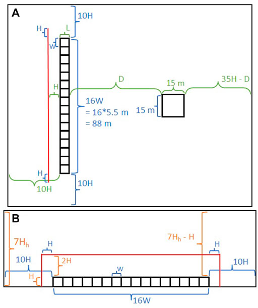
FIGURE 1. Schematic of the base case simulations where (A) is a top view and (B) is a front view looking along the flow into the vegetation fence. H: fence height (5.5 m), W: width of an individual tree (5.5 m), L: length of an individual tree (5.5 m), H_h: house height (9.1 m), D: distance between the house and the fence. The domain is 268 m long, 198 m wide, and 64 m tall. The red lines represent the outline of the firebrand injection region.

We chose the fence vegetation metrics to be representative of a row of 16 tightly-spaced medium-aged coast live oaks (Quercus agrifolia). The fence was 5.5 m tall, 88 m wide, and 5.5 m long. The fence was modeled as a porous region in the flow with a blocking coefficient of 5, representative of a dense vegetation canopy (Mueller, 2012).

The key dimensions in the domain were normalized by the vegetation height, H, and the height of the house, H_h. The computational domain extended more than 6 times the height of the nearest object in all directions to minimize boundary effects. The mesh resolution of 0.9 m was determined by the fence height, such that the fence was resolved by 6 cells per tree side.

Firebrands with a diameter of 1 mm were injected into the flow at a distance 1H upwind of the vegetation fence. The firebrands were uniformly distributed at 270 firebrands per m², in a region that extended from the ground to 2H above the vegetation fence and to 1H on both sides of the vegetation fence, for a total of 437,400 firebrands.

Sensitivity analysis experiments

We conducted a series of numerical experiments to investigate how various vegetation and firebrand metrics affected the flow and deposition dynamics compared to the base case simulations. We conducted an experiment for each level of the metrics shown in Table 1. Each experiment was conducted as described in the base case simulations except that the value of the metric under investigation was set to the specified level for that experiment and the house was located 16H downwind, just downwind of the flow reattachment point (described in the Flow simulations section). The house was located downwind of the reattachment point to investigate the best-case scenario for the fence by ensuring that the fence was not located in a region where we would expect enhanced deposition based on results from the base case experiments (described in the Flow simulations section). This would be analogous to planning for new construction a certain distance downwind of an existing mature stand of trees as planners can choose the location of new structures downwind of existing vegetation.

TABLE 1

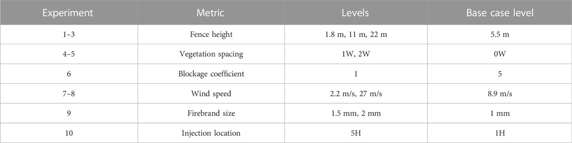
TABLE 1. Exploration of vegetation and firebrand metrics. H: height of the vegetation fence in the base case (5.5 m); W: width of an individual tree in the base case (5.5 m).

We chose the fence heights to represent various ages of Coast Live Oak (Quercus agrifolia): a young, newly planted tree with a height of 1.8 m, an older tree with a height of 11 m, and a mature tree with a height of 22 m. A height of 1.8 m is also representative of the size of many of the largest bushes found in the Los Angeles area, such as the California lilac (Ceanothus ‘Concha’). The number of trees was adjusted accordingly to maintain the base case fence width of 88 m; this resulted in 48 trees for the 1.8 m tall case, 8 trees for the 11 m tall case, and 4 trees for the 22 m tall case. We chose the vegetation spacing to investigate the effect of spacing between individual plants. The gaps represent one or two trees removed for every tree in the row. We chose the blockage coefficient to assess the performance of a fence with higher porosity. We chose the wind speeds to assess fence performance under light wind conditions vs. extreme Santa Ana wind events. We chose the firebrand sizes to investigate how the results would change for firebrands of slightly larger sizes. For short-to medium-range spotting, the largest firebrands tend to fall out quickly due to gravity, while firebrands on the small side of the size distribution may be transported far enough downwind to reach homes. We increased the distance between the injection location and the fence to assess the impact of the firebrand source location relative to the fence (and house) on deposition.

The domain configuration was the same as in the base case experiment for the 16H building location, except that the mesh resolution increased/decreased for shorter/taller fence heights such that the fence was always resolved in all directions by six grid cells; this resulted in mesh resolutions of 0.3 m, 1.8 m, and 3.7 m for the 1.8 m, 11 m, and 22 m tall fence cases, respectively. We set the domain extents such that the domain extended at least 6H upwind, on the sides, and above the tallest feature in the domain and 15H downwind of the largest object in the flow to avoid edge effects. The injection area, location, and quantity of firebrands were held constant for all cases except for the 5H injection location case, in which the injection was placed further upwind.

Results and discussion

Base case

Flow simulations

The simulated wind field for the flat terrain without any flow obstructions in the domain (no fence or house) was a horizontally homogeneous wind field with a vertical log profile and a wind speed of 8.9 m/s at a height of 6.1 m AGL (Supplementary Material). The time-averaged flow field simulated over the fence is shown in Figure 2. The fence induced several notable features into the flow field due to the mechanical effects of the fence on the flow (Figure 2). Some of the flow passed through the fence, but at a reduced rate, causing a pressure buildup upwind of the fence and forcing some flow up, over, and around the fence. This blocking effect caused a small region of reduced velocity immediately upwind of the fence that extended vertically from the ground to a short distance above the fence. A large wake region with reduced velocities formed, which extended far downwind of the fence. We defined the wake region throughout this study as the distance (downwind or vertically) required for the flow to return to within 10% of the unperturbed flow velocity. The wake region extended vertically from the ground to a height of approximately 2.5H and horizontally to 130H downwind of the fence. Twenty percent recovery was achieved at approximately 55H downwind. This was comparable to findings discussed in Counihan et al. (1974), which analyzed results from numerous experiments measuring flow over porous fencing. They reported that wake recovery varied as a function of porosity and ground roughness with distances of up to 30H required for 20% recovery downwind.

FIGURE 2

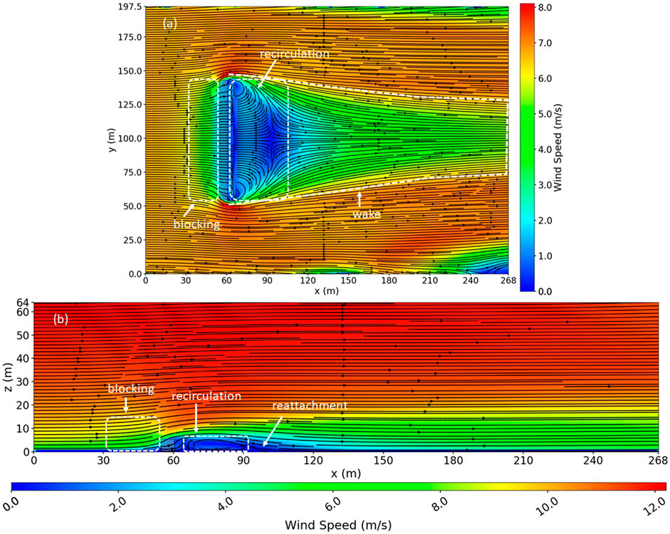
FIGURE 2. Simulated wind field over the vegetation fence without a house in the domain. (A) Top view slice at z = 1.4 m, which is the cell center of the second cell above the ground. (B) Side view slice down the middle of the domain. The dashed lines delineate various flow features induced by the fence, including a blocking region upwind of the fence, a wake region of reduced velocities extending far downwind of the fence, and a recirculation zone that forms due to flow separation behind the fence. The flow reattachment zone is also indicated.

The fence porosity was low enough (flow was sufficiently restricted) that flow was forced up and over the fence with enough momentum that it could not make the sharp corner on the lee side of the fence; instead, the flow separated from the fence, causing a recirculation region (an eddy) to form downwind of the fence. The recirculation region was characterized by a mean flow opposite in direction to the input wind. We quantified the size of the recirculation region by identifying cells with velocities with a negative x-component. The recirculation region was approximately 6H long and H deep. The flow reattached between approximately 6 and 10H downwind (Figure 2). The region downwind of the reattachment location was characterized by parallel streamlines. The wake characteristics, including the existence, location, and size of the recirculation zone, were a function of the vegetation porosity, size, and geometry and were expected to change as these vegetation metrics varied in the Sensitivity analysis section. The porosity and size affect the blocking effectiveness, while the shape and size of the vegetation determined whether the flow would separate (the “rounder” the vegetation, the more likely the flow is to stay attached).

The time-averaged flow field simulated around the house is shown in Figure 3. The house induced similar flow features as the fence, but with some important differences. Like the fence, a blocking region formed just upwind of the house, a larger wake region formed downwind of the house, and a recirculation zone formed immediately downwind of the house. Unlike the vegetation fence, the house acted as a complete obstruction to the flow, and all flow was forced over and around the house.

FIGURE 3

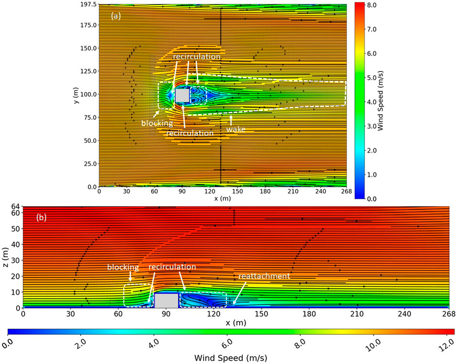
FIGURE 3. Simulated wind field over a house. (A) Top view slice at z = 1.4 m, which is the cell center of the second cell above the ground. (B) Side view slice down the middle of the domain, through the middle of the house. The dashed lines delineate various flow features induced by the house.

Several notable coherent structures are visible in the flow (Figure 3) and consistent with structures reported in previous investigations of flow around a wall-mounted cube (e.g., Martinuzzi and Topea, 1993; Shah and Ferziger, 1997; Paik et al., 2009). The house provided sufficient blockage to cause a small recirculation zone to form immediately upwind of the house close to the ground. Flow separation and recirculation upwind of the house occurred due to the formation of an adverse pressure gradient due to the flow blockage. This upwind flow separation was the origin of line vortices which advect downstream (Hunt et al., 1978) and was deflected around the sharp edges of the base of the house to form the well-known horseshoe vortex system (e.g., Martinuzzi and Topea, 1993). Evidence of a horseshoe vortex can be seen in Figure 3A. The enhanced blockage caused an increased speedup of the flow around the sides of the house compared to the fence. Small recirculation zones also formed on the sides of the house, causing a reversal of the mean flow along the sides of the house. Counter-rotating vortices formed in the immediate lee of the house due to periodic vortex shedding off the corners of the house. The wake region behind the house extended approximately 12H_h downwind.

The wake region that developed behind the house did not extend as high above the house as the wake region behind the fence extended vertically relative to the fence. The face area of the house was much smaller than that of the fence, as the fence was much longer than the house; thus, the flow was more easily routed around the house rather than being forced up and over. The wake of the house also recovered to the original approach profile much faster than for the vegetation fence, with the wake extending 1.5H_h in height and 27H_h downwind of the house.

Figures 4, 5 show the wind fields with the fence and house present in the flow and the house placed at various distances downwind of the fence. When the fence and house were both present, the flow features induced by each interacted in various ways, depending on their proximity. The development of the upwind stagnation point and the shear layer that develops along the sides of the house are strongly influenced by the flow impinging on the front face of the house (Martinuzzi and Havel, 2000). The flow impingement on the front face largely dictates the mechanical generation of flow features downwind as well as the characteristics of the blocking effects upwind (e.g., whether a stagnation point will form and the strength of the reversed flow if the flow separates).

FIGURE 4

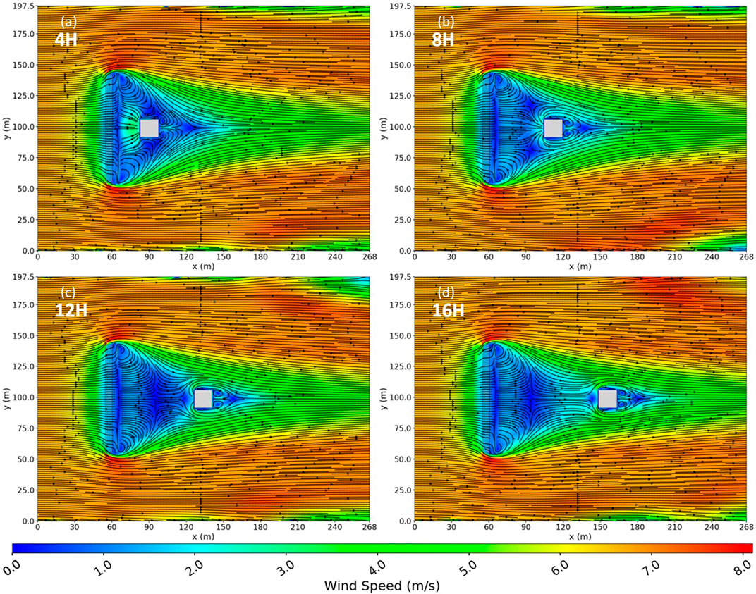
FIGURE 4. Top view slice at z = 1.4 m of the resulting wind fields with a vegetation fence and house included in the domain. The house is placed at various distances downwind of the vegetation fence in (A–D).

FIGURE 5

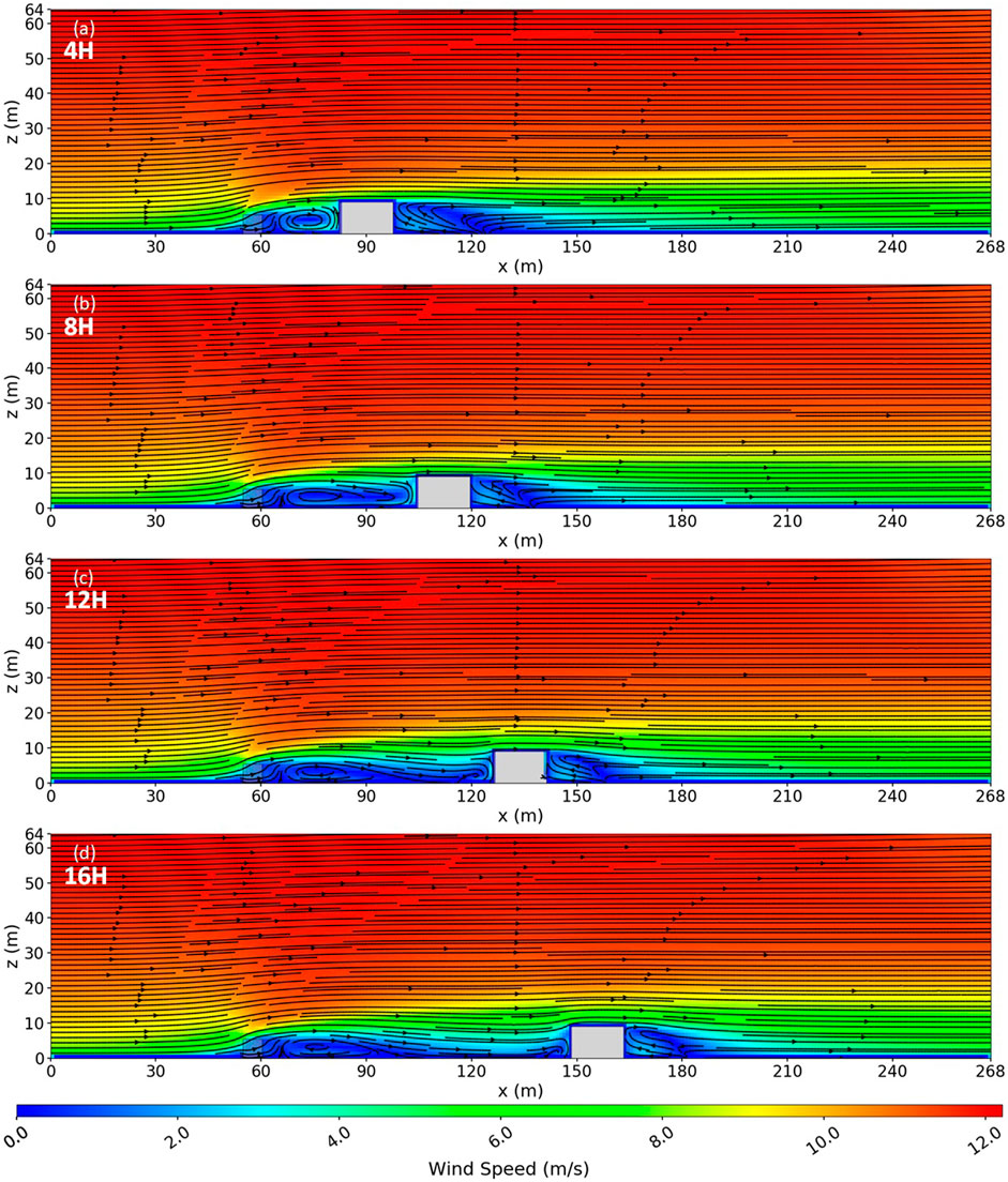
FIGURE 5. Side view slice along the middle of the domain of the simulated wind fields with a vegetation fence and house. The house is placed at various distances downwind of the vegetation fence in (A–D).

For the 4H case, the house was well within the turbulent recirculation zone of the vegetation fence. In this case, the recirculation region downwind of the fence was enhanced by the turbulent flow induced by the house (Figures 4A, 5A). For example, the strength of the reversed flow behind the fence increased by approximately 2 m/s. The house was also subject to higher levels of turbulence in the 4H and 8H cases due to its proximity to the recirculation region behind the fence. The Particle transport simulations section demonstrates the effect this has on firebrand deposition around the house. The interactions between the fence- and house-induced flow features diminished with increasing house distance downwind of the fence and were insignificant when the house was sufficiently downwind (∼15H) of the reattachment zone.

The house was still close to the reattachment zone in the 12H case and was still impacted by the fence-induced re-circulation zone (Figures 4C, 5C). The house was downwind of the reattachment zone for the 16H and 20H cases (Figures 4D, 5D; to save space, the 20H case is not shown as it was nearly identical to the 16H case). In these cases, the house was within the wake of the fence but was exposed to flow that had reattached to the surface and was trending back toward the unperturbed input wind condition. This flow was much less turbulent than that in the recirculation region behind the fence.

Particle transport simulations

When a firebrand is injected into the flow, it initially starts with the same velocity as the flow in the cell in which it was injected. As gravity acts on the firebrand, the firebrand begins a downward trajectory toward the ground. The trajectory becomes steeper with distance downwind due to decreased velocity as the firebrand nears the ground (i.e., a decreased ratio of the momentum force to the gravitational force acting on the firebrand). Simultaneously, the distance between individual firebrands increases with distance downwind due to turbulent diffusion. The horizontal distance an individual firebrand can travel depends on the firebrand position and velocity when it enters the flow (i.e., its injection location) and the wind velocity experienced by the firebrand at each height it passes along its trajectory through the flow.

The logarithmic wind profile of the unperturbed atmospheric boundary layer (ABL) is characterized by higher wind speeds aloft and lower wind speeds near the ground. The addition of the fence perturbs this logarithmic profile (Figures 4, 5), causing firebrands to experience different momentum forces in the perturbed flow and, thus, exhibit different trajectories compared to those in the unperturbed ABL. A firebrand transported over the fence above the wake region will have approximately the same trajectory as if the fence was not there. A firebrand that passes over or through the fence, but within the wake region, will experience a decreased momentum force exerted by the flow (due to the lower wind speeds in this region) and begin to drop sooner than it would without a fence. Firebrands that start close to the ground in the blocking region are deposited almost immediately.

The reversed flow in the recirculation region can transport firebrands back into the fence and cause deposition. When firebrands pass near or through the recirculation region, they can: continue around or over the recirculation region, enter it and escape, or enter it and become trapped. Firebrands enter the recirculation by passing in through the fence or descending into it downwind of the fence. Whether a firebrand is trapped within the recirculation region depends on the firebrand trajectory and momentum compared to that of the flow it encounters along its trajectory around or within the recirculation region. If the firebrand has enough momentum, it will continue nearly along its original trajectory. As the momentum of the flow begins to overtake that of the firebrand, the firebrand trajectory will become dominated by the flow. Firebrands without sufficient momentum will become trapped in the recirculation region if they enter it.

The firebrand deposition for each of the base case simulations is shown in Figure 6. When no house or fence was present (Figure 6aa), firebrands deposited almost uniformly in the y-direction for a given distance downwind with decreasing numbers of firebrands deposited per area with distance downwind. The band of deposition increased near the injection location due to the rapid deposition of firebrands injected near the ground.

FIGURE 6

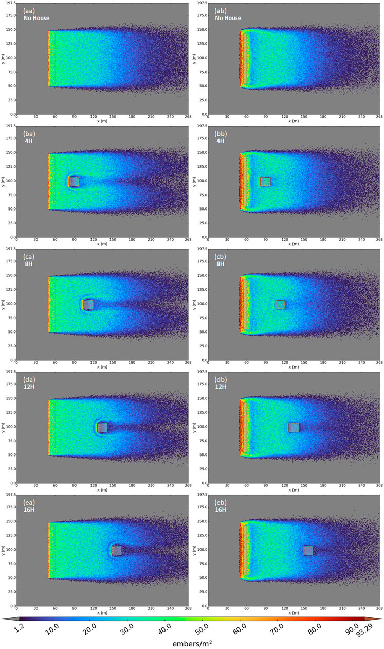
FIGURE 6. Firebrand deposition for the base case experiments. The house is located at various distances downwind with and without the fence present in the flow. The first letter (A–E) represents the distance downwind in the flow. The second letter represents the (A) absence or (B) presence of the fence. The colors represent the deposition per unit area.

When the fence was present in the flow with no house (Figure 6ab), regions of increased deposition formed just upwind of the fence and within the fence. A region of decreased deposition formed between the fence and the reattachment region. Deposition resumed as in the no-fence case just downwind of the reattachment zone. These results are similar to those for numerical flow simulations examining deposition behind a snow fence, which projected regions of increased deposition immediately upwind and downwind of an impervious fence and a region of decreased deposition within the recirculation zone (Liu et al., 2016). The reduced momentum in the blocking region upwind of the fence caused firebrands to deposit ahead of and within the fence (Figure 6ab). The reversed flow in the recirculation region transported firebrands back into the downwind side of the fence, leading to reduced deposition in this region and enhanced deposition in the immediate lee of the fence (Figure 6ab). The deposition increased again near the reattachment zone (Figure 6ab).

After adding a fence, deposition decreased on the front of the house in all cases and increased on the sides and the top of the house for the 4H, 8H, and 12H cases (Figures 6bb–db).

Table 2 shows the differences in deposition on the house between the fence and no-fence cases for a given house location downwind. The total deposition on the house increased for the 4H, 8H, and 12H cases compared to the no-fence case. This increase was largest for the 4H (34%) and 8H (33%) cases, in which the house was located within the recirculation region. The deposition increased by 10% increase for the 12H case. in which the house was located near the reattachment zone. The deposition on the house decreased for the 16H (−4.5%) and 20H (−11%) cases, with deposition decreasing with distance downwind. Also, fewer particles reached the house as the house moved farther downwind in the absence of a fence, with 10,532 and 2,913 particles reaching the house in the 4H and 20H cases, respectively (Table 2).

TABLE 2

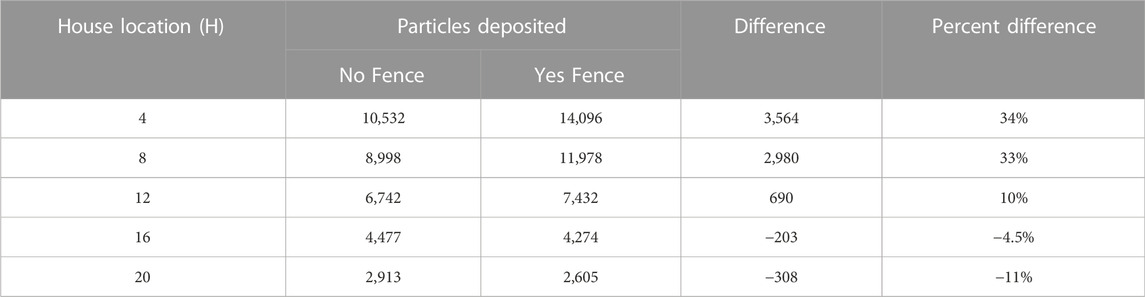
TABLE 2. Firebrand deposition totals and differences on the house with and without a vegetation fence at a given house location. Deposition on the house includes deposition on any surface of the house (i.e., all five exposed house surfaces). Positive numbers: increased total deposition; negative numbers: decreased total deposition.

These results indicated that the vegetation fence decreased firebrand deposition on the house when the house was located downwind of the reattachment zone. A distance of at least 15H was required to reduce deposition on the house for the vegetation fence configuration and firebrand characteristics investigated in the base case. The maximum reduction in deposition compared to the no-fence case was 11% and occurred for the 20H case.

Figure 7 shows deposition differences between the fence vs. no-fence cases along transects through the middle of the domain. To construct the transect plots, the domain is broken up into an x/y grid of bins. All particles landing within a given x/y grid region were counted for that bin. The calculations were performed with the house and ground together, meaning that regardless of z, the particles are counted for their bin grid (e.g., along the sides of the house the particles represent summed columns of values and are single z layers everywhere else). These results further confirmed the deposition patterns previously described in the vicinity of the fence. We observed a region of increased deposition just upwind of the fence, with a peak around x = 52 m that extended downwind through the fence to around x = 65 m (Figure 7). We also observed a region of decreased deposition extending from around x = 65 m to x = 75 m and a region of increased deposition (relative to the region within the recirculation zone) near the reattachment zone at around x = 75 m. Figure 7 also highlights the spatial patterns of deposition on and around the house. The deposition was decreased on the front of the house at all locations. We observed a pronounced increase in deposition on the top of the house for the 4H, 8H, and 12H cases and a small increase in deposition for 16H and 20H cases. Similarly, there was a pronounced increase in deposition on the sides of the house for the 4H, 8H, and 12H cases and a smaller but still notable increase in deposition for the 16H and 20H cases.

FIGURE 7

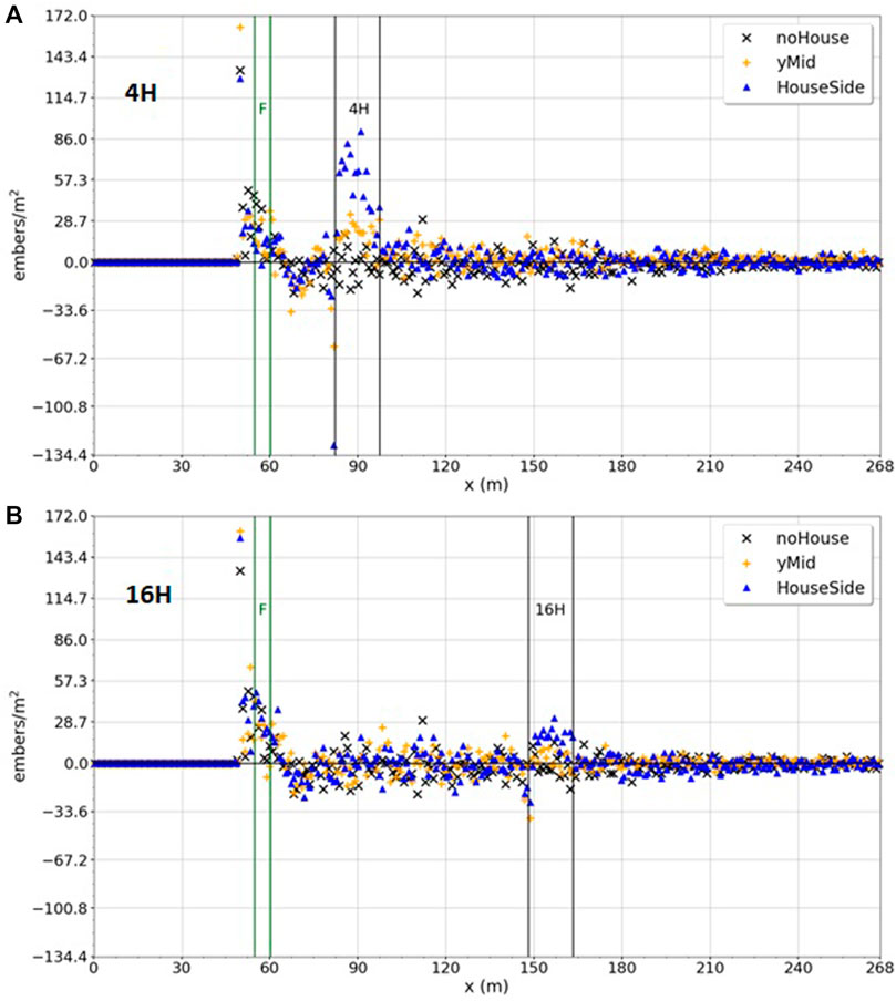
FIGURE 7. Differences in firebrand deposition with a fence vs. without along two transects down the middle of the domain for the base cases. The vertical lines near x = 60 m indicate the fence location. The vertical lines near 90 and 150 m indicate the house locations. Black ‘X’s: deposition along a transect running down the middle of the domain when no house is present. Gold ‘+’s: deposition along a transect running down the middle of the domain, through the centerline of the house. Blue triangles: deposition along a transect running along the side of the house. Positive numbers: increased deposition at a given location when a fence is present. Negative numbers: decreased deposition at a given location when a fence is present.

Ultimately, we observed decreased deposition on the front of the house and increased deposition on the sides and top of the house for all cases. The increased deposition on the top of the house was likely due to the region of decreased wind speeds just downwind of the vegetation fence that extended vertically above the house. Firebrands that used to pass through that region at a higher wind speed and over the house with no fence present now passed through the region of reduced wind speeds that extended above the house caused by the fence and fell out sooner. Therefore, vegetation fences can also increase deposition on the house by allowing firebrands aloft to descend more quickly due to reduced flow momentum over the house. The increased deposition on the sides likely occurred due to interactions between the fence and house wakes. As discussed in the Flow simulations section, the wake that formed around the house was driven by the flow that impacted the front of the house. The proximity of the fence and the wake that formed behind it determined the flow characteristics impacting the house. Ultimately, the deposition patterns on and around the house were a function of the house geometry and the flow characteristics (e.g., shear profile and turbulence structure) impacting it. Future work is warranted to examine these complex flow interactions and mechanisms governing particle deposition.

Sensitivity analysis

Fence height

Figures 8, 9 show the wind field for various fence height cases with both the fence and the house present in the flow. For the 1.8 m fence height case, the fence was 7.3 m shorter than the house and affected only a shallow layer of approach flow to the house (Figure 9A). The size of the recirculation region that formed behind the fence was approximately 2.6H long and 0.5H deep. The wake extended to approximately 40H downwind and 2H vertically (not shown). In this case, the house had a larger effect on the flow field compared to the fence (Figures 8A, 9A). The recirculation regions that formed upwind and downwind of the house were larger in the x- and z-dimensions than that formed behind the fence (Figures 8A, 9A).

FIGURE 8

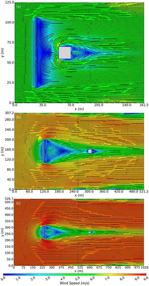
FIGURE 8. Top view slice at z = 0.46 m of the simulated wind fields for various fence heights with both fence and house present in the flow. Fence heights of (A) 1.8 m, (B) 11 m, and (C) 22 m.

FIGURE 9

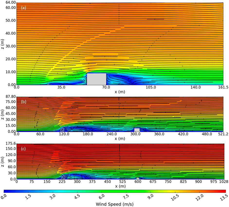
FIGURE 9. Side view slice down the middle of the domain of the simulated wind fields for various fence heights with both the fence and house present in the flow. Fence heights of (A) 1.8 m, (B) 11 m, and (C) 22 m.

For the 11 and 22 m fence height cases, the fence was 1.8 m and 13 m taller than the house, respectively. As expected, the length and depth of the recirculation zones scaled with the height of the fence, but with slightly different scaling than in the previous cases (6H long and 0.7H deep for the 11 m case and 5H long and 0.7H deep for the 22 m case). As the fence height increased, the house (located at 16H downwind of the fence) was located in the region where the wake was beginning to narrow in the y-dimension (Figures 8B,C). The depth of the wake was roughly 2.5H for all cases, which was the same as in the base case.

The deposition patterns for the 1.8 m case were like those in the base case, with increased deposition upwind of the fence, within the fence, and immediately downwind of the fence and a narrow (due to the short fence height) band of decreased deposition upwind of the reattachment zone. We observed enhanced deposition along the front of the house as in the base case experiments. The total deposition on the house increased by 16% compared to the no-fence case (Table 3), likely due to interactions of the wake region of the fence with the upwind recirculation region of the house. A very strong recirculation region formed upwind of the house, with reversed flow around 5 m/s (Figures 8A, 9A). The top of the house was exposed to higher speeds than in the base case because the fence was much shorter than the house, which allowed unperturbed flow to reach the top of the house. The base of the house, however, was impacted by the wake region of the fence-perturbed flow. The increased shear likely allowed for the formation of a more intense recirculation upwind of the house and, thus, more deposition in this location compared to the no-fence case.

TABLE 3

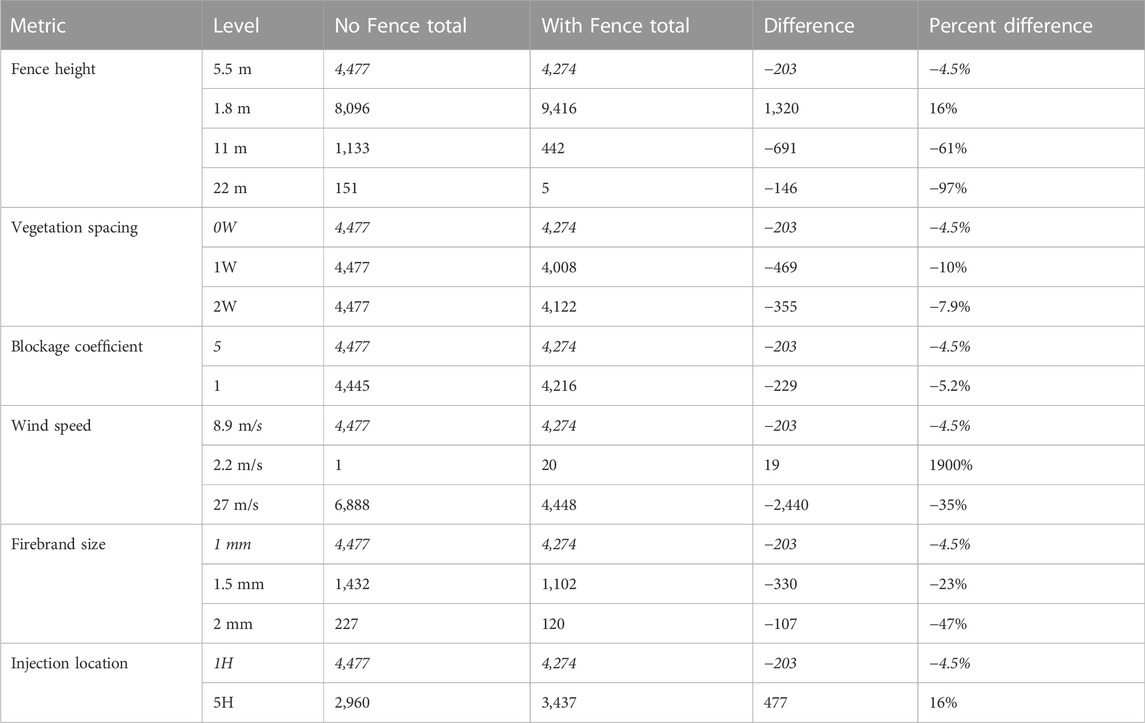
TABLE 3. Deposition totals and differences on the house for the sensitivity analysis cases. Positive numbers: increased total deposition compared to the no-fence case; negative numbers: decreased total deposition compared to the no-fence case; italics: base case values.

As the house distance from the firebrand source increased, the total number of particles reaching the house decreased sharply, with only 1,133 particles and 151 particles reaching the house for the no-fence 11 m and 22 m cases, respectively, compared to 8,096 particles for the no-fence 1.8 m case. The inclusion of the fence in these simulations resulted in 61% and 97% decreases in deposition on the house for the 11 m and 22 m fence cases, respectively. While these percent reductions were large, the total number of particles reaching the house without the fence was small, particularly for the 22 m case. Taller fences require the house to be much farther downwind to be sufficiently far downwind of the reattachment zone. For these taller fence heights, the recirculation region became sufficiently deep such that relocating the fence to put the house within the recirculation region could be effective. This option could be explored in future work.

The firebrand injection depth was shorter than the fence for the 11 m (injection depth ∼2/3H) and 22 m (injection depth ∼½ H) cases, which likely increased the effectiveness of the fence compared to the base case. The fence has the largest impact on flow and deposition in the shallow layer affected by the fence (roughly 2.5H). Particles injected above this height are largely unaffected by the fence and can still impact the house as they travel with the mean wind and descend due to gravity. When these same cases were repeated using an injection that scaled with height (not shown), the resulting deposition was similar to that of the base case with decreased deposition on the house by 23% for the 11 m case and 10% for the 22 m case, which is an improvement from the base case, but much less effective compared to the same cases with firebrands released at the lower heights (Table 3).

Vegetation spacing

Figure 10 shows the wind field for the 1W gap vegetation spacing case with both the fence and the house present in the flow. The gaps were created by removing alternating trees in the fence. The blocking region upwind of the fence was roughly the same size as that in the base case. The flow increased as it passed through the gaps and decreased as it passed through the porous vegetation structures, forming small individual recirculation zones just downwind of each of the individual fence sections. These recirculation zones were much smaller than the original single large recirculation zone in the base case. In addition, the fence wake region of the 1W gap was smaller in size than that in the base case. The wake did not affect the flow around the house as much as it did in the base case. In particular, the fence wake no longer extended as high above the house (Figure 10).

FIGURE 10

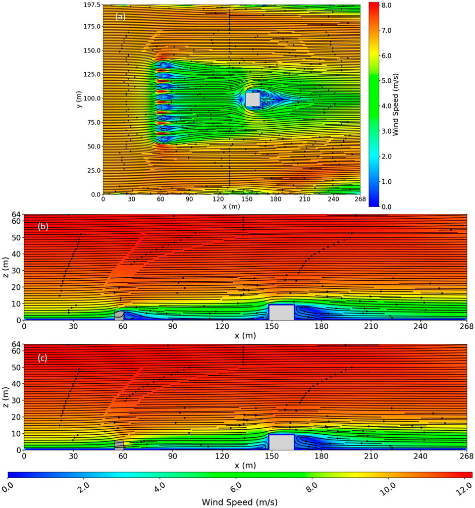
FIGURE 10. Simulated wind field for 1W gap vegetation spacing with both fence and house present in the flow. (A) Top view slice at z = 1.4 m, which is the cell center of the second cell above the ground. (B) Side view slice down the middle of the tree just to the left of the middle gap at y = 102 m, just to the left of the center of the house. (C) Side view slice down the middle of the middle gap at y = 96 m.

Figure 11 shows the wind field for the 2W gap vegetation spacing case with both the fence and the house present in the flow. The flow was like the 1W gap vegetation spacing case, with a wider speedup region between each gap and bands of slightly higher wind speeds in the wake region, just downwind of the gaps. The recirculation regions behind the remaining sections of vegetation in the fence for the 2W gap case were similar in size to those of the 1W gap case. The blocking region upwind of the fence was smaller for the 2W gap case compared to the 1W gap case. The blocking region extended a shorter distance upwind and was slightly shorter in the z-direction for the 2W gap case compared to the 1W gap case. The fence wake in the 2W gap case was similar in size to the 1W gap case and no longer extended as high above the house as it did in the base case.

FIGURE 11

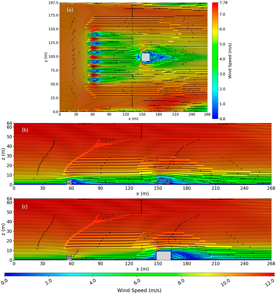
FIGURE 11. Simulated wind field for 2W gap vegetation spacing with both fence and house present in the flow. (A) Top view slice at z = 1.4 m, which is the cell center of the second cell above the ground. (B) Side view slice down the middle of the tree just to the left of the middle gap at y = 107 m, just to the left of the house. (C) Side view slice down the middle of the middle gap at y = 99 m, down the center of the domain, and down the center of the house, still within the region of the house.

Figure 12 shows the firebrand deposition for the 1W gap vegetation spacing case. We observed bands of increased deposition downwind of the fence gaps where higher-momentum flow was able to pass through. The deposition upwind of the fence was like that in the base case. The deposition pattern on the downwind side of the fence differed from the base case, with an area of decreased deposition immediately downwind of the fence compared to increased deposition in the base case. The increased deposition within the fence suggested that firebrands transported by the reversed flow downwind of the fence traveled back into and were deposited within the fence instead of accumulating at the downwind edge. Other than the increased deposition downwind of the fence gaps and additional deposition within the vegetation fence, the deposition pattern for the 1W case was like that of the base case. The total deposition on the house showed a small decrease for the 1W gap case (−10%) compared to the base case (−4.5%) (Table 3).

FIGURE 12

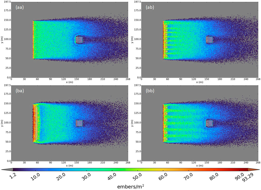
FIGURE 12. Firebrand deposition for 1W and 2W gap vegetation spacing. (aa) 1W gap without the fence. (ab,bb) 1W and 2W gaps with the fence, respectively. (ba) Repeat of Figure 6eb for easier comparison showing that the base case results for 1W and 2W gaps without a fence are the same.

The deposition for the 2W gap case (created by removing two trees between each remaining tree in the fence) was similar to that of the 1W gap case, except that the decreased deposition regions immediately downwind of the filled sections of the fence extended out to the sides into the banded regions of regular deposition immediately downwind of the gaps (Figure 12).

Table 3 shows the firebrand deposition totals for the 1W and 2W gap cases vs. the base case. Both the 1W and 2W gap cases showed decreased deposition compared to the base case. However, the 2W case showed slightly more deposition compared to the 1W case, suggesting a threshold for which vegetation spacing increased effectiveness. This could also be caused by the gaps lining up differently with the house. These potential explanations require exploration in future work.

Blockage coefficient

Decreasing the blockage coefficient from 5 to 1 did not appreciably change the flow or deposition from the base case. The only notable difference was the size and shape of the downwind recirculation region; it was slightly shorter in height (0.2H) and length compared to the base case and was shorter in the x-dimension along the center of the fence (0.5H long) and longer in the x-dimension near the edges of the fence (2H long). The size and shape of the wake region were like those of the base case. The deposition pattern was nearly identical to that in the base case, although the deposition region just downwind of the fence extended slightly further downwind. The deposition behind the fence appeared to extend less distance downwind as it curved in behind the edges of the fence. The deposition on the house for the blockage coefficient 1 case did not differ substantially from the base case (Table 3), suggesting that the vegetation effective blockage could decrease somewhat without compromising effectiveness.

Wind speed

The wind fields for the 2.2 m/s and 27 m/s wind speed cases were like those in the base case. The blocking regions, wake regions, and recirculation zones all had the same size and shape as those in the base case. The only notable difference from the base case was that the magnitude of the velocities decreased for the 2.2 m/s case and increased for the 27 m/s case. This result was anticipated, as the size and shape of the flow obstruction determine the wake structure for flows with Reynold’s numbers (Re) typical of the ABL (e.g., Martinuzzi and Havel, 2000; Meinders and Hanjalic, 2002; Paik et al., 2009).

Figure 13 shows the firebrand deposition for these cases. In the 2.2 m/s case, the firebrands fell out much sooner than in the base case and most did not reach the house, even without the fence. We observed increased deposition upwind of the fence compared to the base case. No region of increased deposition just behind the fence occurred, unlike in the base case. Table 3 shows the firebrand deposition totals for the 2.2 m/s wind speed case vs. the base case. Essentially no particles made it to the house and so, although the percent difference was large, it was not meaningful. The 2.2 m/s wind speed was not strong enough to carry the particles to the house before they settled out due to gravity.

FIGURE 13

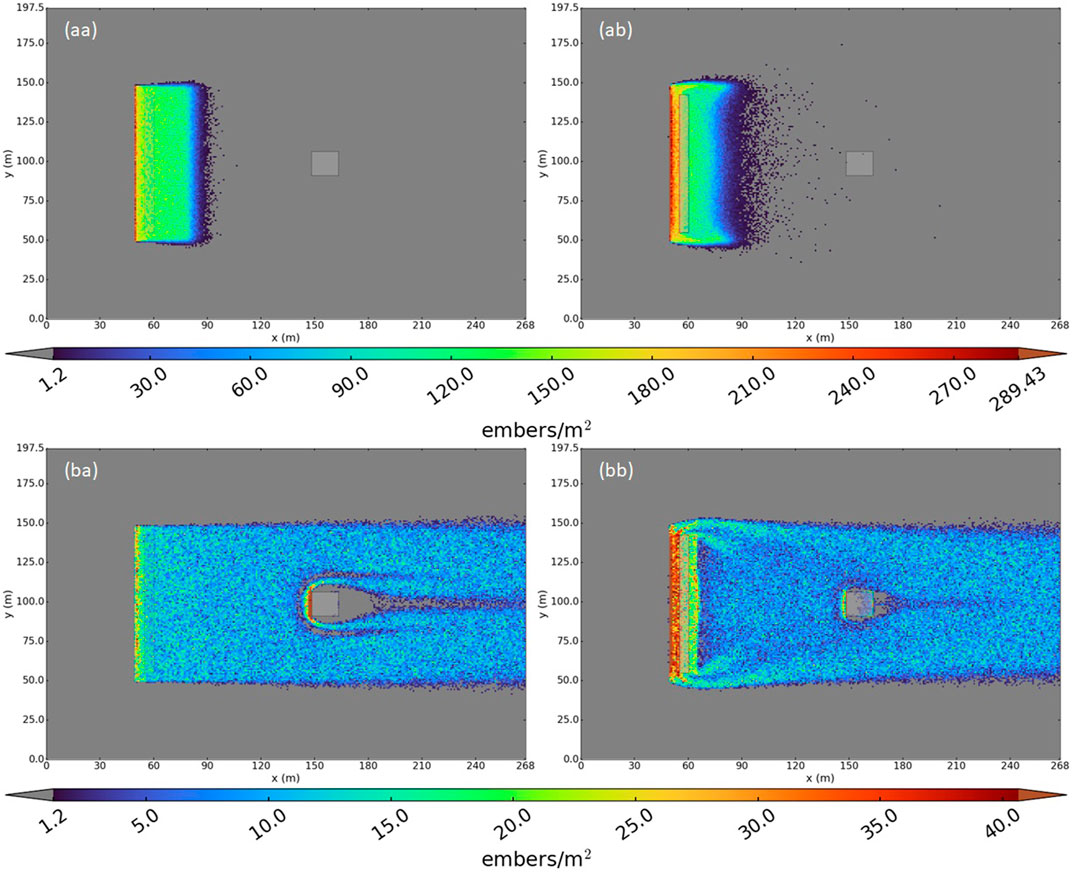
FIGURE 13. Firebrand deposition for the 2.2 m/s and 27 m/s wind speed cases. (aa) 2.2 m/s without the fence. (ab) 2.2 m/s with the fence. (ba) 27 m/s without the fence. (bb) 27 m/s with the fence. Colors: deposition per unit area.

The deposition patterns for the 27 m/s case were like those in the base case. Without the fence, enhanced deposition occurred on the front of the house and reduced deposition on the top and sides of the house, on the ground to the sides of the house, and downwind of the house due to the flow effects induced by the house (blocking region in front and wake region behind the house). The number of firebrands that deposited on the front of the house decreased when the fence was added; however, the deposition increased along the top and sides of the house. The deposition on the house decreased by 35% when the fence was present, primarily due to reduced deposition on the front of the house. While this was a substantial reduction in deposition compared to the base case (−35% vs. −4.5%), the total number of particles deposited on the house was similar (4448 vs. 4274 particles). Figure 13 also shows that most of the decrease in deposition for the 27 m/s case was due to decreased deposition on the front of the house, with increased deposition along the top and sides of the house when the fence was present.

Firebrand size

As expected, the 1.5 mm and 2 mm firebrands did not travel as far as the 1 mm firebrands in the base case. The firebrands barely reached the house without the fence in the flow. The deposition patterns were like those in the base case, but with increased deposition upwind of the house due to the larger firebrands settling out faster due to gravity. The few firebrands that reached the house in these cases impacted the house with steeper trajectories as they descended from the highest layers of the firebrand source region.

Injection location

The 5H injection location deposition was like that of the base case (Figure 14). We observed a slight increase in deposition upwind of the fence to a short distance downwind of the fence and a large region of decreased deposition downwind of the vegetation fence in the wake region. In contrast to the base case, we observed increased deposition on the front of the house. Overall, the fence enhanced deposition when the injection location moved upwind, likely due to firebrands from higher aloft descending toward the house along steeper trajectories. The particle trajectories and the effects of particle size should be further explored in future work.

FIGURE 14

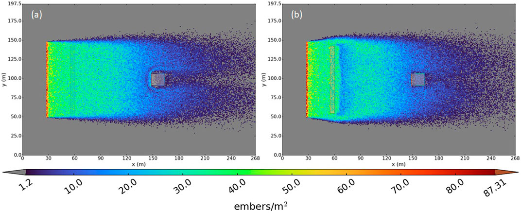
FIGURE 14. Firebrand deposition for the 5H injection location case. (A) Without the fence. (B) With the fence.

Limitations and future work

One key assumption in this study was that a vegetation fence could trap firebrands without igniting. If the fence ignited, it could become a source of firebrands nearer to the house. The fence would also become less effective as a flow barrier once the vegetation is consumed and less of the flow is blocked. Vegetation used as the fence material should be a fire-resistant species. Routine maintenance would likely also be necessary for irrigation and clean-up of litter material deposited by the vegetation. It is not clear whether these requirements could practically be met; if so, these findings would be of substantial interest to new construction planners and landscape architects in fire-prone regions. These study findings are also relevant for other types of porous fences and could be used to guide the design of non-vegetated fencing options.

There are some uncertainties associated with the flow and particle models. For instance, additional turbulence models could be considered in future work. Some research suggests that the RNG k-epsilon turbulence model better resolves flow in the outer regions of the horseshoe vortex as it wraps around an obstacle, which could be an important consideration for particle transport near the house. Physically based correlations giving a probability for whether a particle will stick as it passes through the vegetation fence and stick or rebound when it contacts a wall could also be investigated.

The effects of firebrand particle shape and density require further investigation. We assumed that the particles were inert and spherical with the density of charred wood. Firebrand transport is strongly linked to the particle properties and while the properties used in this work are representative of some firebrands, testing of other representative particle configurations is warranted to determine the sensitivity of these results to these particle metrics.

This study focused on short-to medium-range spotting. Thus, the source term was configured to be representative of firebrands generated nearby entering the domain. The source term was a shallow layer (on the order of the fence height) of inert particles with constant density and size. The representativeness of this source term could be evaluated in future work. The effects of the injection angle and injection velocity of the particles could also be investigated. A brief analysis of different injection angles and velocities in the IBHS experiments showed some sensitivity of the deposition pattern to these initial particle conditions (Supplementary Material). A porous fence, as described in this work, would not be expected to affect impingement from long-range firebrand spotting as firebrands raining down on the house from long-range spotting would not travel through the near-surface flow affected by the fence.

Deposition patterns in the immediate vicinity of the house are determined by the house geometry and flow characteristics (e.g., shear profile, turbulence structure, etc.) that impact the house. A deeper investigation of shear and turbulence dynamics in the vicinity of houses with various geometries could improve the understanding of interactions between the flow features induced by the fence and the house. Future work is warranted to examine these complex flow interactions and the mechanisms governing particle deposition.

Future work could also investigate additional fence configurations, including repeated rows of fencing, varied fence length and height; more sophisticated vegetation representation, and additional wind directions with respect to the fence.

Conclusion

This study investigated the effectiveness of a porous fence for inducing firebrand deposition upwind of and reducing firebrand impingement on homes from short-to medium-range spotting. We investigated house location in proximity to the fence along with several properties of the fence, flow, and firebrands including fence height (1.8–22 m), fence porosity, vegetation spacing (1W–2W), wind speed (2.2–27 m/s), firebrand source location (1H–5H upwind), and firebrand particle size (1–2 mm). Some of the key findings from this work include:

• A porous fence decreased the deposition on a house by up to 35% as long as the house was located sufficiently downwind of the flow reattachment zone (roughly 15H downwind of the fence).

• A fence only affected the flow and offered protection for a shallow layer above the ground. The depth of this layer was on the order of the height of the fence.

• A fence increased the deposition on a house if the house was located too close to the fence (within ∼15H) or if the house was substantially taller than the fence (e.g., 1.8 m fence height case).

• The fence should be tall enough that the depth of the wake region that forms behind the fence is on the order of the height of the house or taller.

• The location of the firebrand source relative to the house was the most important metric determining whether firebrands would reach and deposit on a house. The number of firebrands reaching the house was reduced by 36% when the distance from the source was increased by a factor of 3 (4H–12H) and by 72% when the distance was increased by a factor of 5 (4H–20H).

• Increased fence height offered protection up to a greater height but also caused the recirculation zone to grow in length downwind, requiring greater distances between the fence and the house.

• Vegetation spacing on the order of the size of the vegetation (1–2W) can increase the fence effectiveness (10% vs. 4.5% reduction at 15H for the 1W vs. 0W spacings, respectively).

• A slightly more porous fence can offer similar protection to a less porous fence, although there is likely a porosity threshold.

• Fences were most effective at reducing firebrand deposition on homes under high winds (35% vs. 4.5% reduction at 15H for the 27 m/s vs. 8.9 m/s case). However, firebrands also travel further under high winds, thus increasing the risk of firebrands reaching a home.

• The size and shape of the wake and recirculation region did not change with wind speed. The wake characteristics were determined as a function of the geometry and porosity of the flow obstructions under the types of ABL flows examined here.

• As particle size increases, the transport distance rapidly decreases, with a 95% reduction in particles reaching the house when the particle size increased from 1 mm to 2 mm.

• Particles falling on a steeper trajectory have more momentum and are less likely to be impacted by the wake region flow. If firebrands fall from a long enough distance before reaching the shallow flow region altered by the fence (e.g., the 5H injection case), they may be less affected by the wake region of the fence, potentially decreasing the protection provided by the fence.

With firebrand impingement on homes a leading cause of home ignitions, every step a homeowner can take to minimize that risk is important. In some communities, the addition of some type of porous fencing may offer additional protection from nearby firebrand sources, particularly during high wind events, and is worth additional investigation. However, fencing can also increase deposition in some cases. The findings of this study highlight the importance of maximizing the distance between potential firebrand sources and homes.

Data availability statement

Source code used for numerical simulations can be found at https://github.com/firelab/canopy-wake.

Author contributions

NW conceived the study. LA developed the code and performed the numerical simulations. LA analyzed and interpreted the results under the supervision of NW. LA and NW wrote and edited the manuscript.

Funding

This work was funded by the Resource Conservation District of the Santa Monica Mountains and the United States Department of Agriculture Forest Service Rocky Mountain Research Station.

Acknowledgments

We thank Dr. David Blunck and Dr. Bret Butler for reviewing an early draft of this manuscript. We thank Dr. Jack Cohen for discussions regarding the feasibility of using fences for protecting homes from ember impingement. Thanks to three reviewers whose comments greatly improved the readability of the paper.

Conflict of interest

The authors declare that the research was conducted in the absence of any commercial or financial relationships that could be construed as a potential conflict of interest.

Publisher’s note

All claims expressed in this article are solely those of the authors and do not necessarily represent those of their affiliated organizations, or those of the publisher, the editors, and the reviewers. Any product that may be evaluated in this article, or claim that may be made by its manufacturer, is not guaranteed or endorsed by the publisher.

Supplementary material

The Supplementary Material for this article can be found online at: https://www.frontiersin.org/articles/10.3389/fmech.2022.1059018/full#supplementary-material

References

Adusumilli, S., Chaplen, J. E., and Blunck, D. L. (2021). Firebrand generation rates at the source for trees and a shrub. Front. Mech. Eng. 7. 35. doi:10.3389/fmech.2021.655593

CrossRef Full Text | Google Scholar

Bailey, B. N. (2017). Numerical considerations for Lagrangian stochastic dispersion models: Eliminating rogue trajectories, and the importance of numerical accuracy. Bound. Layer. Meteorol. 162 (1), 43–70. doi:10.1007/s10546-016-0181-6

CrossRef Full Text | Google Scholar

Bitog, J. P., Lee, I B., Hwang, H S., Shin, M H., Hong, S W., and Seo, I H. (2012). Numerical simulation study of a tree windbreak. Biosyst. Eng. 111, 40–48. doi:10.1016/j.biosystemseng.2011.10.006

CrossRef Full Text | Google Scholar

CAL FIRE (California Department of Forestry and Fire Protection), (2022). Defensible space. CAL FIRE website. https://www.fire.ca.gov/programs/communications/defensible-space-prc-4291/ (Accessed November 9, 2022).

Google Scholar

Cohen, J. D. (2000). Preventing disaster: Home ignitability in the wildland-urban interface. J. For. 98 (3), 15–21. doi:10.1093/jof/98.3.15

CrossRef Full Text | Google Scholar

Cohen, J. D., and Stratton, R. D. (2008). Home destruction evaluation: Grass valley fire. Lake arrowhead, California. Vallejo, CA, USA: US Department of Agriculture, Forest Service, 26. Technical Paper R5-TP-026b.

Google Scholar

Counihan, J., Hunt, J. C. R., and Jackson, P. S. (1974). Wakes behind two-dimensional surface obstacles in turbulent boundary layers. J. Fluid Mech. 64 (3), 529–564. doi:10.1017/s0022112074002539

CrossRef Full Text | Google Scholar

Dalpé, B., and Masson, C. (2009). Numerical simulation of wind flow near a forest edge. J. Wind Eng. Industrial Aerodynamics 97 (5–6), 228–241. doi:10.1016/j.jweia.2009.06.008

CrossRef Full Text | Google Scholar

Du, S., Petrie, J., and Shi, X. (2017) Use of snow fences to reduce the impacts of snowdrifts on highways: Renewed perspective. Transp. Res. Rec. J. Transp. Res. Board. 2613. National Research Council, 45–51. doi:10.3141/2613-06

CrossRef Full Text | Google Scholar

Gao, Z., Bresson, R., Qu, Y., Milliez, M., de Munck, C., and Carissimo, B. (2018). High resolution unsteady RANS simulation of wind, thermal effects and pollution dispersion for studying urban renewal scenarios in a neighborhood of Toulouse. Urban Clim. 23, 114–130. doi:10.1016/j.uclim.2016.11.002

CrossRef Full Text | Google Scholar

Harris, H. (2011) Analysis and parameterization of the flight of firebrand generation experiments. Masters thesis. Clemson University. Sikes Hall, SC, USA. https://tigerprints.clemson.edu/all_theses.

Google Scholar

Hudson, T. R., Bray, R. B., Blunck, D. L., Page, W., and Butler, B. (2020). Effects of fuel morphology on ember generation characteristics at the tree scale. Int. J. Wildland Fire 29 (11), 1042–1051. doi:10.1071/WF19182

CrossRef Full Text | Google Scholar

Hunt, J. C. R., Abell, C. J., Peterka, J. A., and Woo, H. (1978). Kinematical studies of the flows around free or surface-mounted obstacles; applying topology to flow visualization. J. Fluid Mech. 86, 179–200. doi:10.1017/s0022112078001068

CrossRef Full Text | Google Scholar

Liu, D., Li, Y., Wang, B., Hu, P., and Zhang, J. (2016). Mechanism and effects of snow accumulations and controls by lightweight snow fences. J. Mod. Transp. 24 (4), 261–269. doi:10.1007/s40534-016-0115-5

CrossRef Full Text | Google Scholar

Los Angeles County, (2019). After action review of the Woolsey fire incident. http://file.lacounty.gov/SDSInter/bos/supdocs/144968.pdf (accessed September 30, 2022).

Google Scholar

Maranghides, A., and Mell, W. (2011). A case study of a community affected by the Witch and Guejito wildland fires. Fire Technol. 47 (2), 379–420. doi:10.1007/s10694-010-0164-y

CrossRef Full Text | Google Scholar

Martinuzzi, R. J., and Havel, B. (2000). Turbulent flow around two interfering surface-mounted cubic obstacles in tandem arrangement. J. Fluids Eng. 122 (1), 24-31. doi:10.1115/1.483222

CrossRef Full Text | Google Scholar

Martinuzzi, R. R., and Topea, C. (1993). The flow around surface-mounted, prismatic obstacles placed in a fully developed channel flow (data bank contribution). J. Fluids Eng. 115 (85), 85–92. doi:10.1115/1.2910118

CrossRef Full Text | Google Scholar

Meinders, E. R., and Hanjalic, K. (2002). Experimental study of the convective heat transfer from in-line and staggered configurations of two wall-mounted cubes. Int. J. Heat Mass Transf. 45, 465–482. doi:10.1016/s0017-9310(01)00180-6

CrossRef Full Text | Google Scholar

Mueller, E. V. (2012) LES modeling of flow through vegetation with applications to wildland fires. Masters thesis. Worcester Polytechnic Institute. Worcester, MA, USA. https://digitalcommons.wpi.edu/etd-theses/334.

Google Scholar

Nader, G., Nakamura, G., de Lasaux, M., Quarles, S., and Valachovic, Y. (2007). Home landscaping for fire. Oakland, CA: ANR Publication, 8228. http://anrcatalog.ucdavis.edu.

Google Scholar

Paik, J., Sotiropoulos, F., and Porte-Agel, F. (2009). Detached eddy simulation of flow around two wall-mounted cubes in tandem. Int. J. Heat Fluid Flow 30, 286–305. doi:10.1016/j.ijheatfluidflow.2009.01.006

CrossRef Full Text | Google Scholar

RCDSMM (Resource conservation District of the Santa Monica mountains), (2022). Sustainable defensible space. https://defensiblespace.org/landscape/landscape-new/(Accessed on November 9, 2022).

Google Scholar

Richards, P. J., and Norris, S. E. (2011). Appropriate boundary conditions for computational wind engineering models revisited. J. Wind Eng. Industrial Aerodynamics 99 (4), 257–266. doi:10.1016/j.jweia.2010.12.008

CrossRef Full Text | Google Scholar

Richter, F., Atreya, A., Kotsovinos, P., and Rein, G. (2019). The effect of chemical composition on the charring of wood across scales. Proc. Combust. Inst. 37 (3), 4053–4061. doi:10.1016/j.proci.2018.06.080

CrossRef Full Text | Google Scholar

Salim, M. H., Schlunzen, K. H., and Grawe, D. (2015). Including trees in the numerical simulations of the wind flow in urban areas: Should we care? J. Wind Eng. Industrial Aerodynamics 144, 84–95. doi:10.1016/j.jweia.2015.05.004

CrossRef Full Text | Google Scholar

Segersson, D. (2017). “A tutorial to urban wind flow using OpenFOAM,” in Proceedings of CFD with OpenSource software. Editor Nilsson.H. doi Stockholm: Stockholm University and Swedish Meteorological and Hydrological Institute. doi:10.17196/OS_CFD#YEAR_2017

CrossRef Full Text | Google Scholar

Shah, K. B., and Ferziger, J. H. (1997). A fluid mechanicians view of wind engineering: Large eddy simulation of flow past a cubic obstacle. J. Wind Eng. Industrial Aerodynamics 67-68, 211–224. doi:10.1016/s0167-6105(97)00074-3

CrossRef Full Text | Google Scholar

Taylor, A. (2018) Photos: The Woolsey fire leaves devastation in malibu, California. https://www.theatlantic.com/photo/2018/11/photos-woolsey-fire-leaves-devastation-malibu-california/575578/ (Accessed September 30, 2018). The atlantic, 11 nov.

Google Scholar

Tong, Z., Baldauf, R. W., Isakov, V., Deshmukh, P., and Max Zhang, K. (2016). Roadside vegetation barrier designs to mitigate near-road air pollution impacts. Sci. Total Environ. 541, 920–927. doi:10.1016/j.scitotenv.2015.09.067

PubMed Abstract | CrossRef Full Text | Google Scholar

Wagenbrenner, N. S., Forthofer, J. M., Page, W. G., and Butler, B. W. (2019). Development and evaluation of a Reynolds-averaged Navier-Stokes solver in WindNinja for operational wildland fire applications. Atmosphere 10 (11), 672. doi:10.3390/atmos10110672

CrossRef Full Text | Google Scholar

Weller, H. G., Tabor, G., Jasak, H., and Fureby, C. (1998). A tensorial approach to computational continuum mechanics using object-oriented techniques. Comput. Phys. 12, 620. doi:10.1063/1.168744

CrossRef Full Text | Google Scholar

Nomenclature

ABL atmospheric boundary layer

AGL above ground level [m]

$a_{p,i}$ acceleration of a given particle $p$ for component direction $i$ [m/s²]

$b$ blockage coefficient [1/m]

BC boundary conditions

${\beta }_d$ turbulence constant for porous media flows [unitless]

${\beta }_p$ turbulence constant for porous media flows [unitless]

$C_d$ drag coefficient [unitless]

$C_{\epsilon 1}$ turbulence constant [unitless]

$C_{\epsilon 2}$ turbulence constant [unitless]

$C_{\epsilon 4}$ turbulence constant for porous media flows [unitless]

$C_{\epsilon 5}$ turbulence constant for porous media flows [unitless]

$C_{\mu }$ turbulence constant [unitless]

$C_0$ universal constant for Lagrangian particle modeling [unitless]

D distance between the house and the fence, x component direction [m]

$d_p$ diameter of a given particle $p$ [mm]

$\mathrm{d}\mathrm{t}$ timestep [s]

$d{W}_i$ increment in a Weiner process with zero mean and variance $dt$ [s^1/2]

$\epsilon$ dissipation of TKE [m²/s³]

$\overline{\epsilon }$ mean dissipation rate of TKE [m²/s³]

$F_D$ drag force [kg m/s²]

$F_L$ lift force [kg m/s²]

$F_{p,i}$ a given force acting on the given particle $p$ for a component direction $i$ [kg m/s²]

$F_W$ gravity force [kg m/s²]

$h$ reference height [m]

H height of an individual vegetation object in the vegetation fence, z component direction [m]

Hh height of the house placed within the domain, z component direction [m]

$i$ Einstein notation (not x coordinate)

IBHS Insurance Institute for Business and Home Safety

$j$ Einstein notation (not y coordinate)

$k$ turbulent kinetic energy (TKE) [m²/s²]

$\kappa$ von Karman constant [unitless]

L length of an individual vegetation object in the vegetation fence, x component direction [m]

LA Los Angeles

$LAD$ leaf area density of porous object in the flow [1/m]

$m_p$ mass of a given particle $p$ [kg]

$v$ laminar viscosity [m²/s]

$v_t$ turbulent viscosity [m²/s]

$P$ production of TKE [m²/s³]

$\overline{p}$ time averaged pressure [kg/(m s²)]

RANS Reynolds-averaged Navier-Stokes

Re Reynolds number [unitless]

$\rho$ density [kg/m³]

$R_{ij}$ Reynolds stress tensor [m²/s²]

$S_{\epsilon }$ source term added to the epsilon $\epsilon$ equation for porous media flows [kg/(m s⁴)]

${\sigma }_{\epsilon }$ turbulence constant [unitless]

${\sigma }_k$ turbulence constant [unitless]

${\sigma }^2$ velocity variance [m²/s²]

$S_{ij}$ mean strain rate tensor [1/s]

$S_k$ source term added to the TKE $k$ equation for porous media flows [kg/(m s³)]

$S_u$ source term added to the momentum equation for porous media flows [kg/(m² s²)]

$t$ time [s]

$U$ velocity [m/s]

$U_h$ specified input wind velocity at a specified reference height, $h$ [m/s]

${\overline{u}}_i$ mean velocity in the $i$ coordinate direction [m/s]

$u_i^{\prime }$ instantaneous velocity in the $i$ coordinate direction [m/s]

${\overline{u}}_j$ mean velocity in the $j$ coordinate direction [m/s]

$u_j^{\prime }$ instantaneous velocity (velocity fluctuation) in the $j$ coordinate direction [m/s]

$\overline{u_i^{\prime }{u}_j^{\prime }}$ Reynolds stress tensor [m²/s²]

${\overline{u}}_{p,i}$ mean velocity component of the given particle $p$ for direction $i$ [m/s]

$u_{p,i}^{\prime }$ velocity fluctuation of the given particle $p$ for direction $i$ [m/s]

$u_{*}$ friction velocity [m/s]

W width of an individual vegetation object in the vegetation fence, y component direction [m]

WUI wildland urban interface

$x_{p,i}$ particle position for direction $i$ of a given particle $p$ [m]

$z_0$ roughness length [m]